An Approach to Data Acquisition for Urban Building Energy Modeling Using a Gaussian Mixture Model and Expectation-Maximization Algorithm

Abstract

In recent years, a building’s energy performance is becoming uncertain because of factors such as climate change, the Covid-19 pandemic, stochastic occupant behavior and inefficient building control systems. Sufficient measurement data is essential to predict and manage a building’s performance levels. Assessing energy performance of buildings at an urban scale requires even larger data samples in order to perform an accurate analysis at an aggregated level. However, data are not only expensive, but it can also be a real challenge for communities to acquire large amounts of real energy data. This is despite the fact that inadequate knowledge of a full population will lead to biased learning and the failure to establish a data pipeline. Thus, this paper proposes a Gaussian mixture model (GMM) with an Expectation-Maximization (EM) algorithm that will produce synthetic building energy data. This method is tested on real datasets. The results show that the parameter estimates from the model are stable and close to the true values. The bivariate model gives better performance in classification accuracy. Synthetic data points generated by the models show a consistent representation of the real data. The approach developed here can be useful for building simulations and optimizations with spatio-temporal mapping.

1. Introduction

Buildings account for 40% of global energy consumption [1]. Of this figure over 60% of the energy is consumed in the form of electricity, and only 23% of it is supplied by renewable sources [2]. Studies about nearly zero-energy building (NZEB) and positive energy districts (PEDs) have recently drawn much attention to possible ways to reduce this energy demand [3,4]. NZEB buildings have a very high energy performance level, with the nearly zero or very low amount of energy provided by significant renewable sources, and their energy performance is determined on the basis of calculated or actual annual energy usage [5,6,7]. PEDs are defined as energy-efficient and energy-flexible urban areas with a surplus renewable energy production and net zero greenhouse gas emissions. For both NZEB and PED, building energy performance is a crucial criteria for indicating their energy achievements [8].

Building energy modeling is an efficient way to predict the different possible performance levels of a building [9]. Among modeling methods, data-driven approaches have shown their advantages in building energy modeling, especially at an urban scale [10,11,12,13]. Basically, a data-driven approach is a systematic framework of data modeling techniques comprising model selection, parameter estimation and model validation that creates analytical decision-making. Most of the machine learning methods are data-driven since the machines or models are trained by learning a mapping function that operates between the input and output of the data. The more experience a machine has at learning, the better performance it will get. Thus, acquiring sufficient data is the basis to identify accurate energy use patterns and decide on the optimal actions to take in response. However, acquiring sufficient data in high quality for buildings at the urban level is a real challenge. Either random missing values or a large amount of incomplete information jeopardizes the model’s validity. As data in urban building energy modeling (UBEM) collected from different sources, it can take significant effort to integrate datasets into a standardized format for interoperability [14].

By identifying such a research gap around the acquisition of data for urban building energy modeling, this paper aims to develop a novel approach. The specific contributions of this work are as follows: (1) it proposes to use a Gaussian mixture model (GMM), trained by Expectation-Maximization (EM) algorithm, as a generative model to discover the populations where the data can be drawn from; (2) it uses real datasets to validate parameter estimation and generative performance; (3) it suggests that the bivariate Gaussian model is more robust than the univariate model; and (4) it discusses the practical ways in which the initial values of the EM algorithm can be set.

The rest of the paper is structured as follows: based on an extensive literature review, the necessities and challenges of modeling with sufficient data are discussed in Section 2. Section 3 continues with a brief summary of the different ways to acquire more data. The philosophies of GMM and EM are presented in Section 4. In Section 5, the real datasets, parameter estimation details, and model evaluations are introduced. Section 6 discusses the spatio-temporal mapping of the synthetic data. It is followed by a conclusion in the final section.

2. Necessities and Challenges of Building Performance Modeling with Big Data

The analysis of building energy performance is switching from single buildings to district and urban levels. It yields new research domains that are associated with building energy performance, such as transportation, spatial correlations, grid operations, energy market actions and so on. Together with the factors, such as occupant behavior and climate change affecting single building modeling, a large amount of data are being produced in different domains, and the causal relationships between them are becoming complex. For instance, Zhang et al. reviewed a modeling technique for urban energy systems at the building cluster level that incorporated renewable-energy-source envelope solutions, in which they highlighted that a high-resolution energy profile, a spatio-temporal energy demand (both building and mobility) and detailed engineering/physical and statistical models are desirable for further development [15]. Salim et al. defined occupant-centric urban data and the pipeline to process it in a review paper that also outlined the different sources of urban data for modeling urban-scale occupant behavior: mobility and energy in buildings [16]. Perera et al. developed a stochastic optimization method to consider the impact of climate change and extreme climate events on urban energy systems across 30 cities in Sweden by considering 13 climate change scenarios [17]. Yang et al. started the data-driven urban energy benchmarking of buildings that uses recursive partitioning and stochastic frontier analysis in their study of a dataset of over 10,000 buildings in New York City [18]. By examining 3640 residential buildings, Ma and Cheng estimated building energy use intensity at an urban scale by integrating geographic information system (GIS) and big data technology [19]. Pasichnyi et al. proposed a data-driven building archetype for urban building energy modeling that uses rich datasets [10]. Risch et al. presented a level scheme to study the influence of data acquisition on the individual Bayesian calibration of archetype for UBEMs [20]. Ali et al. developed a data-driven approach to optimize urban-scale energy retrofit decisions for residential buildings while acknowledging that developing a building stock database is a time-intensive process that requires extensive data (both geometric and non-geometric), that can, in its uncollected form, be sparse, inconsistent, diverse and heterogeneous in nature [11].

When training a model, inadequacies in the data acquisition process generally mean that important information will be lacking, and the capture of underlying features is badly carried out. For example, energy policies may be misleading, and the data derived from them can be unclear or ambiguous. Securing sufficient data from different domains and in a finer resolution at the urban level will improve the quality of a model’s decision-making. Understanding the impact of insufficient data on building energy modeling allows challenges to be identified, limits to the model’s capacity to be broken and ways of improving the data situation to be found [21]. Modern machine learning techniques, especially deep learning (DL) methods, are a powerful way to model large amounts of urban energy data. The reason that DL outperforms other methods is that it uses millions of parameters to create sophisticated, nonlinear relationships that map the input data to the output data. The central goal is to train the bulk of the parameters so that they not only fit the training set well, but that they are also able to work on a dataset that the model has not seen. The ability to perform well on previously unobserved inputs is called generalization [22]. Small data sets do not provide enough epochs to update the parameters, which means that the model can be perfectly trained, and the output can be mapped to an extremely high accuracy, but only on an observed dataset. This leads to the problem of overfitting. Feeding sufficient data to the model is the equivalent of enabling it to discover more comprehensive mapping rules and enhancing, therefore, the model’s generalization ability.

Data capture and storage, data transformation, data curation, data analysis and data visualization are all challenges when working with big data [23]. Establishing new systems that can gather the data required to estimate building energy performance requires multidisciplinary efforts and comes with high financial and time costs. Consequently, missing data at different levels in building energy modeling is a common problem. Most of the existing statistical and nonlinear machine learning methods can provide reliable interpolations when the missing rate is small, for example, lower than 30%, and the problem is considered to be random missing. When the missing rate is as large as 50–90% or if the sample information is completely missing from a large-scale dataset, it is unknown how well these methods will perform [24]. Alternatively, when a simplified building model handles incomplete data, its findings are usually fairly robust and efficient [25]. However, the assessment methodology has depended on the situation in each specific area, and it can be difficult to generalize [26].

3. Methods for Acquiring Building Energy Performance Data

Traditional methods for acquiring building energy performance data include direct collection from a meter, data augmentation and simulation. Combining these sources will enrich a dataset. Despite this, statistical methods, especially mixture models, from generative model point of view have not been seriously examined.

3.1. Collecting Energy Performance Data

Direct collection of building energy data from energy meters and sub-meters can be done in three different ways: energy readings, high-frequency energy logging and building management systems (BMS) [27]. Reading energy consumption, data are easy and cheap to do if meters are on-site, but readers can make mistakes and these are not easily discovered. One alternative is to apply computer vision techniques to automatically read the meter [28]. High-frequency energy data logging is the process of both collecting and storing data over a period of relatively short time intervals. The core device is a data logger comprising an electronic sensor, a processor and storage memory. The development of cloud and edge computing make the management of these data much smoother. These kinds of data are usually used for accurate forecasting in high time resolution and serves as the basis for a real-time bidding system. A BMS is a digital system that monitors, controls and records a building’s operations. However, its automated processes, analysis capabilities and its integration with other systems are still not well developed. The data that BMS systems provide have been shown to contain errors [27]. These challenges can be tackled with the aid of the modeling approaches and integration capabilities provided by building information modeling (BIM) [29].

Direct data collection from meters is fast and precise. Where there is uncertainty about energy performance, meter data can act as a system benchmark. With the help of computers, the handling of data is becoming increasingly efficient. However, errors, including missing and incorrect values, can still be made by humans and machines. Thus, investing in data infrastructures such as sensors, meters, sub-meters and data archiving systems and linking these to data-driven building operation applications are still essential [30].

3.2. Data Augmentation

Data augmentation is a particular technique in computer vision that allows images to be flipped, rotated, scaled and translated in order to produce more samples. New features can also be generated to aid model generalization. Although building energy data are not directly stored in the form of images, there have been a few studies that explore the different ways that data could be augmented.

3.2.1. Energy Consumption

Unlike face recognition, intelligent transportation, precision medicine and other AI industries where computer vision has been comprehensively developed, an efficient, image-based approach to analyzing building energy is still in its early stages [31]. Traditional data augmentation methods have seldom been considered, although a deep convolutional neural network is able to detect equipment usage and predict the energy heat gains in office buildings [32]. In other research, building energy consumption data incorporating equipment use, lighting and air conditioning systems were augmented and enabled to capture more sequences by imposing a sliding sample window on the original training data [33]. With this technique, the training sample was enlarged to the length of original sequence minus the window length.

3.2.2. Short-Term Load Forecasting

Short-term load forecasting (STLF) for buildings, which secures operations in a smart grid, focuses on predicting the energy load of a building for a certain number of hours or days ahead. Deep learning has become the principal method for securing accurate predictions within this process from the demand side [34,35]. The inclusion of multi-source data such as user profiles, efficiency and weather data has been shown to improve the performance of loading forecasting [36]. Without a sufficient supply of data, deep learning modeling may fail to cope with a huge number of parameters. However, a large historical load dataset is very likely unavailable. One of the reasons is the development of distribution networks where newly built distribution transformers are growing. The other reason is that the responsible party for data management frequently restricts access to it [37].

One recent study proposed a method that merged the three-phase dataset to form a larger dataset so that the load forecasting of a particular phase could also be based on other phases’ information. The new dataset was then thrown into a rolling forest to generate a training and testing set [37]. Another study proposed that, where a method that concatenates the series to generate larger amounts of data was viable, for a single building, the loading series should have less uncertain and more homogeneous information [38]. The size of the data was enlarged $\left(K^2+K\right)/2$ times by figuring out $1, 2,\dots ,K$ centroid load profiles and the corresponding residuals. In order to improve the concatenation method, instead of aggregating all of the historical data from previous years, a historical data augmentation method inserted one feature factor, which adopts adjacent loads as new feature, into the original input [39].

3.2.3. Learning-Based Methods

Generative Adversarial Network (GAN) has been developed in many applications [40,41]. In GAN, a generator generates random objects that are mixed with real objects for a discriminator to discriminate. The discriminator learns to assign high scores to real objects and low scores to generated objects. The generator is then updated so that it generates new objects that are likely to be assigned a high score by the fixed discriminator. The procedure stops when the discriminator is not able to discriminate whether the objects are generated or real. In a recent work [42], GAN was applied to one year of hourly whole building electrical meter data from 156 office buildings so that the individual variations of each building were eliminated. The generated load profiles were close to the real ones suggesting that GAN can be further used to anonymize data, generate load profiles and verify other generation models. A recurrent GAN preceded by core features pre-processing was also used to test the same dataset. The model trained with the synthetic data achieved a similar accuracy as the one trained with real data [43]. In another work, a conditional variational auto-encoder was developed to detect electricity theft in buildings. The method considered the shapes and distribution characteristics of samples at the same time, with the training set improving detection performance in comparison with other classifiers [44].

3.2.4. Simulation

Building simulation is an economical method for evaluating building performance and comparing it with real data [45,46]. With a pre-defined physical environment and generally acceptable levels of accuracy, simulation tools can rapidly generate sufficient amounts of analyzable data. Stochastic factors that incur uncertainties, such as occupant behaviors, have been integrated into building performance simulations and have improved their accuracy [47]. Combined with Geographical Information System (GIS) programs, urban energy simulations are already demonstrating that they are likely to further reduce input data uncertainty and simplify city district modeling [48]. Some of challenges of building simulation, such as model calibration, efficient technology adoption and integrated modeling and simulation have also been addressed in various modeling scales, from the single building to the national level, and at different stages in the building life cycle, from initial design to retrofit [49]. For building simulation, the applicability of integrated tools, not only during the early design but also throughout the building operation, management and retrofit stages should be improved to make the most effective decisions [50].

4. The Gaussian Mixture Model and Expectation-Maximization Method

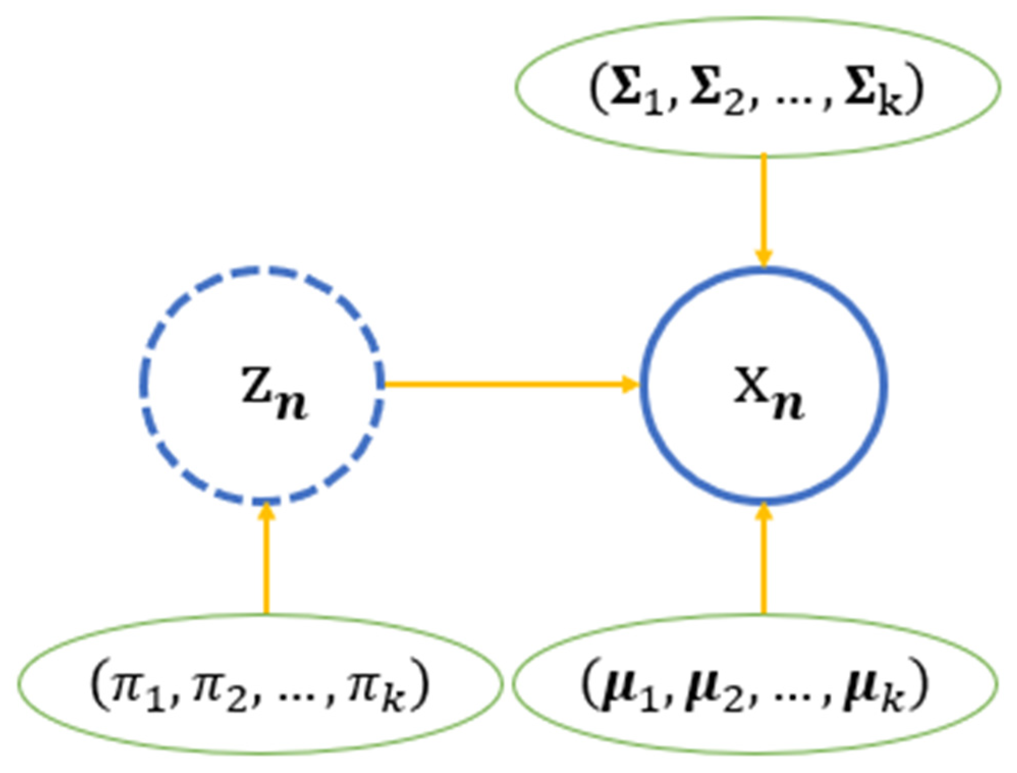
4.1. Gaussian Mixture Model

Building energy data are often a mixture of samples from different populations where the parameters differ from each other. A natural strategy is to identify these populations and generate new data points using respective populations where a Gaussian mixture model (GMM) is built. GMM is a simple linear superposition of Gaussian components, aimed at providing a richer class of density models than the single Gaussian [51]. GMM is also a generative model, wherein arbitrary amounts of data can be generated. While $K$-means, a special form of GMM, assigns an individual to the nearest center, GMM gives a soft allocation for all data points. GMM is an unsupervised method where a data point is assumed to belong to a component with a certain probability. A categorical latent variable $Z$ is adopted to determine a specific component by letting $Z_k=1$ and $Z_{-k}=0$, where $Z_{-k}$ is the elements other than $Z_k$. The marginal distribution of $Z$ is denoted as $P(Z_k=1)={\pi }_k$ with $\sum {\pi }_k=1$ for $k=1, 2,\dots ,K$. Thus, in Equation (1), the marginal distribution for the observable variable $\mathit{X}$ will be

$$p\left(\mathit{x}\right)={\displaystyle \sum }_{k=1}^K{\pi }_k\mathcal{N}\left(\mathit{x}|{\mathit{\mu }}_{\mathit{k}},{\mathsf{\Sigma }}_{\mathit{k}}\right),$$

(1)

where $\mathcal{N}\left(\mathit{x}|{\mathit{\mu }}_{\mathit{k}},{\mathsf{\Sigma }}_{\mathit{k}}\right)$ is the Gaussian density. A posterior probability for $Z_k$ when $\mathit{x}$ is given indicates how much each component contributes to the realization of $\mathit{x}$:

$$\gamma \left(k|х\right)=p\left(Z_k=1|\mathit{x}, \mathit{\mu }, \mathsf{\Sigma }\right)=\frac{{\pi }_k\mathcal{N}\left(\mathit{x}|{\mathit{\mu }}_{\mathit{k}},{\mathsf{\Sigma }}_{\mathit{k}}\right)}{{{\displaystyle \sum }}_{j=1}^K{\pi }_j\mathcal{N}\left(\mathit{x}|{\mathit{\mu }}_{\mathit{j}},{\mathsf{\Sigma }}_{\mathit{j}}\right)}$$

(2)

$\gamma \left(k|\mathsf{х}\right)$ in Equation (2) is also known as the responsibility probability allowing us to partition an observation into $K$ components. For a given set of independent observations ${\mathit{х}}_{\mathbf{1}}, {\mathit{х}}_{\mathbf{2}},\dots , {\mathit{х}}_{\mathit{N}}$ with sample size $N$, we assume that ${\mathsf{ᴢ}}_{\mathit{n}}$, $n=1, 2,\dots ,N$, is the latent variable for each observation. In addition to the location and shape parameters ${\mathit{\mu }}_{\mathit{k}}$ and ${\mathsf{\Sigma }}_{\mathit{k}}$, the marginal probabilities ${\pi }_1,{\pi }_2,\dots ,{\pi }_k$ also contribute the parameter space of the log-likelihood function in Equation (3):

$$ℒ\left(\mathit{\pi }, \mathit{\mu }, \mathsf{\Sigma }\right)=lnp\left(\mathit{x}|{\pi }_k,{\mathit{\mu }}_{\mathit{k}},{\mathsf{\Sigma }}_{\mathit{k}}\right)={\displaystyle \sum }_{n=1}^{N}ln\left[{\displaystyle \sum }_{k=1}^K{\pi }_k\mathcal{N}\left({\mathit{х}}_{\mathit{n}}|{\mathit{\mu }}_{\mathit{k}},{\mathsf{\Sigma }}_{\mathit{k}}\right)\right]$$

(3)

The graphical representation for an observation ${\mathit{х}}_{\mathit{n}}$ can be illustrated in Figure 1. The explicit form of the derivatives to Equation (3) is not available due to the summation term in the logarithm operation. The EM algorithm introduced in Section 4.2 and Section 4.3 will address this difficulty and evaluate its likelihood in a tractable way.

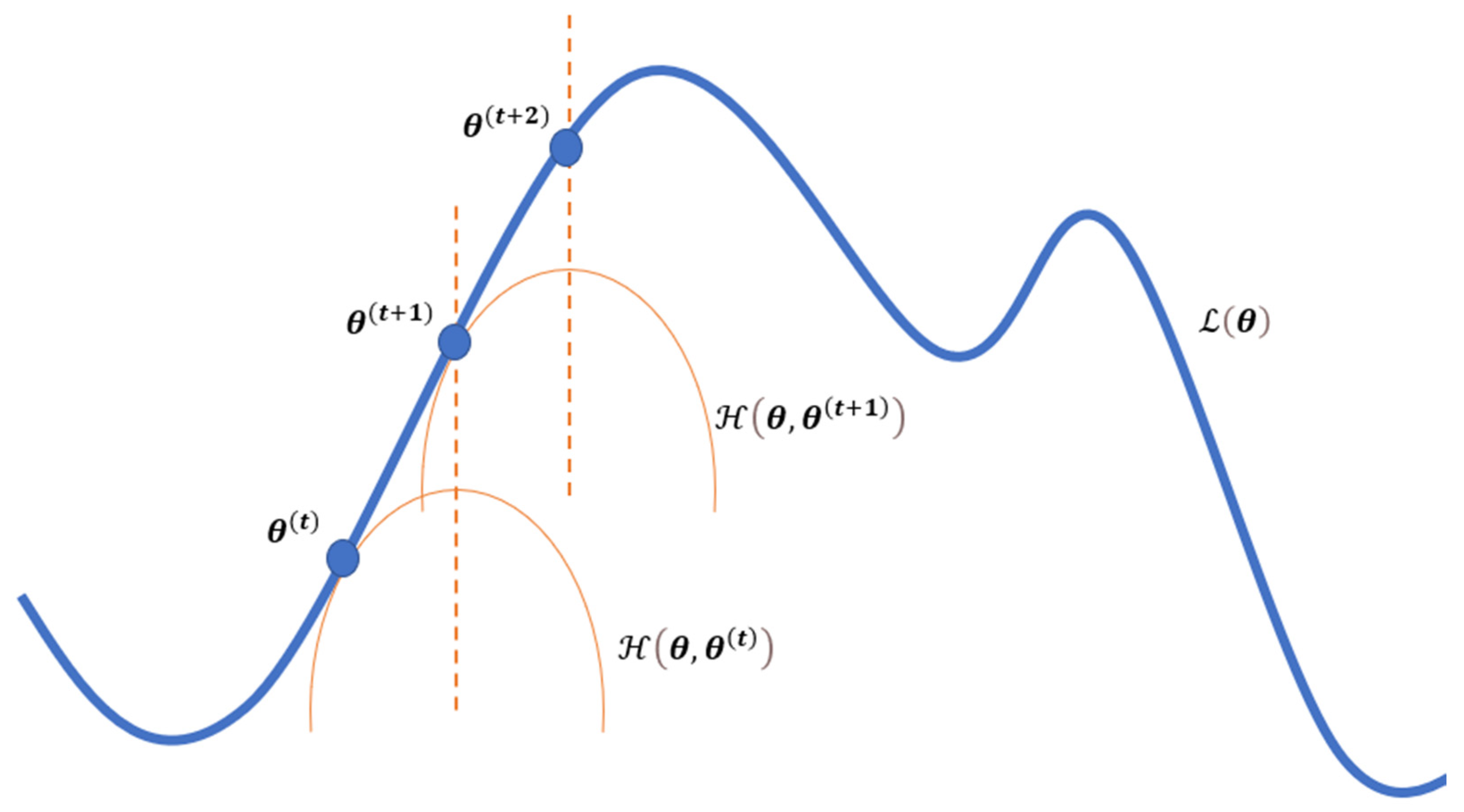
4.2. The Expectation-Maximization (EM) Algorithm

It has been proposed that an EM algorithm might be used to iteratively compute maximum-likelihood with incomplete information, where many applications such as filling in missing data, grouping and censoring, variance components, hyperparameter estimation, reweighted least-squares and factor analysis are explicitly addressed [52]. EM is considered one of the top ten algorithms in data mining and simplifies the maximization procedures for GMM [53]. Density estimation for GMM via EM can also handle high-dimensional data [54]. Thus, for a parametrized probability model $P(\mathrm{X}|\mathit{\theta })$, the joint distribution $P(\mathrm{X},\mathrm{Z}|\mathit{\theta })$ is introduced to rewrite the log-likelihood as

$$ℒ\left(\mathit{\theta }\right)=lnP\left(\mathrm{X}|\mathit{\theta }\right)=lnP\left(\mathrm{X},\mathrm{Z}|\mathit{\theta }\right)-lnP\left(\mathrm{Z}|\mathrm{X},\mathit{\theta }\right),$$

(4)

where $\mathrm{X}$ is the observable variable and $\mathrm{Z}$ is the hidden variable. It should be noted that $lnP\left(\mathrm{X}|\mathit{\theta }\right)$ is given in the form of a random variable. It will be equivalent to ${\displaystyle \sum }_{i=1}^{N}lnP({х}_i|\mathit{\theta })$ when the sample $x_1, x_2,\dots , x_N$ is obtained. We denote a density function of $\mathrm{Z}$ as $q\left(\mathrm{Z}\right)$ with $q\left(\mathrm{Z}\right)>0$. Since $q\left(\mathrm{Z}\right)$ is irrelevant to $\mathit{\theta }$, taking an expectation to $lnP\left(\mathrm{X}|\mathit{\theta }\right)$ with regard to the distribution of $\mathrm{Z}$ will not affect the value of $ℒ\left(\mathit{\theta }\right)$. On the other hand, taking the expectation to the right-hand side in Equation (4) results in

$$ℒ\left(\mathit{\theta }\right)={\displaystyle {{\displaystyle \int }}_{\mathrm{Z}}^{ }}q\left(\mathrm{Z}\right)ln\frac{P\left(\mathrm{X},\mathrm{Z}|\mathit{\theta }\right)}{q\left(\mathrm{Z}\right)}d\mathrm{Z}-{\displaystyle {{\displaystyle \int }}_{\mathrm{Z}}^{ }}q\left(\mathrm{Z}\right)ln\frac{P\left(\mathrm{Z}|\mathrm{X},\mathit{\theta }\right)}{q\left(\mathrm{Z}\right)}d\mathrm{Z}.$$

(5)

In Equation (5), $-{\displaystyle {{\displaystyle \int }}_{\mathrm{Z}}^{ }}q\left(\mathrm{Z}\right)ln\frac{P\left(\mathrm{Z}|\mathrm{X},\mathit{\theta }\right)}{q\left(\mathrm{Z}\right)}d\mathrm{Z}$, known as the Kullback–Leibler divergence and denoted as $KL\left(q\parallel P\right)$, is used to measure the distance between $q\left(\mathrm{Z}\right)$ and $P\left(\mathrm{Z}|\mathrm{X},\mathit{\theta }\right)$ [55]. $KL\left(q\parallel P\right)$ takes the value of 0 when $q\left(\mathrm{Z}\right)=P\left(\mathrm{Z}|\mathrm{X},\mathit{\theta }\right)$, otherwise it is greater than 0. If we denote ${\displaystyle {{\displaystyle \int }}_{\mathrm{Z}}^{ }}q\left(\mathrm{Z}\right)ln\frac{P\left(\mathrm{X},\mathrm{Z}|\mathit{\theta }\right)}{q\left(\mathrm{Z}\right)}d\mathrm{Z}$ as the evidence lower bound (ELBO), $ℒ\left(\mathit{\theta }\right)$ can be represented in Equation (6) as

$$ℒ\left(\mathit{\theta }\right)=ELBO+KL\left(q\parallel P\right).$$

(6)

For fixed $\mathit{\theta }$ and ${х}_1, {х}_2,\dots , {х}_N$, $ℒ\left(\mathit{\theta }\right)\ge ELBO$. $ℒ\left(\mathit{\theta }\right)$ takes the value of its lower bound ELBO only when $KL\left(q\parallel P\right)=0$. Thus, the task becomes to find the estimate of $\mathit{\theta }$ such that

$$\begin{array}{l} {\widehat{\mathit{\theta }}}^{\left(t+1\right)}=arg \underset{\mathit{\theta }}{\max }ELBO\\ =\arg \underset{\mathit{\theta }}{\max }{{\displaystyle \int }}_{\mathrm{Z}}P\left(\mathrm{Z}|\mathrm{X},{\mathit{\theta }}^{\left(\mathit{t}\right)}\right)[lnP\left(\mathrm{X},\mathrm{Z}|\mathit{\theta }\right)-lnP\left(\mathrm{Z}|\mathrm{X},{\mathit{\theta }}^{\left(\mathit{t}\right)}\right)]d\mathrm{Z}\\ =\arg \underset{\mathit{\theta }}{\max } {\mathbb{E}}_{P\left(\mathrm{Z}|\mathrm{X},{\mathit{\theta }}^{\left(\mathit{t}\right)}\right)}\left[lnP\left(\mathrm{X},\mathrm{Z}|\mathit{\theta }\right)\right].\end{array}$$

(7)

${\mathit{\theta }}^{\left(\mathit{t}\right)}$ is fixed for $P\left(\mathrm{Z}|\mathrm{X},{\mathit{\theta }}^{\left(\mathit{t}\right)}\right)$ that is one of the specific options for $q\left(\mathrm{Z}\right)$ in Equation (7). The superscript $\left(t\right)$ indicates the values obtained from the last iteration of the EM algorithm. Hence, ${\displaystyle {{\displaystyle \int }}_{\mathrm{Z}}^{ }}P\left(\mathrm{Z}|\mathrm{X},{\mathit{\theta }}^{\left(\mathit{t}\right)}\right)lnP\left(\mathrm{Z}|\mathrm{X},{\mathit{\theta }}^{\left(\mathit{t}\right)}\right)d\mathrm{Z}$ is independent of $\mathit{\theta }$ and can be treated as constant in the estimation. It should be noted that $P\left(\mathrm{Z}|\mathrm{X},\mathit{\theta }\right)$ is the ideal representation of the form of $q\left(\mathrm{Z}\right)$ in some specific models. For implicit $q\left(\mathrm{Z}\right)$ that is hard to obtain, an approximation method is usually applied to find the best $q\left(\mathrm{Z}\right)$.

Two recursive steps for updating ${\widehat{\mathit{\theta }}}^{\left(t+1\right)}$ in Equation (7) form the EM algorithm. In the E-step, we use old ${\mathit{\theta }}^{\left(\mathit{t}\right)}$ to find the posterior distribution for the latent variable, which is used to calculate the expectation of complete-data likelihood:

$$\mathscr{H}\left(\mathit{\theta };{\mathit{\theta }}^{\left(\mathit{t}\right)}\right)={\mathbb{E}}_{P\left(\mathrm{Z}|\mathrm{X},{\mathit{\theta }}^{\left(\mathit{t}\right)}\right)}\left[lnP\left(\mathrm{X},\mathrm{Z}|\mathit{\theta }\right)\right].$$

(8)

In the M-step, ${\mathit{\theta }}^{\left(\mathit{t}+\mathbf{1}\right)}$ is updated by maximizing Equation (8):

$${\widehat{\mathit{\theta }}}^{\left(t+1\right)}=arg \underset{\mathit{\theta }}{\max }\mathscr{H}\left(\mathit{\theta };{\mathit{\theta }}^{\left(\mathit{t}\right)}\right).$$

(9)

An iterative evaluation of Equations (8) and (9) guarantees the convergence of $ℒ\left(\mathit{\theta }\right)$ [56]. An illustration of this process can be seen in Figure 2. The M-step searches the new parameter to increase the value of $\mathscr{H}\left(\mathit{\theta }; •\right)$ that is further increased by plugging to $ℒ\left(\mathit{\theta }\right)$ because the property $ℒ\left(\mathit{\theta }\right)\ge ELBO$ always holds. The convergence will be found until $\mathit{\theta }$ does not significantly update its value or $ℒ\left(\mathit{\theta }\right)$ does not improve.

4.3. Parameter Estimation for GMM

$\mathscr{H}\left(\mathit{\theta }; {\mathit{\theta }}^{\left(\mathit{t}\right)}\right)$ is evaluated on the joint log-likelihood with complete data, which differs from the incomplete log-likelihood described in Equation (3). If we let the distribution of latent variable $Z$ be $P\left(Z\right)={\displaystyle \prod }_{k=1}^K{\pi }_k^{z_k}$ and the conditional distribution be $P\left(X|Z\right)={\displaystyle \prod }_{k=1}^K\mathcal{N}{\left(\mathit{x}|{\mathit{\mu }}_{\mathit{k}},{\mathsf{\Sigma }}_{\mathit{k}}\right)}^{z_k}$, the likelihood for complete data is a product of the two distributions:

$$P\left( {\mathit{х}}_{\mathit{n}}, z_{\mathit{n}}|\mathit{\pi }, \mathit{\mu }, \mathsf{\Sigma }\right)={\displaystyle \prod }_{n=1}^N{\displaystyle \prod }_{k=1}^K{\pi }_k^{z_{nk}}\mathcal{N}{\left( {\mathit{х}}_{\mathit{n}}|{\mathit{\mu }}_{\mathit{k}},{\mathsf{\Sigma }}_{\mathit{k}}\right)}^{z_{nk}},$$

(10)

where $z_{nk}$ indicates the $k^{th}$ component for ${\mathit{х}}_{\mathit{n}}$. Compared with Equation (3), the benefit for evaluating Equation (10) is that the logarithm part of $lnP\left( {\mathit{х}}_{\mathit{n}}, z_{\mathit{n}}|\mathit{\pi }, \mathit{\mu }, \mathsf{\Sigma }\right)$ will not be calculated on any summation terms, and there will only be a linear relationship between the latent variable $Z$ and the observed variable, namely

$$lnP\left( {\mathit{х}}_{\mathit{n}}, z_{\mathit{n}}|\mathit{\pi }, \mathit{\mu }, \mathsf{\Sigma }\right)={\displaystyle \sum }_{n=1}^N{\displaystyle \sum }_{k=1}^K{z}_{nk}\left[ln{\pi }_k+ln\mathcal{N}\left( {\mathit{х}}_{\mathit{n}}|{\mathit{\mu }}_{\mathit{k}},{\mathsf{\Sigma }}_{\mathit{k}}\right)\right].$$

(11)

Based on Equation (11), $\mathscr{H}\left(\mathit{\theta }, {\mathit{\theta }}^{\left(\mathit{t}\right)}\right)$ can be easily specified as

$$\begin{array}{l}\mathscr{H}\left(\mathit{\pi }, \mathit{\mu }, \mathsf{\Sigma }; {\mathit{\pi }}^{\left(\mathit{t}\right)}, {\mathit{\mu }}^{\left(\mathit{t}\right)}, {\mathsf{\Sigma }}^{\left(\mathit{t}\right)}\right)={\mathbb{E}}_{P\left(z_{\mathit{n}}| {\mathit{х}}_{\mathit{n}},{\mathit{\pi }}^{\left(\mathit{t}\right)}, {\mathit{\mu }}^{\left(\mathit{t}\right)}, {\mathsf{\Sigma }}^{\left(\mathit{t}\right)}\right)}\left[lnP\left( {\mathit{х}}_{\mathit{n}}, z_{\mathit{n}}|\mathit{\pi }, \mathit{\mu }, \mathsf{\Sigma }\right)\right]\\ ={\displaystyle {\displaystyle \sum }_{n=1}^N}{\displaystyle {\displaystyle \sum }_{k=1}^K}{\gamma }_{nk}\left[ln{\pi }_k+ln\mathcal{N}\left( {\mathit{х}}_{\mathit{n}}|{\mathit{\mu }}_{\mathit{k}},{\mathsf{\Sigma }}_{\mathit{k}}\right)\right],\end{array}$$

(12)

where ${\gamma }_{nk}=\mathbb{E}\left[z_{nk}\right]$ is the responsibility probability for a given ${\mathit{х}}_{\mathit{n}}$ to be partitioned into component $k$. Thus, the specification of $\gamma \left(k|х\right)$ in Equation (2), ${\gamma }_{nk}$, can be evaluated by

$${\gamma }_{nk}=\gamma \left(k|{\mathit{х}}_{\mathit{n}}\right)=\frac{{\pi }_k\mathcal{N}\left({\mathit{х}}_{\mathit{n}}|{\mathit{\mu }}_{\mathit{k}},{\mathsf{\Sigma }}_{\mathit{k}}\right)}{{{\displaystyle \sum }}_{j=1}^K{\pi }_j\mathcal{N}\left({\mathit{х}}_{\mathit{n}}|{\mathit{\mu }}_{\mathit{j}},{\mathsf{\Sigma }}_{\mathit{j}}\right)}.$$

(13)

The maximization of Equation (12) is in a tractable form if taking derivatives to the parameters. Due to the constraint ${\displaystyle \sum }{\pi }_k=1$, a Lagrange multiplier $\lambda$ is introduced for ${\pi }_k$. Finally, the E-step for GMM is to evaluate the log-likelihood given ${\mathit{\theta }}^{\left(\mathit{t}\right)}=\{{\mathit{\pi }}^{\left(\mathit{t}\right)}, {\mathit{\mu }}^{\left(\mathit{t}\right)}, {\mathsf{\Sigma }}^{\left(\mathit{t}\right)}\}$ and the M-step updates the parameters:

$$\begin{array}{l}{\mathit{\mu }}_{\mathit{k}}{}^{\left(\mathit{t}+\mathbf{1}\right)}=\frac{1}{{{\displaystyle \sum }}_{n=1}^N{\gamma }_{nk}}{\displaystyle {\displaystyle \sum }_{n=1}^N}{\gamma }_{nk}{\mathit{х}}_{\mathit{n}};\\ {\mathsf{\Sigma }}_{\mathit{k}}{}^{\left(\mathit{t}+\mathbf{1}\right)}=\frac{1}{{{\displaystyle \sum }}_{n=1}^N{\gamma }_{nk}}{\displaystyle {\displaystyle \sum }_{n=1}^N}{\gamma }_{nk}\left({\mathit{х}}_{\mathit{n}}-{\mathit{\mu }}_{\mathit{k}}{}^{\left(\mathit{t}+\mathbf{1}\right)}\right){({\mathit{х}}_{\mathit{n}}-{\mathit{\mu }}_{\mathit{k}}{}^{\left(\mathit{t}+\mathbf{1}\right)})}^T;\\ {\pi }_k{}^{\left(t+1\right)}=\frac{{{\displaystyle \sum }}_{n=1}^N{\gamma }_{nk}}{N}.\end{array}$$

When all the parameters are updated, we return to the E-step and evaluate Equation (13). The terminal of the algorithm, as introduced in Section 4.2, is reached either by observing stable $\mathit{\theta }$ or $ℒ\left(\mathit{\theta }\right)$.

5. Data and Performance

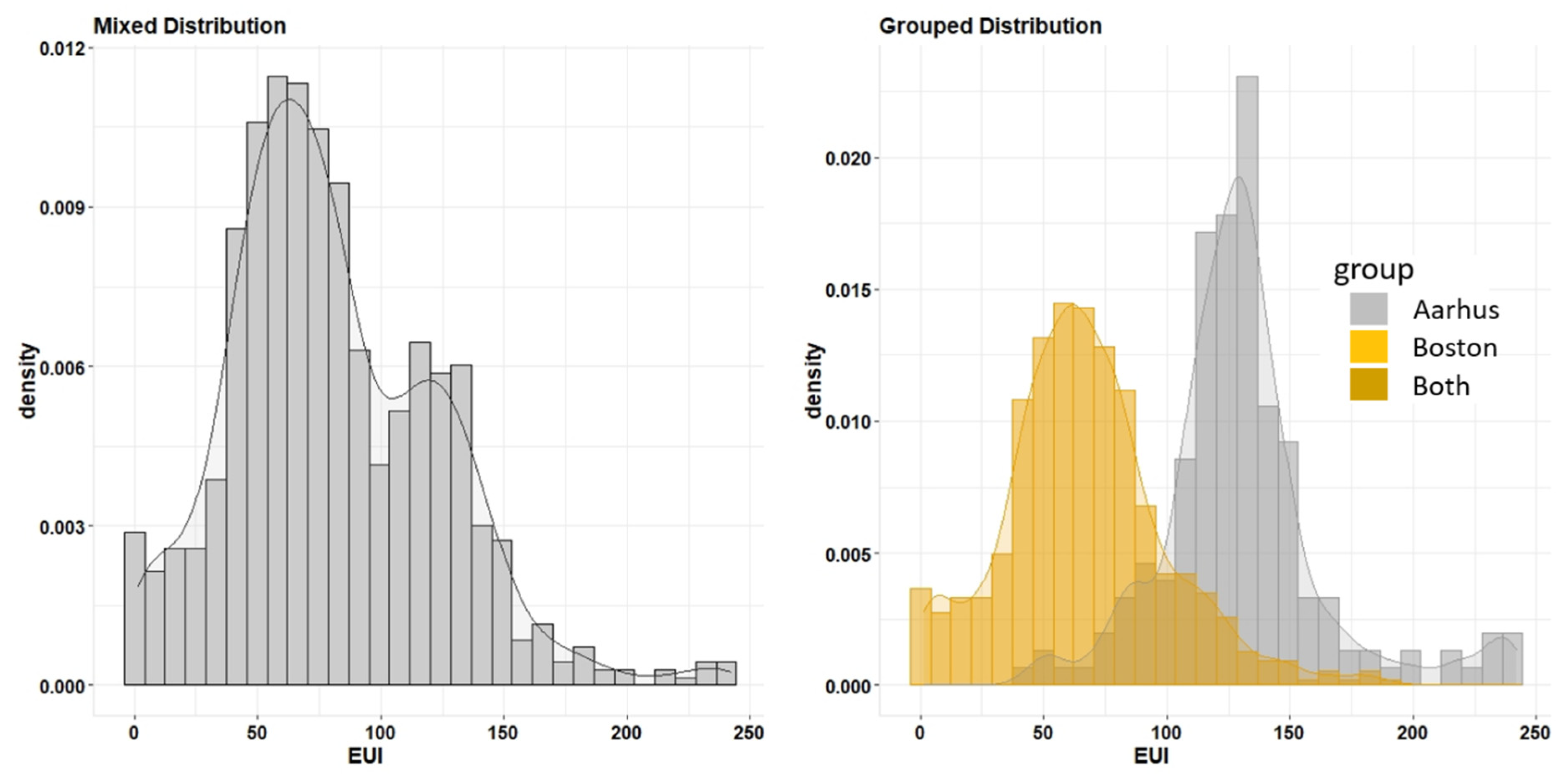
5.1. Test Datasets

This paper considers two different datasets to validate the proposed method. Both datasets are well organized and free to use. The first one is the public building energy and water use data from Boston in the United States (the data are available at https://data.boston.gov/dataset/building-energy-reporting-and-disclosure-ordinance). The dataset was collected according to the Building Energy Reporting and Disclosure Ordinance (BERDO), which allows different types of building stakeholders to track their energy usage and greenhouse gas emissions and provides an assessment source for local government to implement energy-saving policies. In the original file from 2019 there were 28 variables in total. This includes general variables related to categories such as building name, location, physical information and energy-related variables. The variable Energy Use Intensity (EUI) reflects total annual energy consumption divided by the gross floor area. EUI is an effective measurement of energy performance. By eliminating the missing values and outliers from the Boston dataset, we identified 659 buildings labeled as multifamily housing.

The second dataset was collected in Aarhus (Århus in Denish), Denmark in 2020 in order to examine the district heating (DH) efficiency of different Danish building types (the data are available at https://data.mendeley.com/datasets/v8mwvy7p6r/1) [57]. From this dataset we extracted the EUI data for multifamily housing built between the 1960s and the 1980s and identified 183 buildings. The mean values of EUIs for Boston and Aarhus were 66.68 and 130.46 respectively. Given the two samples now comprised homogeneous information, we merged them into one and assumed the number of populations to be two. Thus, univariate Gaussian distribution was considered.

In addition, our calculations took the variable age group from the Danish dataset, representing the period when the building was built, as a new population indicator to illustrate the bivariate case. The segmentation was determined by shifts in Danish building traditions and the tightening of energy requirements in Danish Building Regulations. Two specific age groups were chosen to constitute the populations: ‘1951–1960’ with 3461 buildings and ‘After 2015’ with 927. We then selected a secondary variable, Ga, to measure the daily heat load variation of these buildings since we postulated that the load variation may form a representative feature for both populations. Ga is calculated as the accumulated positive difference between the hourly and daily average heat loads during a year divided by both the annual average heat load and the number of hours (8760) in the year. Most of the values of Ga were around 0.2 indicating 20% load deviations on average. Thus, two populations (two age groups) and two variables (EUI and Ga) were constructed only from the Danish dataset for the bivariate case.

5.2. The Performance of EM Algorithm

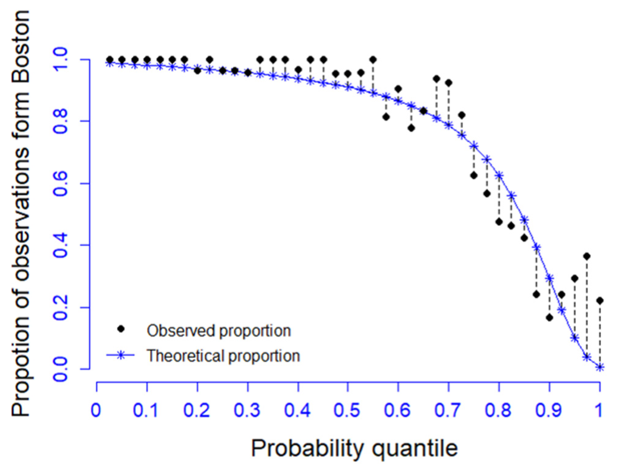
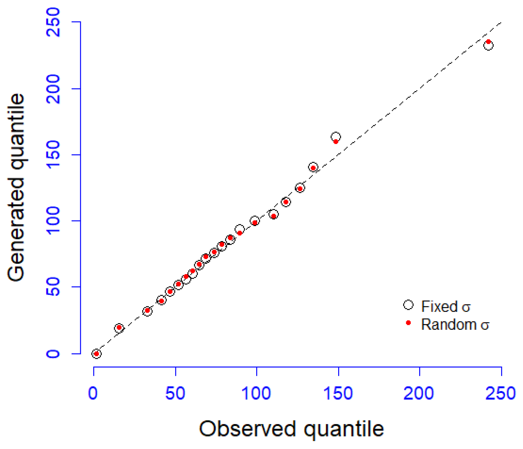
5.2.1. The Univariate Case

The histograms are plotted to present the mixed and grouped distribution of EUIs for both cities. In the left panel of Figure 3, the mixed distribution created two peaks, although there was no obvious separation in the overlapped part. The true distributions can, however, be seen quite clearly in the grouped (separated) distribution displayed in the right panel of Figure 3. One limitation when using a Gaussian distribution is that the value of EUI cannot be negative. A truncated Gaussian may be a more appropriate representation. However, since all the truncated data points belonged to the Boston population, using GMM will not affect the responsibility probability ${\gamma }_{nk}$ when conducting the E-step. Thus, we still follow the Gaussian assumption. If Gaussian property is severely violated, for example, because of the heat load variation in the bivariate variables, a Box-Cox transformation is required before implementing EM.

Another issue for the parameter estimation is to determine the initial values of $\mathit{\theta }$. It is not a difficult task to compare several combinations for the univariate case, but it will become a problem when the parameter size is large. Thus, we tested a number of possible combinations by varying the initial choice of ${\pi }_1, {\pi }_2, {\mu }_1, {\mu }_2, {\sigma }_1, {\sigma }_2$ and applied the same scheme to the bivariate case. More details on this process can be found in previous work on the setting of initial values [58]. The choice was determined by considering whether the final estimation could well represent both populations. The empirical results showed that the choices of ${\pi }_1, {\pi }_2, {\sigma }_1, {\sigma }_2$ did not seem to be dominant for the convergence, and we simply took ${\pi }_1={\pi }_2=0.5$ and ${\sigma }_1, {\sigma }_2$ to be the sample standard deviations. On the other hand, close values for ${\mu }_1$ and ${\mu }_2$ failed to separate the populations. In most of the experiments, ${\mu }_1$ and ${\mu }_2$ converged to a single value. Thus, we initialized ${\mu }_1$ and ${\mu }_2$ by letting them be constrained in the upper and lower 1/3 quantile of the mixed population, respectively. Further, one hundred initial values for ${\mu }_1$ and one hundred for ${\mu }_2$ were randomly generated to obtain ten thousand combinations in which we randomly opted ten for evaluating the performance.

The ten sets of parameters are summarized in

Table 1. Summary of the parameter estimation for fixed variance.

Population	Parameter	Min	Max	Mean	True Value	Error
Boston	${\mu }_1$	66.03	67.07	66.71	66.68	0.04%
	${\sigma }_1$	30.99	31.60	31.39	32.62	3.77%
	${\pi }_1$	0.76	0.78	0.77	0.78	1.28%
Aarhus	${\mu }_2$	126.84	129.23	128.33	130.46	1.63%
	${\sigma }_2$	39.33	39.48	39.38	34.00	15.8%
	${\pi }_2$	0.22	0.24	0.23	0.22	4.55%

. For every parameter, there was no significant variation, and the mean values can be used to represent ${\widehat{\mu }}_1$ and ${\widehat{\mu }}_2$. We also computed the absolute errors in percentage terms between the mean and true values. Most of them were within 5%, while the overestimation of ${\sigma }_2$ for Aarhus might be due to the slightly smaller estimation for ${\mu }_2$. Unlike fixed initial values, we also allowed for random variations up to 25% for ${\sigma }_1$ and ${\sigma }_2$ to validate our argument. As

Table 2. Summary of the parameter estimation for random variance.

Population	Parameter	Min	Max	Mean	True Value	Error
Boston	${\mu }_1$	66.00	67.42	66.59	66.68	0.13%
	${\sigma }_1$	30.98	31.80	31.32	32.62	3.98%
	${\pi }_1$	0.76	0.79	0.77	0.78	1.28%
Aarhus	${\mu }_2$	126.65	129.97	128.00	130.46	1.88%
	${\sigma }_2$	39.35	39.48	39.42	34.00	15.9%
	${\pi }_2$	0.21	0.24	0.23	0.22	4.55%

shows, the result resembled Table 1. The same conclusion could be drawn for ${\pi }_1$ and ${\pi }_2$, which are not shown here. It is also observed that the performance of the log-likelihood values in Figure 4 is uniform. All of the experiments stopped within 15 updates and seemed to converge at the same point. In other words, it is enough to make inferences based on current estimations.

We created two scenarios and assigned the sample points to the population with the larger density for classification. Two corresponding confusion matrices are presented in

Table 3. Classification accuracy for the univariate case.

Population (Predicted)	$\mathbf{True} \mathbf{Population}, \mathbf{Fixed} \sigma$		$\mathbf{True} \mathbf{Population}, \mathbf{Random} \sigma$
	Boston	Aarhus	Boston	Aarhus
Boston	72.92%	7.13%	73.40%	7.72%
Aarhus	5.34%	14.61%	4.87%	14.01%

. We divided all the data points into four categories: true Boston, false Boston, true Aarhus and false Aarhus. The accuracy is the sum of both true classifications that is close to 90%.

We then demonstrated the fitness between theoretical and empirical proportions. Proportion here refers to the quotient for which Boston’s EUI should theoretically and empirically account. Theoretical proportion is made by

$${\mathcal{P}}_{th}\left(Boston\right)=\frac{0.77\mathcal{N}\left(\tilde{\mathit{x}}|66.71, 31.39\right)}{0.77\mathcal{N}\left(\tilde{\mathit{x}}|66.71, 31.39\right)+0.23\mathcal{N}\left(\tilde{\mathit{x}}|128.33, 39.38\right)},$$

where $\tilde{\mathit{x}}$ corresponds to the probability quantile segmentation on the x-axis in Figure 5 for the mixed distribution. Similarly, the empirical proportion, ${\mathcal{P}}_{em}\left(Boston\right)$, counts the number of data points from Boston divided by all data points between two adjacent values of $\tilde{\mathit{x}}$. For example, if 100% of the observations are taken from Boston, ${\mathcal{P}}_{th}\left(Boston\right)$ should be extremely close to 1 at the quantile 0. Both ${\mathcal{P}}_{th}\left(Boston\right)$ and ${\mathcal{P}}_{em}\left(Boston\right)$ are supposed to decrease because ${\widehat{\mu }}_2$ is greater than ${\widehat{\mu }}_1$. Thus, the results showed a good fit except for the quantiles close to 1 on the bottom right corner. This is because of the long tail of Boston’s EUI. However, there were only a total of eight data points in this area, which is a minor deviation compared with ${\mathcal{P}}_{th}\left(Boston\right)$. The performance for Aarhus would look exactly the same just by vertically reversing Figure 5.

Given the results, we have drawn an additional two-step random sampling from the distributions to examine the generated EUIs. In step 1, we created a vector to store a random sequence of 0s and 1s that imply to which population a generated point belongs. The probabilities are taken as $P\left(I=0\right)=0.77$ and $P\left(I=1\right)=0.23$, where I is the indicator. The length of the vector is the same as the one of the observed sample, namely 842. In step 2, Gaussian random samples were drawn for each population to constitute the generated data. The quantile–quantile plot is shown for both fixed and random initial σs. As seen in Figure 6, the quantile values were taken every 5%. It is not surprising that neither setting for initial $\sigma$ differed a great deal, and almost all of the quantile values were located on the 45-degree line, which means that the quantile values matched each other. In this sense, the generated sample under GMM presented a reliable representation of the populations. Here we only used the true sample to validate a generated sample of the same size. When the method is used in an authentic context, the sample size will depend on the total number of buildings in the original cohort.

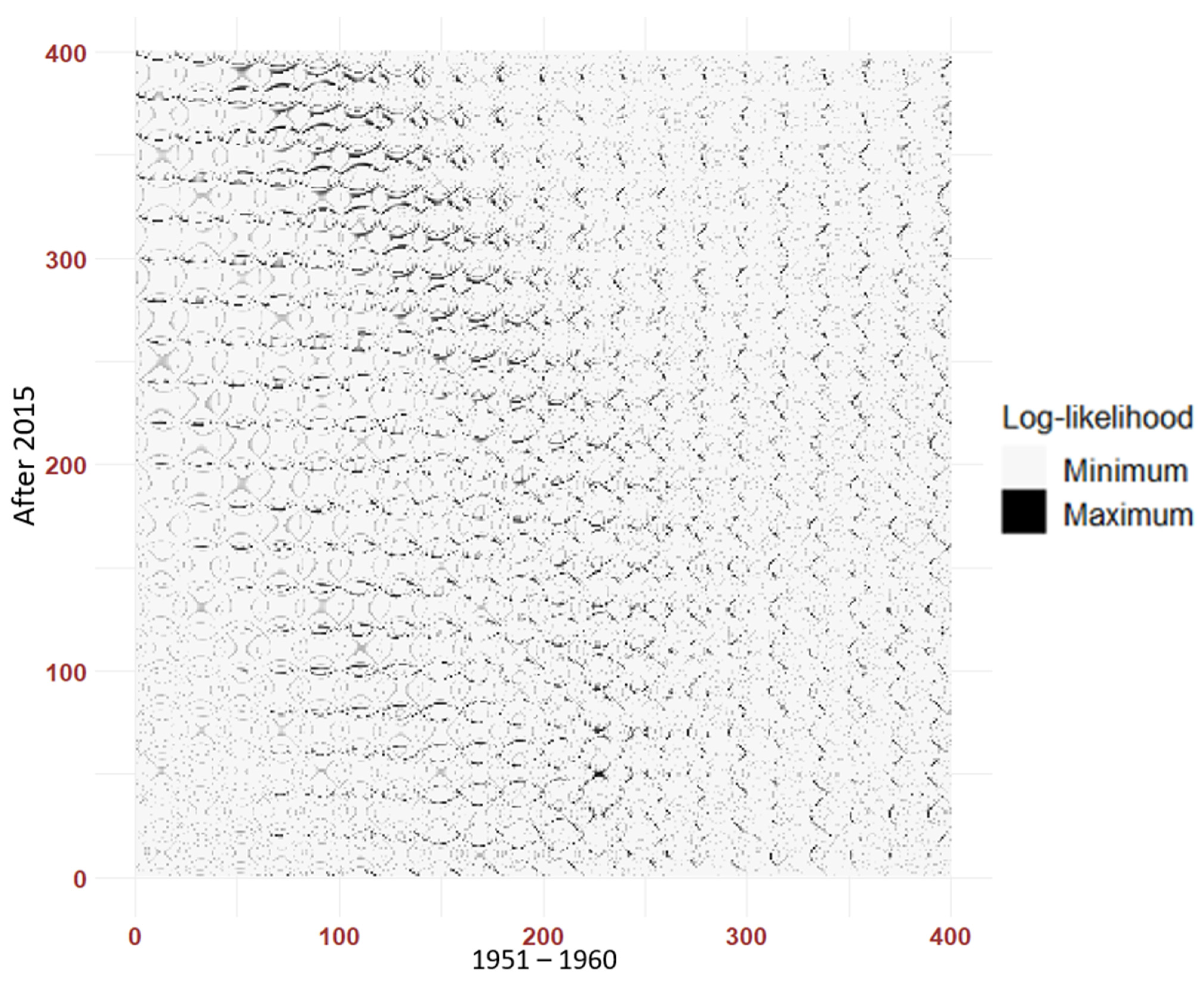
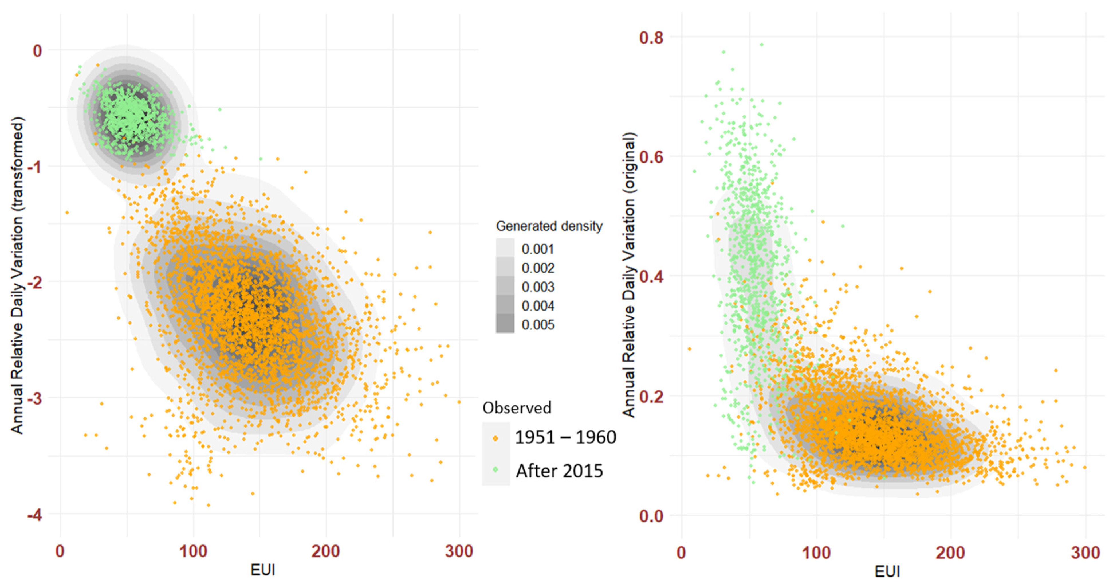
5.2.2. The Bivariate Case

Testing bivariate case requires more parameters to be estimated. The selection of the initial values followed the same paradigms that were adopted for the univariate case. In order to keep the Gaussian property, as mentioned in Section 5.2.1, the daily heat load variation (Ga) was treated by Box-Cox transformation [59]. Since the estimations then became complex, we also increased the number of experiments for determining the estimates. We picked 20 initial values from each of the population means: ${\mu }_{EUI1}$, ${\mu }_{Ga1}$, ${\mu }_{EUI2}$ and ${\mu }_{Ga2}$. The number of combinations became ${20}^4=\mathrm{160,000}$. In all the experiments, we highlighted the combinations with a log-likelihood in the top 10%. We present the resulting pattern in Figure 7 where 400 combinations were located on the x-axis for the population ‘1951–1960’, while 400 for the population ‘After 2015’ were located on the y-axis. The combinations were arranged from {minimum EUI, minimum Ga} to {minimum EUI, maximum Ga} and then to {maximum EUI, maximum Ga}. The figure shows that there were slight periodic patterns among the bigger $20\times 20$ grids. Higher log-likelihood was slightly denser in the top left part. In almost all the bigger $20\times 20$ grids, however, high log-likelihood could always be found. Thus, the selection of initial values for the EM algorithm in the bivariate case appears to be somewhat isotropic at finding estimates with high log-likelihood values.

Something similar happened when we summarized the results of the 10% experiments in

Table 4. Summary of the parameter estimation in the bivariate case.

Building Age Group	Parameter	Min	Max	Mean	True Value	Error
1951−1960	${\mu }_{EUI1}$	142.43	142.51	142.46	142.36	0.07%
	${\mu }_{Ga1}$(transformed)	−2.31	−2.31	−2.31	−2.31	0.00%
	${\sigma }_{EUI1}^2$	1706.44	1713.20	1710.78	1728.90	1.05%
	${\sigma }_{Ga1}^2$	0.26	0.26	0.26	0.26	0.00%
	$cov\left(EUI1,Ga1\right)$	−8.03	−7.81	−7.98	−8.17	2.33%
	${\pi }_{1951-1960}$	0.79	0.79	0.79	0.79	0.00%
After 2015	${\mu }_{EUI2}$	54.12	54.24	54.19	54.86	1.22%
	${\mu }_{Ga2}$(transformed)	−0.59	−0.59	−0.59	−0.59	0.00%
	${\sigma }_{EUI2}^2$	213.28	217.99	215.87	248.95	13.29%
	${\sigma }_{Ga2}^2$	0.02	0.02	0.02	0.02	0.00%
	$cov\left(EUI2,Ga2\right)$	−0.62	−0.58	−0.60	−0.67	10.45%
	${\pi }_{After 2015}$	0.21	0.21	0.21	0.21	0.00%

. In the bivariate case the overall errors decreased significantly compared with the univariate case. The majority were now below 3%. The reason for the bivariate model’s success might be that it is able to use more of the energy performance features to separate the populations more correctly. It should be noted that the estimated ${\widehat{\mu }}_{Ga}$ was not equal to the transformed mean value of Ga because the Box-Cox transformation is nonlinear. Thus, we only show the results for the transformed values here. We present both transformed and non-transformed Ga in the generative model evaluation later on. The classification accuracy is further computed in concordance with the univariate case in

Table 5. Classification accuracy for the bivariate case.

Age Group (Predicted)	True Population
	1951–1960	After 2015
1951–1960	78.56%	0.20%
After 2015	0.32%	20.92%

. Given the better parameter estimations, the true accuracy was over 99%.

The estimates obtained in Table 4 were used to generate density contours, with dense and sparse areas distinguished in the two-dimensional surface. We compared these with the true distributions because they disclose the real scales of the densities. The contours are displayed in the left panel of Figure 8, and show the comparison that is made for the transformed heat load variation, while the result of the non-transformed distributions is shown in the right panel. The generative models are supposed to characterize the distributions in both dense and sparse areas. Both panels had obvious and observable centers. Both of these centers converged at the densest part of the real data. In other words, the generative models represented the real data to an acceptable degree. As discussed in the univariate case, the actual number of generated samples depends on the city’s capacity to evaluate its energy performance with insufficient data.

6. Discussion

Using our proposed method to generate synthetic data is based on a distributional overview of the energy performance across all of the buildings in a district or urban area. However, our method does not take any spatial or temporal information into account. Imposing spatio-temporal mapping onto the synthetic data will help to draw an even better picture of building energy performance at the urban scale. As shown in Figure 9, spatial mapping takes the geolocations of buildings into consideration. Practically, the size of unlabeled data is far larger than labeled data. The performance of supervised learning models varies with limited labeled data. By including physical features, synthetic data are used to select and validate the supervised learning models for each population in a much more robust way.

The GMM method discussed in this work handles temporally aggregated data. With temporal mapping, it is possible to create higher time resolution data (for example hourly data) by including additional variables such as building class and hourly weather data. A set of buildings with known hourly energy consumption and building class could be taken as a set of reference buildings. By weighting from the reference buildings and sorting out a convex optimization problem, the synthetic data could then generate a set of energy performance profiles [60].

7. Conclusions

Big data are costly to collect and use. Even when this process is automated, many data collection systems operate with incomplete data or, in the case of building energy performance, are only able to collect data on a limited scale. From a statistical point of view, data from different groups are mixed together with little attempt made to distinguish between their representative populations. This hinders the efficient modeling of energy performance data, particularly at a large scale, and the construction of synthetic data for target groups.

In this paper, we proposed a GMM with an EM algorithm that can model building energy performance data for both univariate and bivariate cases. The energy performance indicators of a sample of buildings from Boston and Aarhus were adopted to segment mixed populations. For the univariate case, the Energy Use Intensity data from the two different cities were analyzed, and the updates were shown to have quick convergence. The derived models were able to capture the distributional features and to reflect the true population. The classification rate was almost 90%, and the generated data matched in quantile to the observed data. For the bivariate case, we showed that the inclusion of the new variable daily heat load variation further increased the power in parameter estimation, thus making the classification rate higher than in the univariate case. These data not only generate reliable density representations, but they also can be adjusted according to the real building capacity of a city with a spatio-temporal mapping.

Moreover, there are a number of topics in connection with these findings that would be interesting to explore in future studies.

• Firstly, in this paper we assumed that the number of populations was known. An interesting investigation would be to detect the optimal number of populations by introducing an objective function. Since Akaike information criterion (AIC) or Bayesian information criterion (BIC) reduces the effect on penalizing the model with small number of parameters, it is still an unsolved issue when the number of populations is small.
• Secondly, we suggest that other indicators of building energy use need to be considered because overall building performance is usually affected by multiple factors.
• Finally, it is also appealing that more probability distributions could be studied instead of using data transformation.

References

1. Cao, X.; Dai, X.; Liu, J. Building Energy-Consumption Status Worldwide and the State-of-the-Art Technologies for Zero-Energy Buildings during the Past Decade. Energy Build. 2016, 128, 198–213. [Google Scholar] [CrossRef]
2. Castillo-Calzadilla, T.; Macarulla, A.M.; Kamara-Esteban, O.; Borges, C.E. A Case Study Comparison between Photovoltaic and Fossil Generation Based on Direct Current Hybrid Microgrids to Power a Service Building. J. Clean. Prod. 2020, 244, 118870. [Google Scholar] [CrossRef]
3. D’Agostino, D.; Mazzarella, L. What Is a Nearly Zero Energy Building? Overview, Implementation and Comparison of Definitions. J. Build. Eng. 2019, 21, 200–212. [Google Scholar] [CrossRef]
4. Tabar, V.S.; Hagh, M.T.; Jirdehi, M.A. Achieving a Nearly Zero Energy Structure by a Novel Framework Including Energy Recovery and Conversion, Carbon Capture and Demand Response. Energy Build. 2021, 230, 110563. [Google Scholar] [CrossRef]
5. Hermelink, A.; Schimschar, S.; Boermans, T.; Pagliano, L.; Zangheri, P.; Armani, R.; Voss, K.; Musall, E. Towards Nearly Zero-Energy Buildings; European Commission: Köln, Germany, 2012. [Google Scholar]
6. Magrini, A.; Lentini, G.; Cuman, S.; Bodrato, A.; Marenco, L. From Nearly Zero Energy Buildings (NZEB) to Positive Energy Buildings (PEB): The next Challenge—The Most Recent European Trends with Some Notes on the Energy Analysis of a Forerunner PEB Example. Dev. Built Environ. 2020, 3, 100019. [Google Scholar] [CrossRef]
7. De Luca, G.; Ballarini, I.; Lorenzati, A.; Corrado, V. Renovation of a Social House into a NZEB: Use of Renewable Energy Sources and Economic Implications. Renew. Energy 2020, 159, 356–370. [Google Scholar] [CrossRef]
8. Kurnitski, J.; Saari, A.; Kalamees, T.; Vuolle, M.; Niemelä, J.; Tark, T. Cost Optimal and Nearly Zero (NZEB) Energy Performance Calculations for Residential Buildings with REHVA Definition for NZEB National Implementation. Energy Build. 2011, 43, 3279–3288. [Google Scholar] [CrossRef]
9. Li, W.; Zhou, Y.; Cetin, K.; Eom, J.; Wang, Y.; Chen, G.; Zhang, X. Modeling Urban Building Energy Use: A Review of Modeling Approaches and Procedures. Energy 2017, 141, 2445–2457. [Google Scholar] [CrossRef]
10. Pasichnyi, O.; Wallin, J.; Kordas, O. Data-Driven Building Archetypes for Urban Building Energy Modelling. Energy 2019, 181, 360–377. [Google Scholar] [CrossRef]
11. Ali, U.; Shamsi, M.H.; Bohacek, M.; Hoare, C.; Purcell, K.; Mangina, E.; O’Donnell, J. A Data-Driven Approach to Optimize Urban Scale Energy Retrofit Decisions for Residential Buildings. Appl. Energy 2020, 267, 114861. [Google Scholar] [CrossRef]
12. Fathi, S.; Srinivasan, R.; Fenner, A.; Fathi, S. Machine Learning Applications in Urban Building Energy Performance Forecasting: A Systematic Review. Renew. Sustain. Energy Rev. 2020, 133, 110287. [Google Scholar] [CrossRef]
13. Nutkiewicz, A.; Yang, Z.; Jain, R.K. Data-Driven Urban Energy Simulation (DUE-S): Integrating Machine Learning into an Urban Building Energy Simulation Workflow. Energy Procedia 2017, 142, 2114–2119. [Google Scholar] [CrossRef]
14. Hong, T.; Chen, Y.; Luo, X.; Luo, N.; Lee, S.H. Ten Questions on Urban Building Energy Modeling. Build. Environ. 2020, 168, 106508. [Google Scholar] [CrossRef] [Green Version]
15. Zhang, X.; Lovati, M.; Vigna, I.; Widén, J.; Han, M.; Gal, C.; Feng, T. A Review of Urban Energy Systems at Building Cluster Level Incorporating Renewable-Energy-Source (RES) Envelope Solutions. Appl. Energy 2018, 230, 1034–1056. [Google Scholar] [CrossRef]
16. Salim, F.D.; Dong, B.; Ouf, M.; Wang, Q.; Pigliautile, I.; Kang, X.; Hong, T.; Wu, W.; Liu, Y.; Rumi, S.K.; et al. Modelling Urban-Scale Occupant Behaviour, Mobility, and Energy in Buildings: A Survey. Build. Environ. 2020, 183, 106964. [Google Scholar] [CrossRef]
17. Perera, A.T.D.; Nik, V.M.; Chen, D.; Scartezzini, J.-L.; Hong, T. Quantifying the Impacts of Climate Change and Extreme Climate Events on Energy Systems. Nat. Energy 2020, 5, 150–159. [Google Scholar] [CrossRef] [Green Version]
18. Yang, Z.; Roth, J.; Jain, R.K. DUE-B: Data-Driven Urban Energy Benchmarking of Buildings Using Recursive Partitioning and Stochastic Frontier Analysis. Energy Build. 2018, 163, 58–69. [Google Scholar] [CrossRef]
19. Ma, J.; Cheng, J.C.P. Estimation of the Building Energy Use Intensity in the Urban Scale by Integrating GIS and Big Data Technology. Appl. Energy 2016, 183, 182–192. [Google Scholar] [CrossRef]
20. Risch, S.; Remmen, P.; Müller, D. Influence of Data Acquisition on the Bayesian Calibration of Urban Building Energy Models. Energy Build. 2021, 230, 110512. [Google Scholar] [CrossRef]
21. Goy, S.; Maréchal, F.; Finn, D. Data for Urban Scale Building Energy Modelling: Assessing Impacts and Overcoming Availability Challenges. Energies 2020, 13, 4244. [Google Scholar] [CrossRef]
22. Goodfellow, I.; Bengio, Y.; Courville, A. Deep Learning; Adaptive Computation and Machine Learning; MIT Press Ltd: Cambridge, MA, USA, 2016; ISBN 978-0-262-03561-3. [Google Scholar]
23. Chen, C.L.P.; Zhang, C. Data-Intensive Applications, Challenges, Techniques and Technologies: A Survey on Big Data. Inf. Sci. 2014, 275, 314–347. [Google Scholar] [CrossRef]
24. Ma, J.; Cheng, J.C.P.; Jiang, F.; Chen, W.; Wang, M.; Zhai, C. A Bi-Directional Missing Data Imputation Scheme Based on LSTM and Transfer Learning for Building Energy Data. Energy Build. 2020, 216, 109941. [Google Scholar] [CrossRef]
25. Marta, M.; Belinda, L. Simplified Model to Determine the Energy Demand of Existing Buildings. Case Study of Social Housing in Zaragoza, Spain. Energy Build. 2017, 149, 483–493. [Google Scholar] [CrossRef]
26. Cho, K.; Kim, S. Energy Performance Assessment According to Data Acquisition Levels of Existing Buildings. Energies 2019, 12, 1149. [Google Scholar] [CrossRef] [Green Version]
27. Guerra-Santin, O.; Tweed, C.A. In-Use Monitoring of Buildings: An Overview of Data Collection Methods. Energy Build. 2015, 93, 189–207. [Google Scholar] [CrossRef]
28. Laroca, R.; Barroso, V.; Diniz, M.A.; Goncalves, G.R.; Schwartz, W.R.; Menotti, D. Convolutional Neural Networks for Automatic Meter Reading. J. Electron. Imaging 2019, 28, 013023. [Google Scholar] [CrossRef]
29. Oti, A.H.; Kurul, E.; Cheung, F.; Tah, J.H.M. A Framework for the Utilization of Building Management System Data in Building Information Models for Building Design and Operation. Autom. Constr. 2016, 72, 195–210. [Google Scholar] [CrossRef] [Green Version]
30. Afroz, Z.; Burak Gunay, H.; O’Brien, W. A Review of Data Collection and Analysis Requirements for Certified Green Buildings. Energy Build. 2020, 226, 110367. [Google Scholar] [CrossRef]
31. Despotovic, M.; Koch, D.; Leiber, S.; Döller, M.; Sakeena, M.; Zeppelzauer, M. Prediction and Analysis of Heating Energy Demand for Detached Houses by Computer Vision. Energy Build. 2019, 193, 29–35. [Google Scholar] [CrossRef]
32. Wei, S.; Tien, P.W.; Calautit, J.K.; Wu, Y.; Boukhanouf, R. Vision-Based Detection and Prediction of Equipment Heat Gains in Commercial Office Buildings Using a Deep Learning Method. Appl. Energy 2020, 277, 115506. [Google Scholar] [CrossRef]
33. Gao, Y.; Ruan, Y.; Fang, C.; Yin, S. Deep Learning and Transfer Learning Models of Energy Consumption Forecasting for a Building with Poor Information Data. Energy Build. 2020, 223, 110156. [Google Scholar] [CrossRef]
34. Ryu, S.; Noh, J.; Kim, H. Deep Neural Network Based Demand Side Short Term Load Forecasting. Energies 2017, 10, 3. [Google Scholar] [CrossRef]
35. Lu, J.; Qian, J.; Zhang, Q.; Liu, S.; Xie, F.; Xu, H. Best Practices in China Southern Power Grid Competition of AI Short-Term Load Forecasting. In Proceedings of the 2020 12th IEEE PES Asia-Pacific Power and Energy Engineering Conference (APPEEC), Nanjing, China, 20–23 September 2020; pp. 1–5. [Google Scholar]
36. Wang, Y.; Liu, M.; Bao, Z.; Zhang, S. Short-Term Load Forecasting with Multi-Source Data Using Gated Recurrent Unit Neural Networks. Energies 2018, 11, 1138. [Google Scholar] [CrossRef] [Green Version]
37. Zhang, Y.; Ai, Q.; Li, Z.; Yin, S.; Huang, K.; Yousif, M.; Lu, T. Data Augmentation Strategy for Small Sample Short-term Load Forecasting of Distribution Transformer. Int. Trans. Electr. Energ. Syst. 2020, 30, 1–18. [Google Scholar] [CrossRef]
38. Acharya, S.K.; Wi, Y.; Lee, J. Short-Term Load Forecasting for a Single Household Based on Convolution Neural Networks Using Data Augmentation. Energies 2019, 12, 3560. [Google Scholar] [CrossRef] [Green Version]
39. Lai, C.S.; Mo, Z.; Wang, T.; Yuan, H.; Ng, W.W.Y.; Lai, L.L. Load Forecasting Based on Deep Neural Network and Historical Data Augmentation. IET Gener. Transm. Distrib. 2020. [Google Scholar] [CrossRef]
40. Goodfellow, I.J.; Pouget-Abadie, J.; Mirza, M.; Xu, B.; Warde-Farley, D.; Ozair, S.; Courville, A.; Bengio, Y. Generative Adversarial Nets. In Proceedings of the Advances in Neural Information Processing Systems 27 (NIPS), Montreal, QC, Canada, 8–13 December 2014. [Google Scholar]
41. Gui, J.; Sun, Z.; Wen, Y.; Tao, D.; Ye, J. A Review on Generative Adversarial Networks: Algorithms, Theory, and Applications. arXiv 2020, arXiv:2001.06937. [Google Scholar]
42. Wang, Z.; Hong, T. Generating Realistic Building Electrical Load Profiles through the Generative Adversarial Network (GAN). Energy Build. 2020, 224, 110299. [Google Scholar] [CrossRef]
43. Fekri, M.N.; Ghosh, A.M.; Grolinger, K. Generating Energy Data for Machine Learning with Recurrent Generative Adversarial Networks. Energies 2019, 13, 130. [Google Scholar] [CrossRef] [Green Version]
44. Gong, X.; Tang, B.; Zhu, R.; Liao, W.; Song, L. Data Augmentation for Electricity Theft Detection Using Conditional Variational Auto-Encoder. Energies 2020, 13, 4291. [Google Scholar] [CrossRef]
45. Hong, T.; Chou, S.K.; Bong, T.Y. Building Simulation: An Overview of Developments and Information Sources. Building Environ. 2000, 35, 347–361. [Google Scholar] [CrossRef]
46. Maile, T.; Bazjanac, V.; Fischer, M. A Method to Compare Simulated and Measured Data to Assess Building Energy Performance. Building Environ. 2012, 56, 241–251. [Google Scholar] [CrossRef]
47. Abuimara, T.; O’Brien, W.; Gunay, B.; Carrizo, J.S. Towards Occupant-Centric Simulation-Aided Building Design: A Case Study. Build. Res. Inf. 2019, 47, 866–882. [Google Scholar] [CrossRef]
48. Schiefelbein, J.; Rudnick, J.; Scholl, A.; Remmen, P.; Fuchs, M.; Müller, D. Automated Urban Energy System Modeling and Thermal Building Simulation Based on OpenStreetMap Data Sets. Building Environ. 2019, 149, 630–639. [Google Scholar] [CrossRef]
49. Hong, T.; Langevin, J.; Sun, K. Building Simulation: Ten Challenges. Build. Simul. 2018, 11, 871–898. [Google Scholar] [CrossRef] [Green Version]
50. Solmaz, A.S. A Critical Review on Building Performance Simulation Tools. Int. J. Sustain. Trop. Des. Res. Pract. UPM 2019, 12, 7–20. [Google Scholar]
51. Bishop, C.M. Pattern Recognition and Machine Learning; Springer Science+Business Media, LLC: New York, NY, USA, 2006. [Google Scholar]
52. Dempster, A.P.; Laird, N.M.; Rubin, D.B. Maximum Likelihood from Incomplete Data via the EM Algorithm. J. R. Stat. Soc. Ser. B (Methodol.) 1977, 39, 1–38. [Google Scholar]
53. Wu, X.; Kumar, V.; Quinlan, J.R.; Ghosh, J.; Yang, Q.; Motoda, H.; McLachlan, G.J.; Ng, A.; Liu, B.; Yu, P.S.; et al. Top 10 Algorithms in Data Mining. Knowl. Inf. Syst. 2008, 14, 1–37. [Google Scholar] [CrossRef] [Green Version]
54. Ghahramani, Z.; Jordan, M.I. Supervised Learning from Incomplete Data via an EM Approach; Morgan Kaufmann: San Francisco, CA, USA, 1994. [Google Scholar]
55. Kullback, S.; Leibler, R.A. On Information and Sufficiency. Ann. Math. Stat. 1951, 22, 79–96. [Google Scholar] [CrossRef]
56. Wu, C.F.J. On the Convergence Properties of the EM Algorithm. Ann. Stat. 1983, 11, 95–103. [Google Scholar] [CrossRef]
57. Kristensen, M.H.; Petersen, S. District Heating Energy Efficiency of Danish Building Typologies. Energy Build. 2021, 231, 110602. [Google Scholar] [CrossRef]
58. Blömer, J.; Bujna, K. Simple Methods for Initializing the EM Algorithm for Gaussian Mixture Models. arXiv 2013, arXiv:1312.5946v3. [Google Scholar]
59. Box, G.E.P.; Cox, D.R. An Analysis of Transformations. J. R. Stat. Soc. Ser. B (Methodol.) 1964, 26, 211–252. [Google Scholar] [CrossRef]
60. Roth, J.; Martin, A.; Miller, C.; Jain, R.K. SynCity: Using Open Data to Create a Synthetic City of Hourly Building Energy Estimates by Integrating Data-Driven and Physics-Based Methods. Appl. Energy 2020, 280, 115981. [Google Scholar] [CrossRef]
Figure 1. Graphical representation of a set of data points.
Buildings 11 00030 g001
Figure 2. Parameter update in the EM algorithm.
Buildings 11 00030 g002
Figure 3. Mixed and grouped distribution of EUI.
Buildings 11 00030 g003
Figure 4. Log-likelihood performance for the univariate case.
Buildings 11 00030 g004
Figure 5. Theoretical and empirical proportions.
Buildings 11 00030 g005
Figure 6. Quantile–quantile plot for observed and generated data.
Buildings 11 00030 g006
Figure 7. Distribution of top 10% log-likelihood for the combination of the initial values.
Buildings 11 00030 g007
Figure 8. Density comparisons for the bivariate generative model.
Buildings 11 00030 g008
Figure 9. Spatio-temporal mapping of urban buildings from GMM synthetic data.
Buildings 11 00030 g009