Dynamic Assessment of Axial Load in Tie-Rods by Means of Acoustic Measurements

Abstract

Tie-rods are structural elements of crucial importance in ancient buildings to ensure structural integrity and safety, so the assessment of their effectiveness via an estimation of the axial load is of great importance. Dynamic techniques are often employed using accelerometers to measure the frequency response of the tie-rods. In this work, the frequency response of tie-rods is obtained with acoustic recording, thus introducing general-purpose microphones to potentially replace more expensive and complex sensors in this application. Two microphones were tested, one of known technical characteristics, and a second for which they were unknown. A procedure was designed to overcome the technical limitations of the latter, and two experimental campaigns were conducted to test the proposed method.

1. Introduction

Tie-rods are slender metal beams mainly employed to absorb the horizontal thrust of arches and vaults, and to connect opposing walls of masonry structures in order to enhance their box-like behaviour. The use of modern metallic tie-rods dates back at least to the XV century [1], and their basic form hasn’t changed much since. They represent a fundamental element for the preservation of many Cultural Heritage (CH) assets (Figure 1).

Tie-rods have to be tensioned when installed. In the past this was achieved by heating up the rod before anchoring it to the walls [2]; nowadays, the load is usually applied via a nut with a torque wrench.

Evaluating the axial load of a tie-rod is a matter of some importance for the overall safety of the building: an inexistent or exaggerate load could suggest that the rod is damaged or inadequate, and may have to be replaced. A load value that clearly stands out in an otherwise similar series of tie-rod (such as those in galleries or courtyards) may be the symptom of some form of structural anomaly. The tensile load estimate may be particularly significant if associated with visible cracks on vaulted elements. It should be however noted that the evaluation of structural damage remains case-related and is always the subject of expert judgement. Nevertheless, it isn’t usually possible to fully evaluate the global structural safety, especially for CH assets, based on the value of a single parameter such as tie-rod axial load. Still, its knowledge constitutes an important step towards a more thorough comprehension of the building’s behaviour.

Several indirect methods to estimate a tie-rod’s axial load are described in the literature. They can be grouped in static and dynamic ones, based on the nature of their underlying mechanical relationships and of the consequent measurements that are being used. Static methods require the measurement of tie-rod deformation under a static force to estimate its pre-existent axial load. Several have been proposed, such as those in [3,4,5]. From an operational point of view, the main disadvantages in using a static method are: the need to hang a non-negligible weight to the tie-rod, the difficulties in measuring small deformations or displacements with the necessary accuracy [6], and in general the time and room required for the measurement.

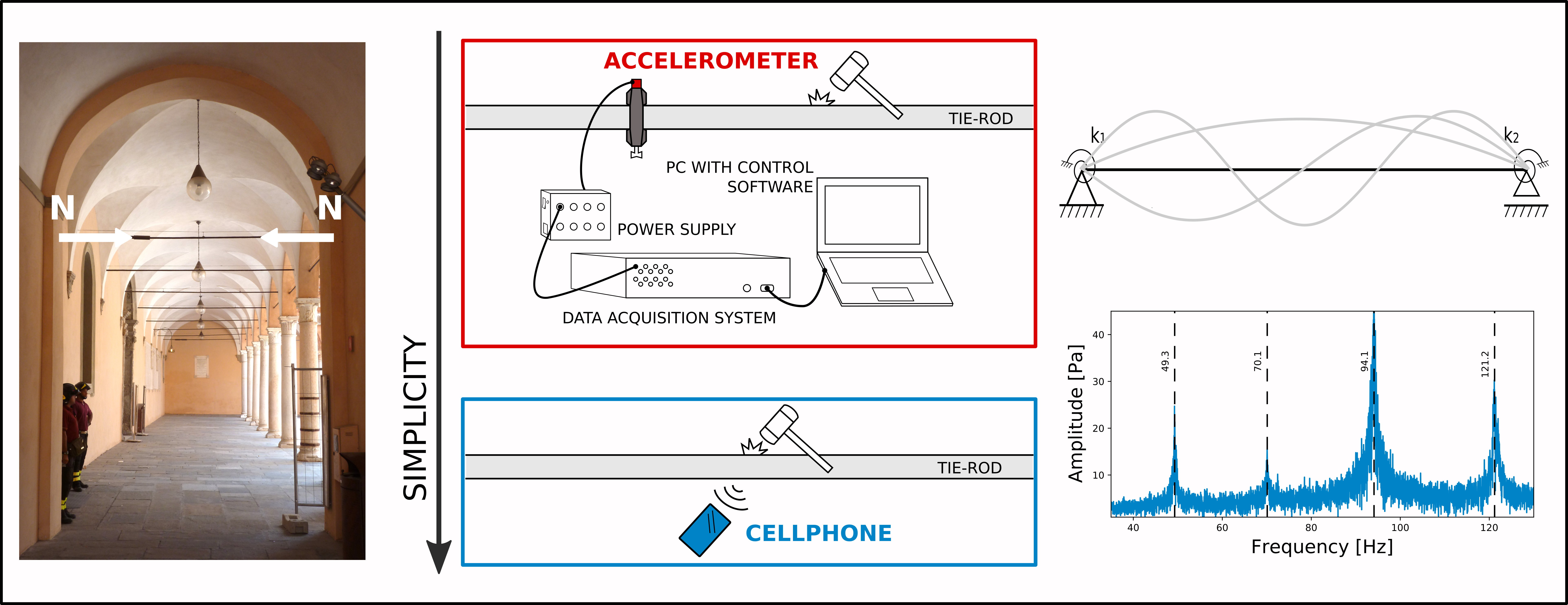
Dynamic methods, on the other hand, require the identification of vibrational characteristics of the rod, either natural frequencies alone or the former together with the corresponding modal shapes. Varying in complexity and accuracy, several dynamic methods have been proposed, such as those by [7,8,9,10]. Accelerometers are the sensors commonly used to identify tie-rod natural frequencies. To this purpose a dedicated data acquisition system, cables, and external power are needed. The consequent requirements in terms of time and money, together with the need for a professional operator, are the main downfalls of dynamic methods.

This paper is addressed to researchers and professionals in the CH preservation field. Here, we suggest the use of a portable, general purpose microphone to measure tie-rod natural frequencies in place of accelerometers. This enables quick, cheap and simple non-destructive dynamic evaluations, overcoming the aforementioned disadvantages.

Two distinct setups are proposed: one using a professional microphone sharing the same data acquisition system required for accelerometers, and a second using only a sensor embedded within a smartphone, which technical characteristics are unknown.

In the latter case, some of the natural frequencies of the measured tie-rod may fall outside the sensor’s range, so that there is a risk of ignoring an unknown number of natural frequencies during measurement. Since this poses a problem with all existing dynamic load-evaluation methods, a simple solution is proposed.

In the following section, more details are given concerning existing techniques to measure tie-rod natural frequencies, and the proposed one is detailed, highlighting its peculiarities. To compare the results of experimental campaigns performed using accelerometer and acoustic sensors, the estimation of the tensile load of the tested tie-rods is needed. This was done using a method well known and documented in the literature [7,8], which is also briefly presented in the next section to help better underst and the process.

In order to compare the two kinds of sensors, two testing campaigns in Certosa di Pisa and Palazzo Arcivescovile in Pisa (Italy) are detailed. The axial load of different tie-rods was evaluated using the aforementioned method and frequency measurements from both microphones and accelerometers. The following sections present and discuss the results, together with reflections over possible developments.

2. Materials and Methods

2.1. Axial Load Estimation Procedure

The present paper focuses on applying acoustic-based frequency identification as a necessary step towards the identification of tie-rod axial load. In this regard, a brief explanation of the chosen load estimation method is given here. The procedure is based on the ones proposed in [7,8], and it focuses on a comparison between a set of measured natural frequencies and a set of theoretical ones, generated from an analytical model.

The tie-rod is idealized as a Euler-Bernoulli beam [11] with elastic rotational restraints of given stiffness (see Figure 2). This allows to take into account the tie-rod’s bending stiffness, as well as the form and conditions of its anchorages to the wall.

Its free vibrations are modelled by a fourth grade differential Equation [11]:

$$EJ{v}^{IV}(x,t)-N{v}^{II}(x,t)+\rho A\ddot{v}(x,t)=0,$$

(1)

where $v(x,t)$ is the transverse displacement of a point on the tie-rod’s axis at time t, E is Young’s modulus, $\rho$ the material density, A and J respectively the cross section’s surface and its second moment, and finally N is the axial load. A general solution to the equation can be found by hypothesizing its separability [11], that is, by considering:

$$v(x,t)=y\left(x\right)·\tau \left(t\right).$$

(2)

This way, $\omega =\sqrt{-\frac{\ddot{\tau \left(t\right)}}{\tau \left(t\right)}}$ being the angular frequency of vibration of the tie-rod, we can consider the much simpler ODE:

$$y^{IV}\left(x\right)-\frac{N}{EJ}{y}^{II}\left(x\right)-\frac{\rho A}{EJ}{\omega }^{2}y\left(x\right)=0.$$

(3)

Its solution can be written, in real form, as [12]:

$$\begin{array}{c}\hfill y\left(x\right)=C_{1}cos\left(\lambda x\right)+C_{2}sin\left(\lambda x\right)+\\ \hfill +C_{3}cosh\left(\mu x\right)+C_{4}sinh\left(\mu x\right),\end{array}$$

(4)

where the following non-dimensional parameters have been used:

$$\begin{array}{c}\alpha =\frac{N{L}^2}{2EJ};\end{array}$$

(5)

$$\begin{array}{c}{\beta }_i={\omega }_i{L}^2\sqrt{\frac{\rho A}{EJ}};\end{array}$$

(6)

$$\begin{array}{c}2\lambda =\sqrt{-\alpha +\sqrt{{\alpha }^2+{\beta }^2}};\end{array}$$

(7)

$$\begin{array}{c}2\mu =\sqrt{\alpha +\sqrt{{\alpha }^2+{\beta }^2}}.\end{array}$$

(8)

Equation (4) can be used to write the relevant boundary conditions, obtaining a homogeneous linear system in the four unknowns $C_1$,...,$C_4$. The determinant of the associated matrix is then computed. The condition that the determinant is zero, necessary to exclude the null solution, is the desired function, tying together the tie-rod’s axial load, end restraints, geometrical and mechanical properties and, most important, natural frequencies. For it, an infinite number of solutions can be found, one for each natural frequency of the tie-rod. At this point, a numerical approach can be adopted. The experimental natural frequencies of the tie-rod $f_{exp}$ are given as inputs to an optimization algorithm. During the present research, the optimization was carried out with a combination of the Basinhopping algorithm (for global search) and Nelder-Mead method (for local minima), both already implemented in Python’s scipy library. The corresponding code is provided as Supplementary Material. 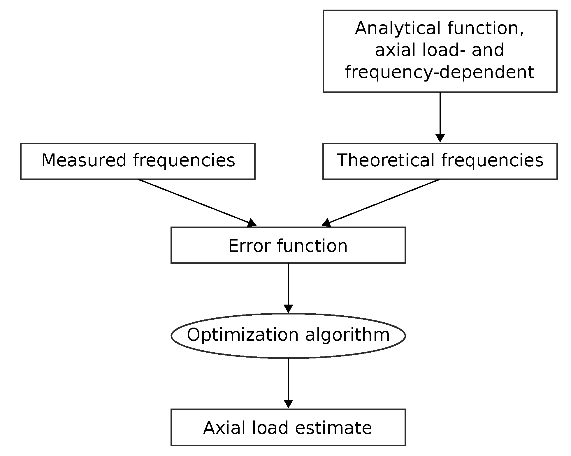Starting with a first estimate of the axial load, the algorithm derives a series of theoretical frequencies $f_{th}$ for an ideal tie-rod with such a load from the aforementioned function and evaluates an appropriate error function:

$$error=\sum _i\frac{f_{exp,i}-f_{th,i}}{f_{th,i}},$$

(9)

that is, the sum of the relative differences between the experimental ($f_{exp}$) and theoretical ($f_{th}$) frequencies for each mode i. The corresponding objective function is the one with zero error. The algorithm tries to minimize the objective function by evaluating the error function corresponding to other possible axial load values, in order to identify the one that produces frequencies the most similar to the measured ones. Figure 3 shows a flow diagram summarizing the adopted method.

2.2. Existing Techniques to Measure Tie-Rod Natural Frequencies

The identification of tie-rod natural frequencies can be carried out using any instrument capable of measuring the motion characteristics (displacement, velocity, acceleration) of the rod’s axis. As of today, the most used devices are accelerometers [6,7,8,9,10,13,14,15,16,17]. These sensors may be used to perform either an Operational Modal Analysis (OMA) [16,17] or an Experimental Modal Analysis (EMA) [6,7,8,9,10,13,14,15]. For the latter, the tie-rod may be excited using either an instrumented or a simple hammer.

The signal from the accelerometer is converted into a digital one by a sampling apparatus, recorded, and eventually analysed. A frequency analysis of the signal allows the operator to distinguish the tie-rod’s resonant frequencies.

In latter years some researchers proposed contactless methods to measure the natural frequencies of slender elements, such as tie-rods, making use of laser doppler and interferometric radars [18,19]. These techniques prove very useful for the assessment of hard to reach tie-rods, but they require expensive, specialistic equipment which may lead many experimenters to still prefer accelerometers.

In the present research, the application of acoustic-based frequency identification to estimate a tie-rod’s axial load is presented, introducing the possibility of using a microphone instead of the aforementioned sensors. Employing cheap and widely available microphones, such as the ones found on cellular phones, is particularly interesting as it doesn’t require any new investments nor—pontentially—professional operators. Also, since the measurements are carried out using external excitation, they require a very short time.

In many applications, in fields ranging from music to mechanical engineering, microphones are the standard sensors to evaluate objects’ resonant frequencies, since sound is generated by local air compressions caused by the objects’ oscillation [20]. The use of microphones to characterize structural modal properties falls into the field commonly known as structural acoustics, or vibroacoustics [21], so that the proposed application is an extension to tie-rods of current engineering practice. Common uses of microphones in engineering (to say nothing about the ones related to the ICT field) include sound intensity measurement, acoustic holography and defect detection.

2.3. Instrumentation and Setup for Acoustic Measurements

Now and in the following the term professional microphone will be used for all sensors for which it is known (and demonstrated by a calibration certificate) that the frequency response range covers all the first natural frequencies expected from the measured tie-rod. The term general-purpose microphone encompasses all remaining microphones, usually devoid of calibration data. Since the instrument practically used during this research was a cellphone microphone, this term will also be used.

Two distinct setups are proposed here, both making use of a microphone as the only sensor. The first one comprises a professional microphone, while the second is a microphone factory-mounted on a cellular phone. The professional microphone also requires a dedicated data acquisition system. A third setup, comprising accelerometers and the same data acquisition system employed for the professional microphone, is also used to obtain comparison data, since it corresponds to the instrumentation commonly prescribed by the analysed research works.

When using a cellphone microphone, sampling and recording are managed by the recording application, so that its choice is crucial. Many applications only produce a compressed output file, one which content has been altered for the sake of space saving by suppressing information regarding frequencies outside the human hearing spectrum. Since many low frequencies that have been observed to characterize natural vibrations of tie-rods fall well outside the human hearing range, their elimination from the output is common practice, though it constitutes a significant loss of information for tie-rod axial load evaluation. The applications chosen for this kind of testing should then preferably be ones that produce a lossless wave output file.

The three setups used during the testing campaigns were composed of the following instruments:

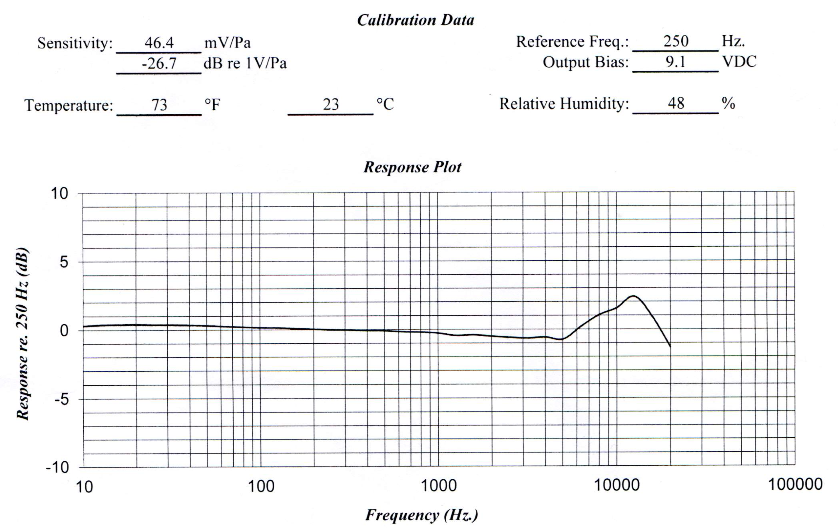
• one or more capacitive accelerometers (PCB DC capacitive accelerometer), connected to a data acquisition device (LMS SCADAS Mobile) controlled by software LMS Test.Lab;
• a professional capacitive microphone (PCB ICP microphone), connected to the same data acquisition device and controlled by the same software; an extract from its calibration sheet is presented in Figure 4;
• the factory-mounted microphone of a cellphone (Elephone P8mini with Android 7.1), controlled by a recording app (Hertz).

In each case, the tie-rod was excited using a rubber-tip, non instrumented hammer. Since any unwanted noise during the acquisition phase has a detrimental effect on the results, or at the very least leads to a longer post-processing phase, covering the hammer with some layers of soft fabric is beneficial and allows for a much clearer sound. This problem is further analysed in Section 2.5.1.

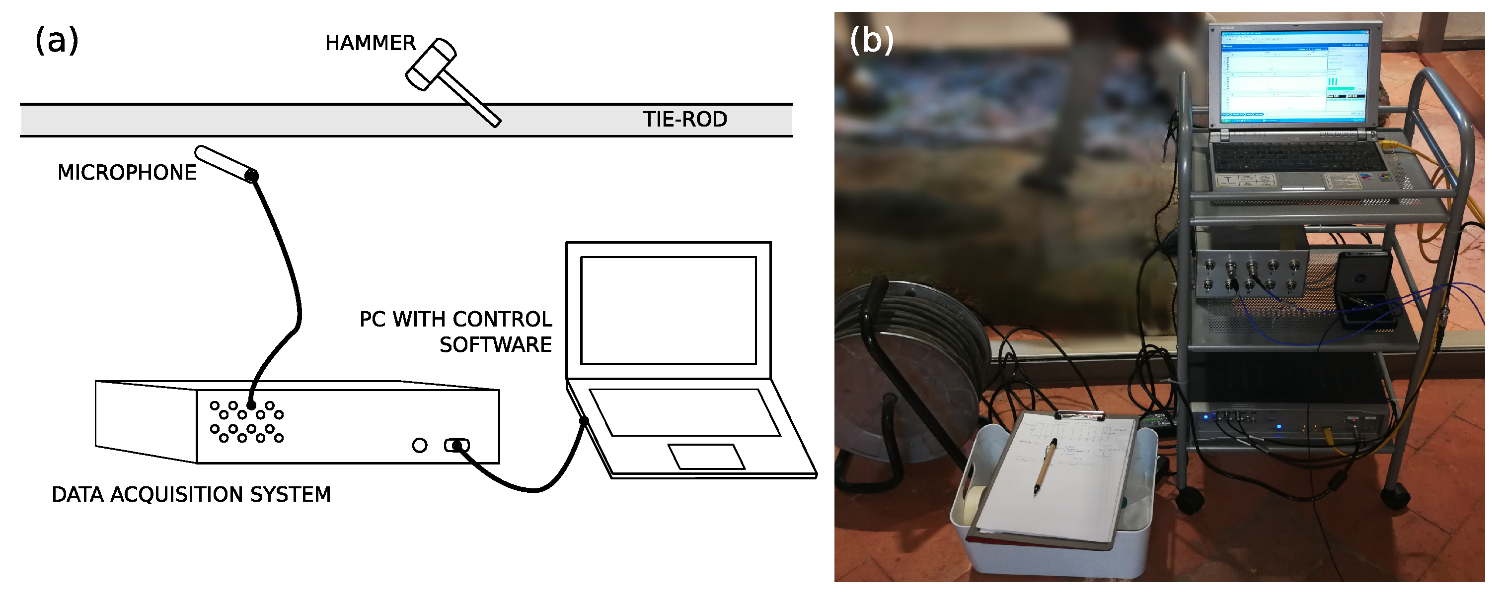
A typical professional microphone setup is detailed in Figure 5a, while Figure 5b shows the actual instrumentation (professional microphone and accelerometers) used during the testing campaign in Certosa di Pisa, which is detailed in Section 2.7.1.

For measurements with accelerometers and professional microphone, data were acquired with a sampling rate of 2048 Hz and a frequency resolution of $0.125$ Hz. The sampling rate for cellphone measurements was 8192 Hz, as the application didn’t allow lower settings.

2.4. Acquisition Procedure: Roving Input, Roving Sensor (RIRS)

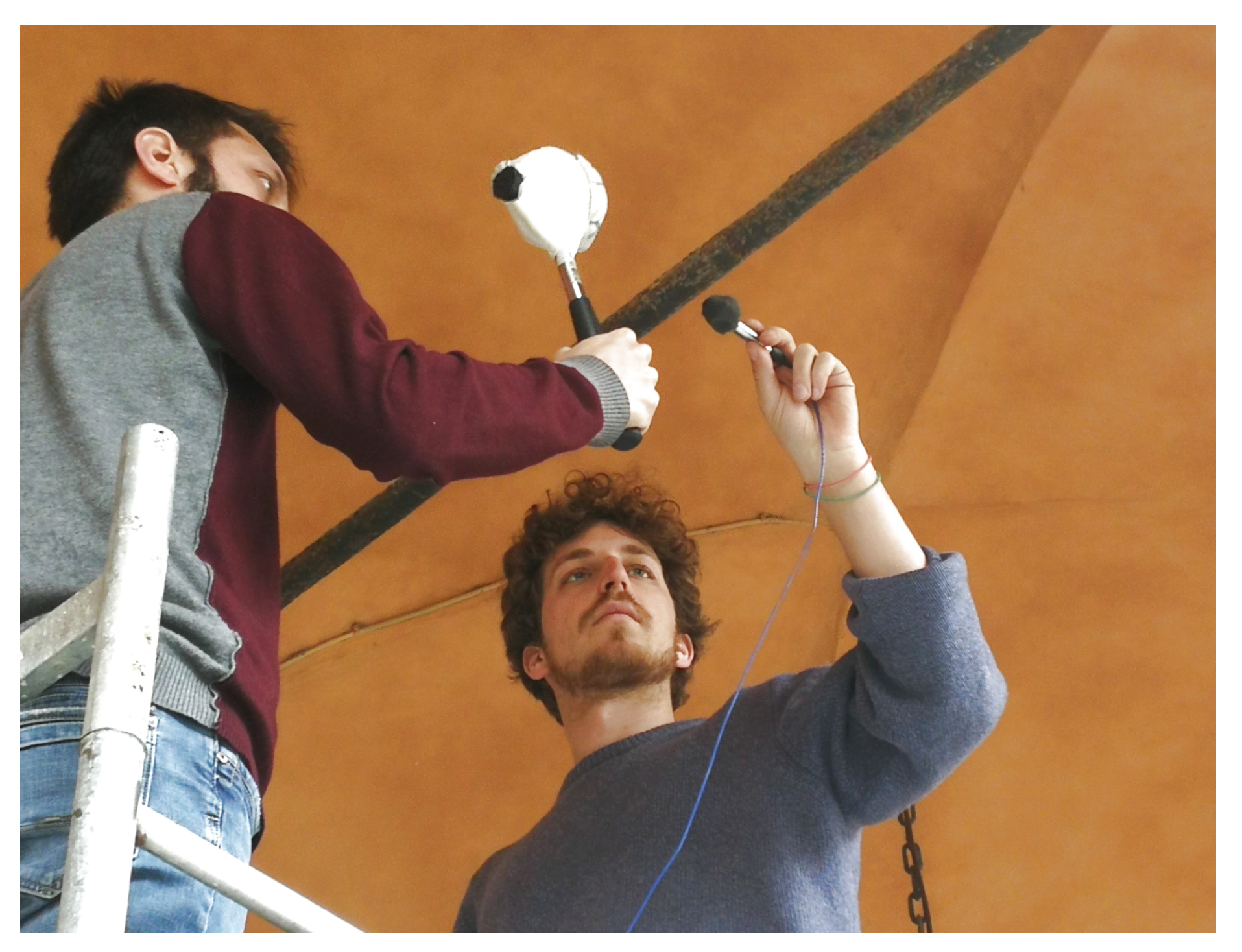
The acquisition procedure is the same with both the professional microphone and the cellphone. The microphone is placed near the tie-rod, pointed towards it, and recording is started. The tie-rod is then gently struck with the hammer, in order to produce a sound. Figure 6 shows acquisition with a professional microphone being carried out on a tie-rod in the Palazzo Arcivescovile in Pisa.

One of the required hypotheses for the application of axial load evaluation methods is that the tie-rod’s motion happens on a plane. This would actually be the case for prismatic tie-rods excited with an impulse having the same direction as one of their sections’ principal axes of inertia. In common practice, however, tie-rods are seldom devoid of torsion, and their cross-section is frequently irregular, so that identifying the principal axes of inertia would be difficult and they would differ from one cross-section to the other. Practically, it makes sense to start with input and recording aligned over a direction that the operator estimates being a good candidate for a principal axis of inertia of that section. Depending on the direction of the blow, the response spectrum may show double-headed peaks, an indication that motion has started in both principal directions, to which different resonant frequencies may belong. The measurement should then be repeated changing the direction of an angle of about 45 degrees, trying to emphasize motion in one direction over the other, and to identify which peak corresponds to which axis.

The tie-rod should be struck several times, more for noisy environments. This allows the tie-rod’s resonant frequencies to st and out in the noise, since they will be repeated with every blow during the measure, while spurious frequencies, being mostly random, have a mean closer to zero.

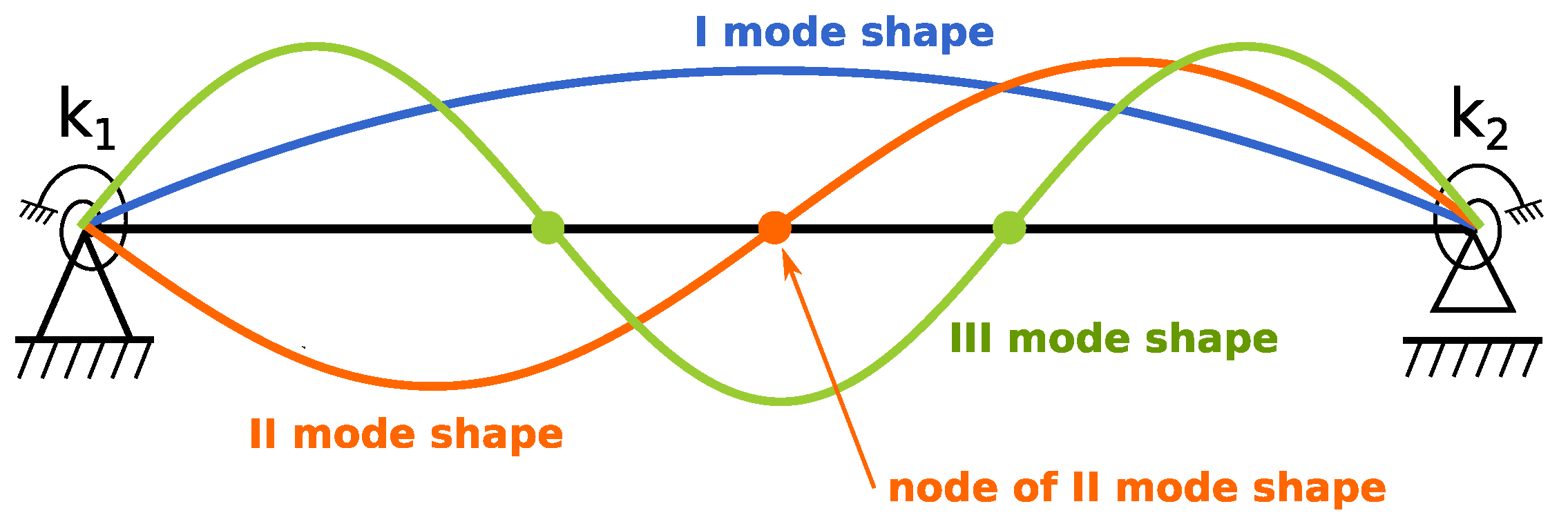
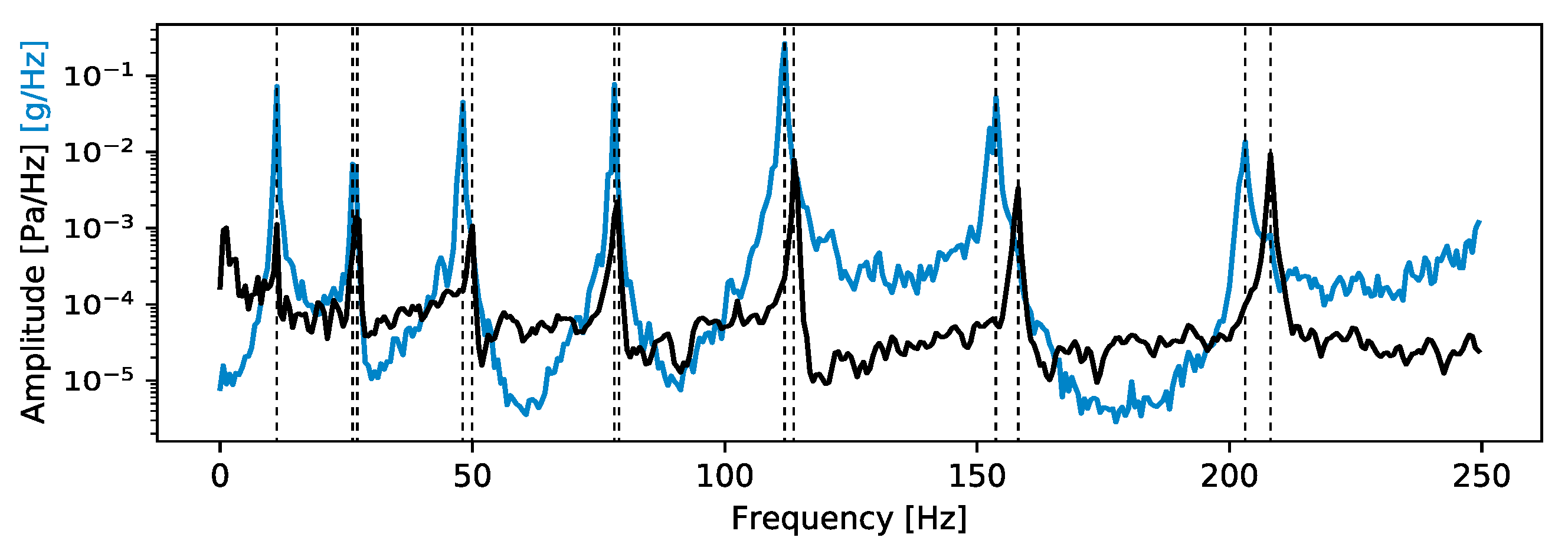
For very directional microphones some problems may arise when the sensor is placed near the tie-rod, pointed towards a node of one of its modal shapes (Figure 2). Nodes of a certain vibrational mode experience a very limited motion for the part corresponding to that mode’s frequency. The effect is that the frequency corresponding to those modal shapes is recorded with a much lesser amplitude, often making it impossible to distinguish it from the noise. Similar problems are caused by the hammer striking exactly on a node. Nodal position is a-priori unknown. 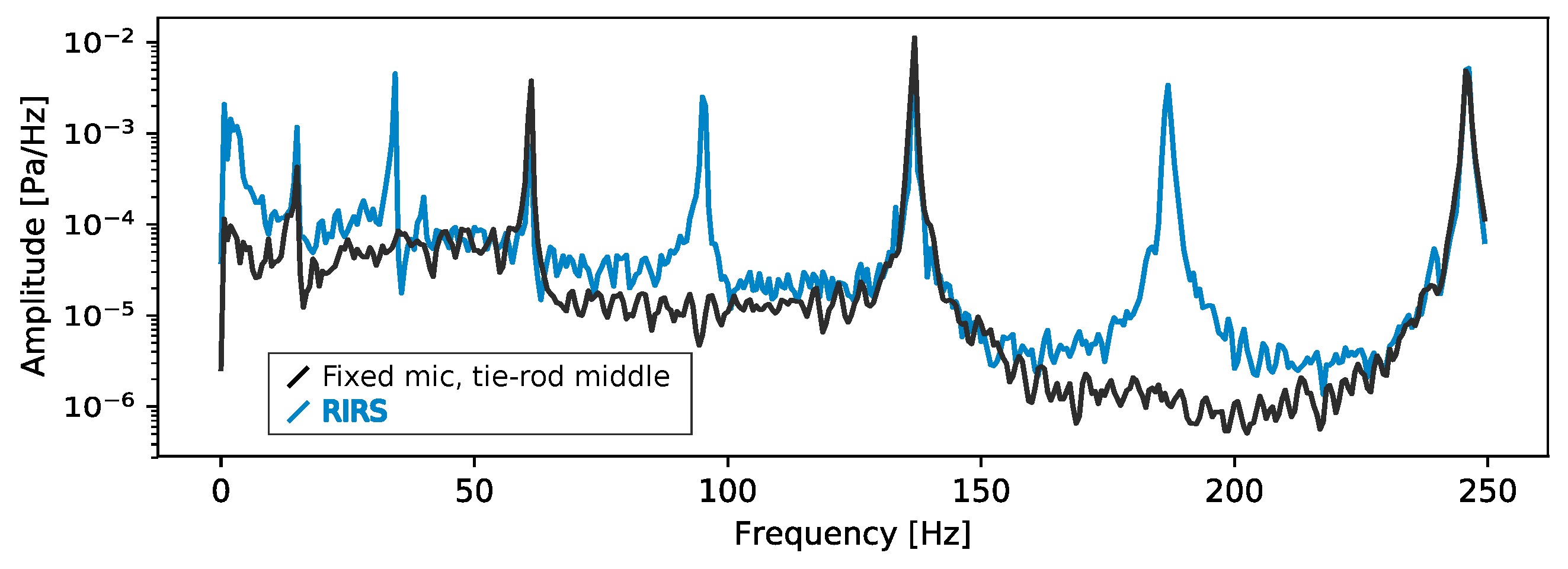The problem is solved by moving both microphone and hammer during the measurement, following a procedure here called RIRS (Roving Input, Roving Sensor). The obtained signal comprises information from inputs in multiple positions, and it is analysed as a whole. This way, even frequencies that are not evident when measuring in one position become visible in the frequency analysis of the complete signal. An example is provided in Figure 7. The black line is the Linear Spectrum of the signal obtained from measuring in the middle of the tie-rod. The lighter one corresponds to the signal obtained with RIRS. All vibration modes of even order number have a node near the middle of the tie-rod, so they cannot be identified when measuring in the middle, and thus the black line only shows odd modes. With a RIRS measurement, instead, all peaks stand out.

2.5. Digital Signal Processing

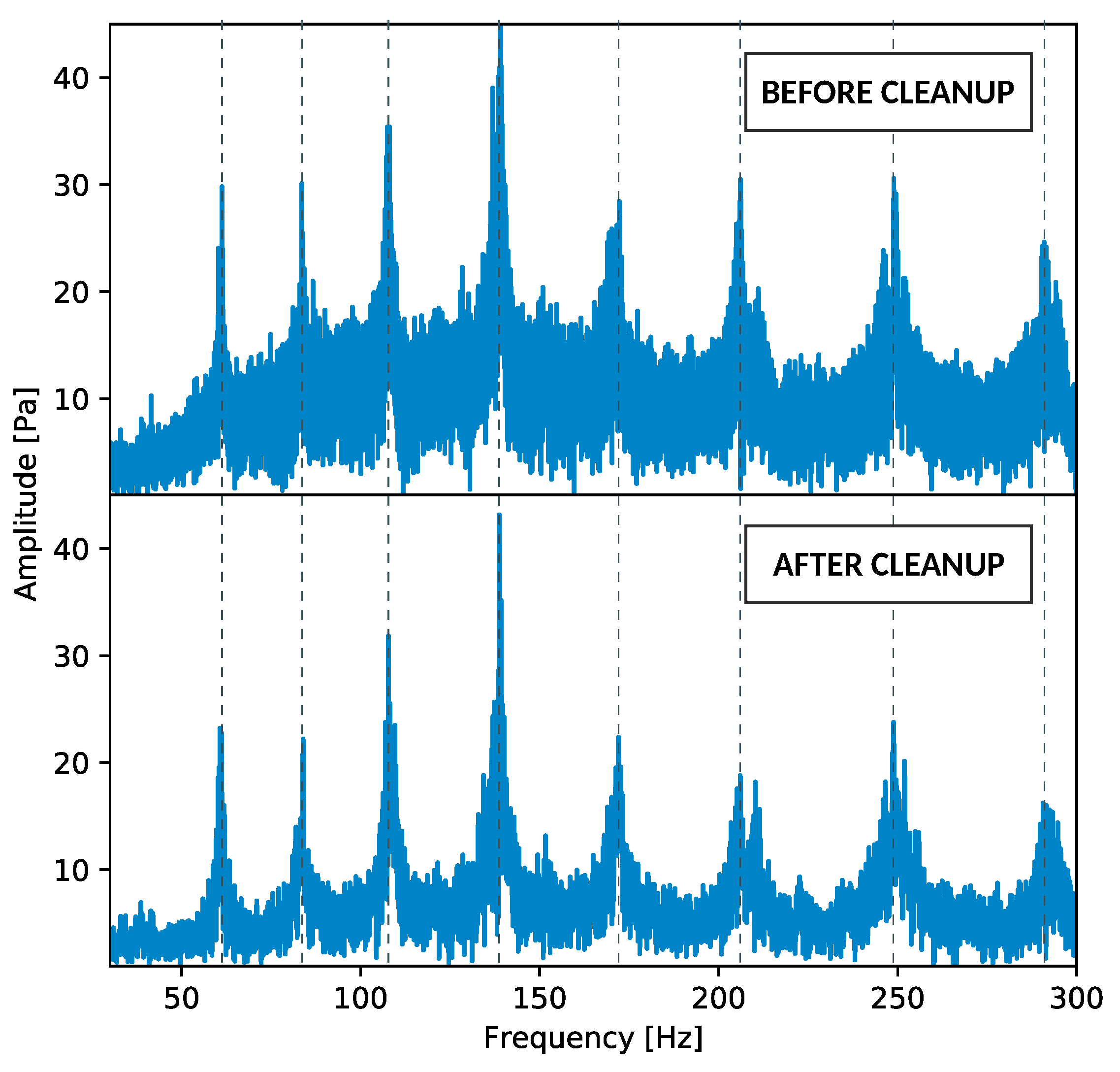
2.5.1. Manual Signal Cleanup

Having obtained the recording, a manual cleanup step may be useful before proceeding to a frequency analysis, in order to obtain a clearer result. Working with a non-instrumented hammer, the FFT of the recorded signal is used to identify the natural frequencies of the tie-rod. The hypothesis is one of free motion. Parts of the recording corresponding to hammer strikes have a spurious frequency content, since they correspond to a transient phase. They constitute a small portion of the signal, on average, so that tie-rod natural frequencies st and out nevertheless. Still, one may wish to manually delete the parts where the rod is struck. 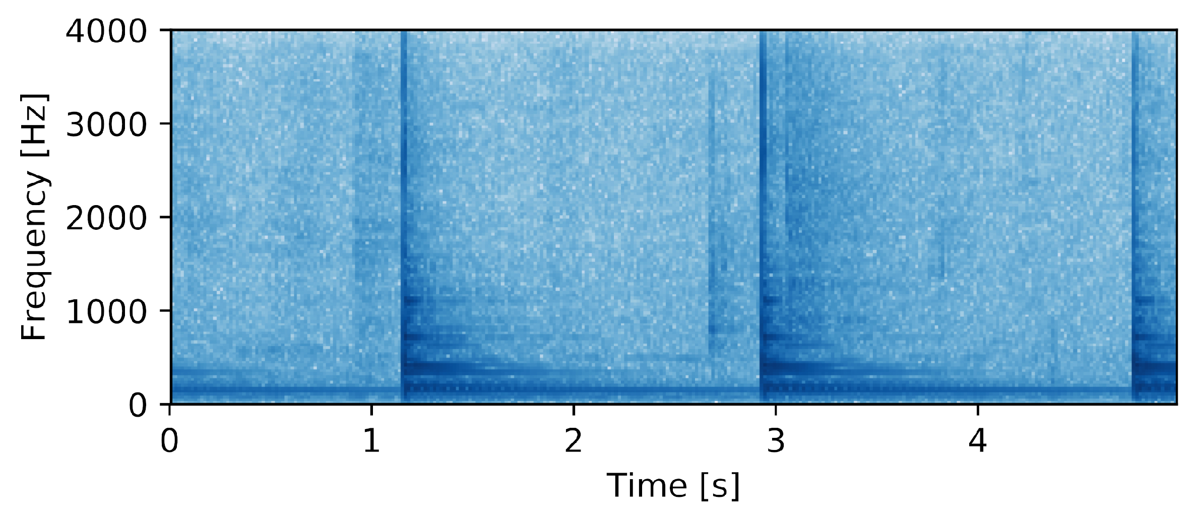To better illustrate this issue, Figure 8 shows the frequency content of a sample recording taken from one of the testing campaigns using a so-called spectrogram view. A darker colour indicates here a higher amplitude corresponding to a particular frequency at a certain time. The portion with high amplitudes ranging all the way up the spectrum corresponds to the blow. In this interval, the signal is composed by frequencies that are almost absent during the consequent free vibrations of the rod. Furthermore, eliminating portions of the signal complies with a general precautionary principle, since it doesn’t introduce new frequency content. Portions without sound between one blow and the next one may also be eliminated, since their signal-to-noise ratio is very poor.

The length of the recording is inversely proportional to smallest appreciable frequency interval. A good rule of thumb would be to have a net recording length of at least 15 s, corresponding to a frequency resolution of about 0.07 Hz.

For this research a piece of software called Audacity (which is free and open-source software, being licensed under the GNU Public License (GPL)) was used to perform the cleanup. Figure 9 shows an example of the improvement that the procedure can bring to the shape of the signal’s Linear Spectrum.

2.5.2. Frequency Analysis

The frequency content of the recorded file was analysed using its Linear Spectrum [22], as this function allows for a simple understanding of the measurement units. It was implemented using standard Python libraries.

Examples of a Linear Spectrum obtained during the present research is shown in Figure 9 and Figure 7. The natural frequencies of the tie-rod, or resonating frequencies, are the ones characterized by the highest relative amplitudes. Their identification (peak-picking) can be done either by hand, which is common practice and gives good results, or using an algorithm.

As can be seen, not all natural frequencies st and up the same way, and in noisy environments some could be very hard to identify. This problem presents also arises when using accelerometers. Fortunately, since the natural frequencies present a clear regularity, it is usually not hard for an operator to judge whether a mode is missing. Since the focus of the present work is natural frequency identification for tie-rod axial load estimation, it is worth pointing out that most techniques can be modified to work even with missing data in the frequency list. This is the case of the estimation method used in this research.

2.6. (Lack of) Lower Mode Info

Cellphone microphones, and in general microphones suited for voice recording, usually apply a high-pass filter. The microphone on the cellphone employed during this research was only able to hear frequencies over about 35 Hz. Unfortunately, the first modes of many tie-rods, such as the ones involved in the measuring campaigns presented further on, are characterized by natural frequencies lower than 25 Hz. This means that one or more of the first natural frequencies of the tie-rod, ones corresponding to the lower modes, could be missing from the recording, without any clear way to guess how many. This difficulty can be overcome through the application of a simple heuristic technique, like the one presented in this section.

Most load estimation techniques require the knowledge of some natural frequencies, without the need for them to be the first ones. The optimization step of the procedure (see Section 2.1) requires however the knowledge of each frequency’s mode order number. This would in theory rule out all acoustic measurements where the sensor’s calibration data is unknown, since it would be impossible to know how many of the tie-rod’s frequencies fall out of its operational range.

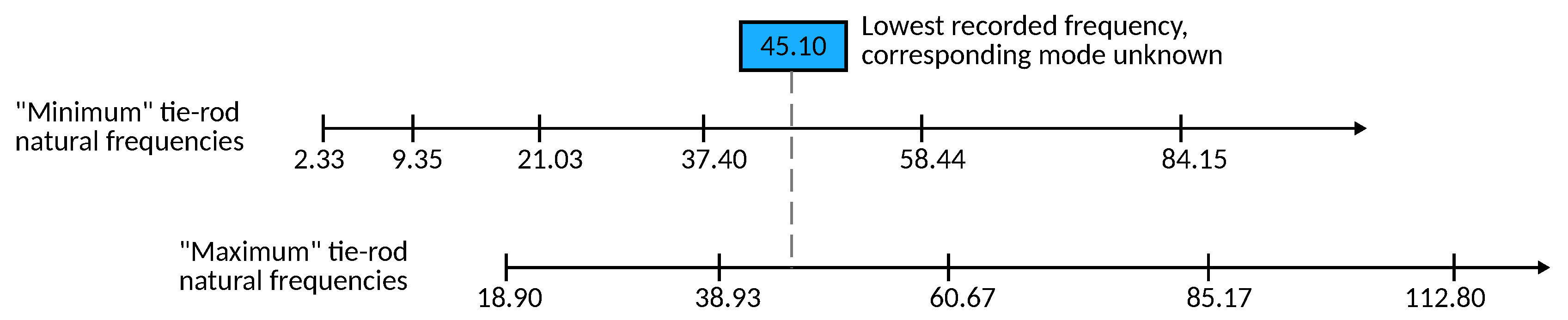
Fortunately a workaround can be found, thanks to the fact that, for each mode, natural frequencies grow higher with higher tension values in the tie-rod and with stiffer boundaries. Following the assumption of an Euler-Bernoulli beam model for the tie-rod, two extreme cases can be picked out: a minimum rod, simply supported with no axial load, and a maximum rod, with fixed end constraints and a tension equal to the mechanical resistance of the metal. The theoretical frequencies for both the minimum and the maximum tie-rod can then be calculated, knowing that the first one will show the lowest frequencies (for each mode) that the actual tie-rod can show, the other the highest. This is of course an approximation, due to the fact that the actual behaviour of the tie-rod can slightly differ from the model; still, it serves our purpose.

By comparing the lowest measured frequency with the reference minimum and maximum frequency sets, it is possible to determine an interval in which its order number is contained. The lower bound of the interval corresponds to the mode order number of the highest frequency of the “maximum” tie-rod which is still lower than the measured one. The upper bound, similarly, corresponds to the mode order number of the highest frequency of the “minimum” tie-rod which is still lower than the measured one.

Looking at the example in Figure 10, since the first four modes of the minimum tie-rod are all characterised by frequencies lower than the measured one, we can safely assume that no more than four unknown frequencies precede the measured one. In the same way, since the first two modes of the maximum tie-rod have frequencies lower than the measured one, we can decide that at least two unknown frequencies precede the measured one. So, to sum up, the first measured frequency could correspond to the third, fourth or fifth mode.

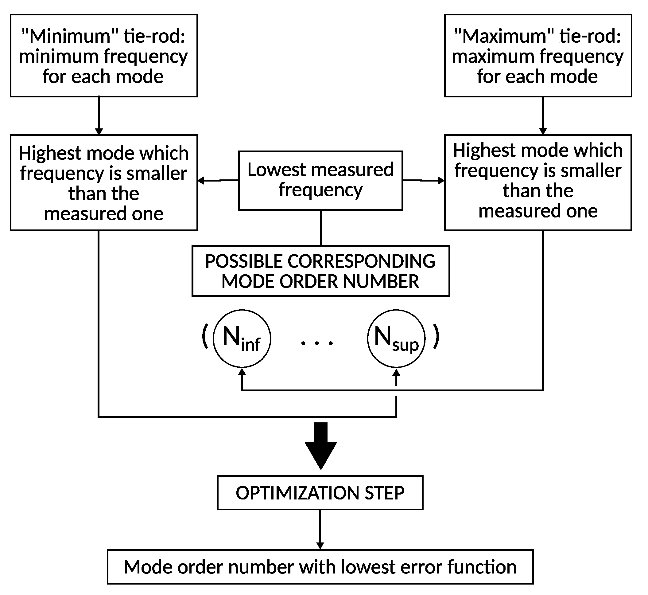
To select the right mode, the optimization should be run, and the axial load evaluated, once for every potential mode order number. Optimization functions look at all the measured frequencies and give an estimate of the axial load together with a value of the error function (see Section 2.1). Afterwards, the mode order number that leads to the lowest value for the error function is chosen. The overall procedure is summarized in Figure 11.

During the experimental campaigns, this approach has been applied to frequency measures of each of the tie-rods tested with a cellphone microphone, entrusting the algorithm to a suitable Python script. The corresponding code is provided as Supplementary Material.

2.7. Testing Campaigns

Tests to compare the results of frequency measurements with accelerometers and microphones (both professional and cellphone ones) where performed in the framework of two ongoing diagnostic campaigns carried out in Certosa di Pisa, a historical building close to the city of Pisa, in Italy, and in the Palazzo Arcivescovile, once again in Pisa. In both cases, the natural frequencies of the tie-rods were measured using one or more accelerometers (as is common practice), and a microphone. This allowed the experimenters to ascertain the fact that both instruments register the same frequency information, and to investigate the practical differences in their use. In the case of the Palazzo Arcivescovile, the tests also highlighted how the effect of having the accelerometers fixed to the tie-rod is not always negligible in terms of differences in the produced outputs.

The three different setups detailed in Section 2.3 were used in testing.

A comparison of the obtained data and consequent axial load estimate was carried out, and its results are presented and discussed in the following sections. For some of the tie-rods, several measurements with the same testing apparatus were performed. Any observed differences regarding the identified natural frequencies resulted significantly smaller than the ones corresponding to the use of different sensors. This, together with the uncertainties related to some geometrical and mechanical properties, led to the decision of disregarding measurement error at this point. A separate study is however under way, evaluating the relative influence of all significant parameters on dynamic axial load evaluation.

2.7.1. Experimental campaign in Certosa di Pisa

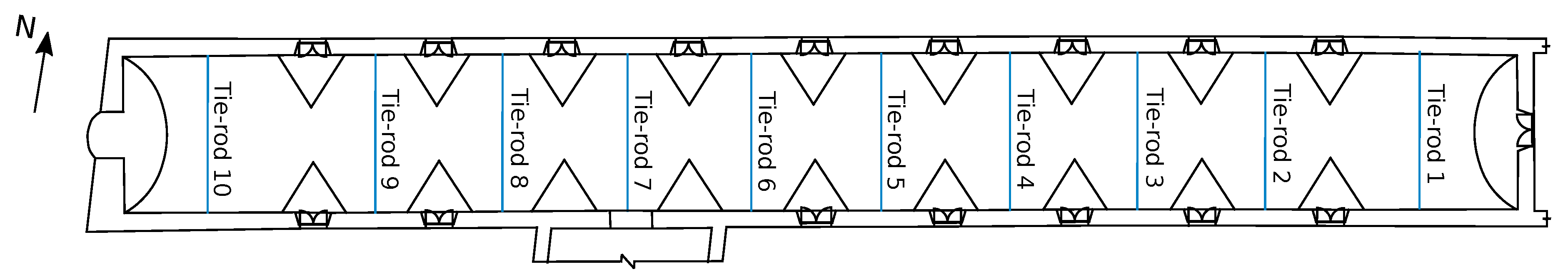
The Certosa was built over a period of centuries ranging from the 1300 s to the 1700 s, now hosting the Natural History Museum of the University of Pisa and the National Museum of the Monumental Charterhouse of Calci. The University of Pisa was recently involved in a large project concerning a complete assessment of the building aggregate of the Certosa, and in the context of static structural modelling the need arose to evaluate the tension in tie-rods of cloisters and vaulted structures. One of the investigated structures is the Galleria Barbero, an internal corridor currently hosting an exhibit. To do so, the axial load estimation technique presented in Section 2.1 was employed, and the necessary natural frequencies for each tie-rod were measured using the three different setups detailed before. This allowed to perform a comparison among the three, along with the required tension evaluation. The 10 tie-rods have roughly the same geometric properties, and since to the best of the authors’ knowledge they have all been installed in the same period, mechanical properties like Young’s modulus and density are also to be considered the same. Their quadrilateral section, though not always regular, allowed the accelerometers to be fixed by means of a magnetic base of minimum mass (about 100 g), corresponding to $0.25\%$ of the average tie-rod’s mass.

2.7.2. Experimental Campaign in Palazzo Arcivescovile (Pisa)

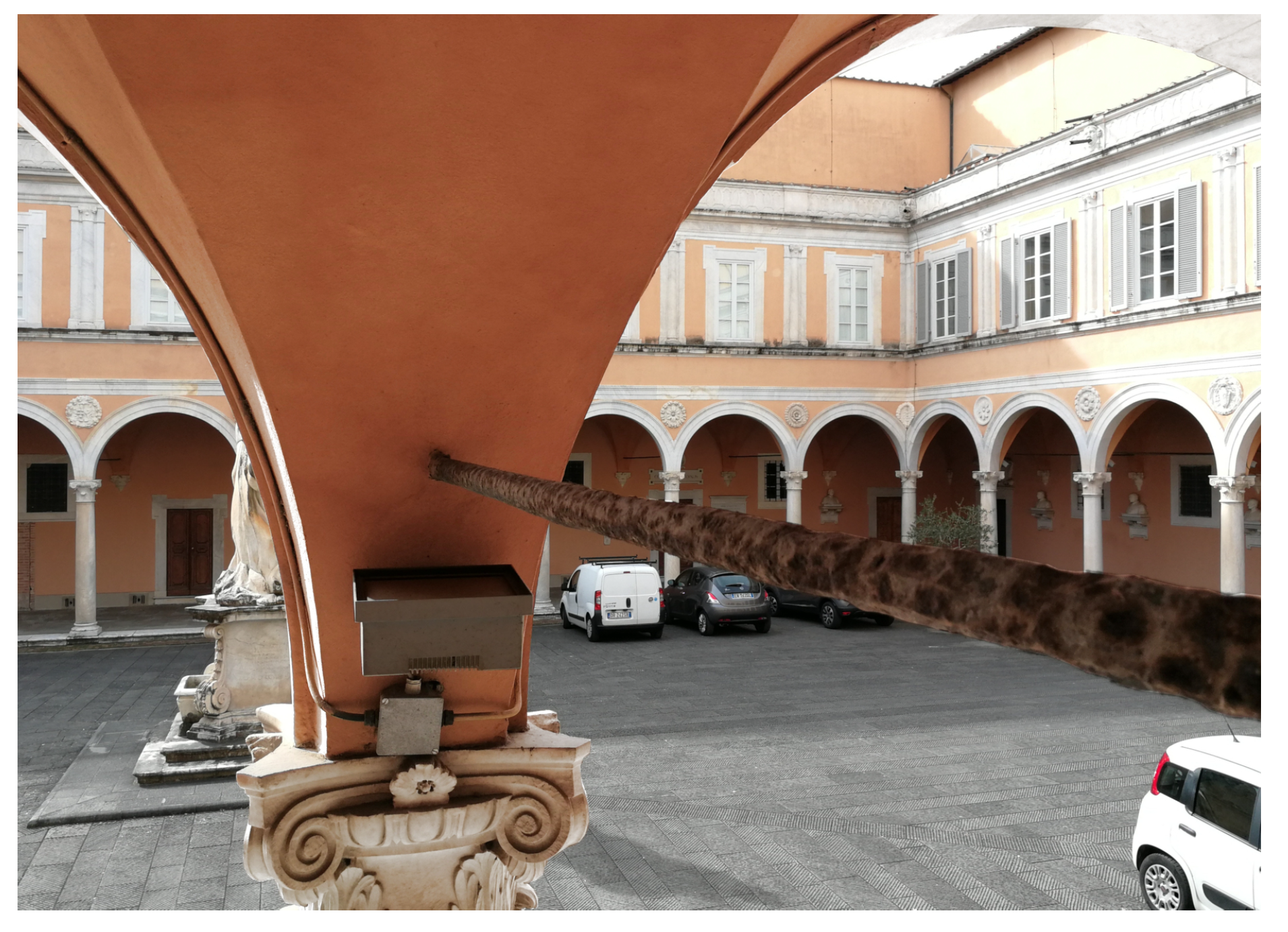
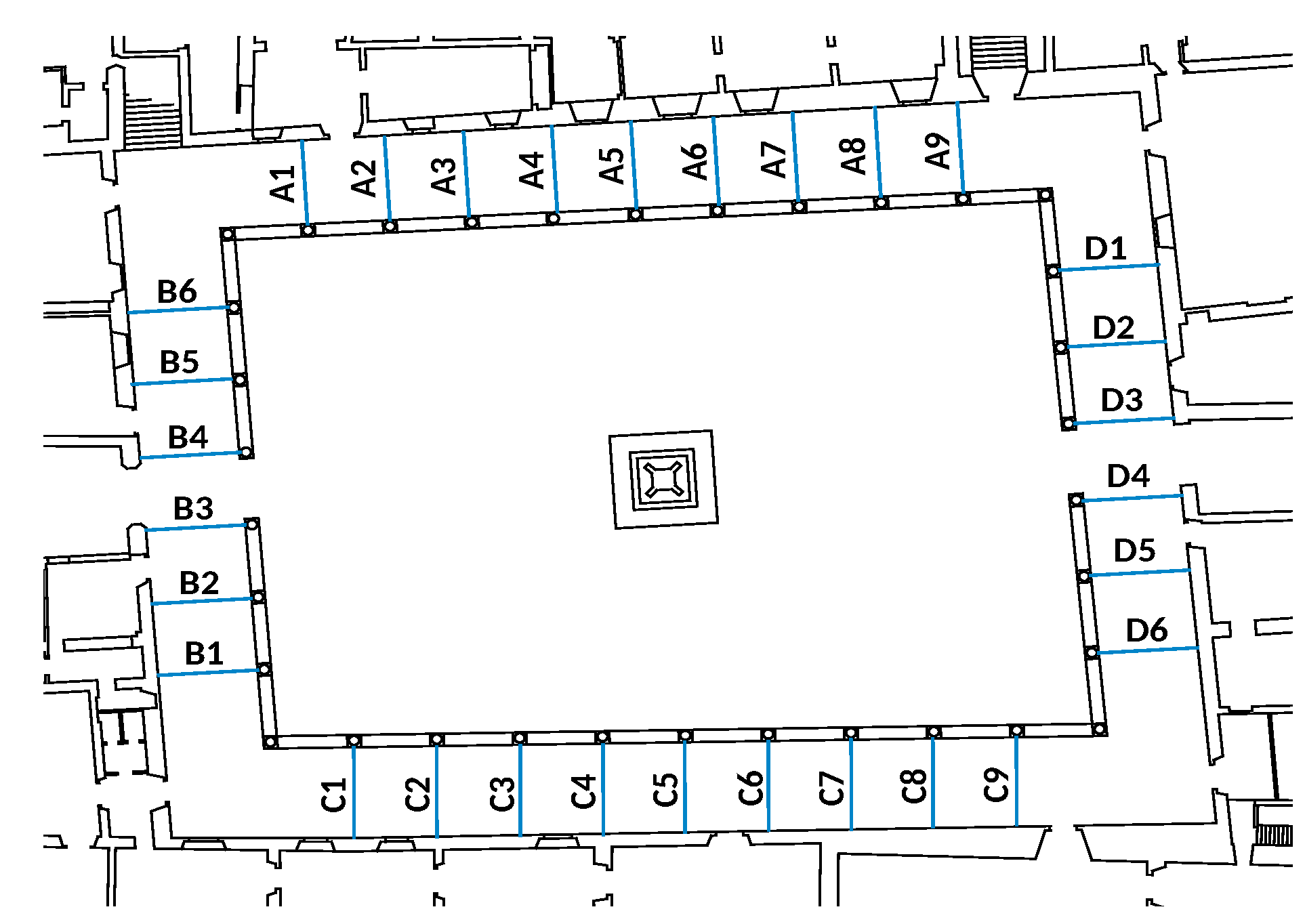
The Palazzo was mainly built during the XV century over what was left of an existing XII-century construction. The internal courtyard is surrounded by an open gallery, cross-vaulted, that comprises 30 tie-rods, about 4 m in length and with a quasi-circular section, about 3 cm in diameter (Figure 12). The actual dimensions vary slightly from one tie-rod to the other, both because of the forging process, and of a moderate corrosion.

Two of the three different setups have been used to measure the tie-rods’ natural frequencies, in the following fashion: accelerometers and professional microphone together (so that the accelerometers were mounted on the tie-rod during microphone measures), and professional microphone alone. During the former measurement, two clamps having a mass of approximately 0.55 kg each (about 2% of the tie-rod’s mass) were used to mount the accelerometers, placed roughly at the middle and at one third of the visible tie-rod’s length. Their presence resulted necessary in order to ensure a tight fixing of the sensors, since the tie-rods’ section was round and quite irregular. Testing was made difficult by the presence of wind, so a wind filter was introduced and some of the measurements were repeated.

3. Results

Results of the two testing campaigns are here given in terms of recorded frequencies. Axial loads, calculated using the estimating method presented in Section 2.1, are presented in the following Section 3.4.

3.1. Experimental Campaign in Certosa di Pisa

The results of the experimental campaign in Certosa di Pisa are here presented without reporting all the measured frequencies for each tie-rod.

Table 1. Results of testing in the Certosa di Pisa: lowest natural frequencies of the measured ten tie-rods. Values obtained with accelerometer (Acc), professional microphone (PM) and cellphone microphone (CM).

Galleria Barbero, Certosa di Pisa
Tie-Rod 1			Tie-Rod 2			Tie-Rod 3			Tie-Rod 4			Tie-Rod 5
Acc	PM	CM	Acc	PM	CM	Acc	PM	CM	Acc	PM	CM	Acc	PM	CM
11.95	12.02	-	15.12	15.18	-	11.90	11.90	-	13.11	13.11	-	11.51	11.50	-
25.62	25.49	-	31.20	30.92	-	25.57	25.57	-	27.58	27.58	-	23.99	23.96	-
41.44	41.66	-	48.89	48.68	49.3	40.85	40.85	-	43.66	43.66	43.7	38.89	39.24	39.4
61.27	61.33	-	69.39	69.67	70.1	60.14	60.14	-	62.96	62.96	63.5	57.00	57.33	57.6
83.52	83.43	85.7	92.71	92.68	94.0	81.45	81.45	82.5	85.47	85.47	85.9	78.74	78.64	79.0
111.39	111.99	113.3	120.45	120.13	121.2	107.59	107.59	108.5	111.61	111.61	111.9	104.77	104.37	104.9
Tie-Rod 6			Tie-Rod 7			Tie-Rod 8			Tie-Rod 9			Tie-Rod 10
Acc	PM	CM	Acc	PM	CM	Acc	PM	CM	Acc	PM	CM	Acc	PM	CM
12.30	12.30	-	13.51	13.51	-	12.30	12.30	-	12.70	12.70	-	12.32	12.39	-
25.97	25.57	-	28.79	28.38	-	26.78	27.18	-	26.78	26.78	-	26.01	26.55	-
41.65	41.25	41.6	45.67	45.67	45.1	42.86	42.86	-	42.46	42.46	-	42.11	41.93	-
60.95	60.95	60.5	65.37	65.37	64.8	62.15	62.15	61.9	61.75	61.75	61.1	61.84	61.36	60.9
83.46	83.46	83.0	88.69	88.29	87.8	83.66	83.66	84.1	83.86	83.86	83.5	83.17	82.81	83.2
110.00	110.00	109.9	115.63	115.63	114.2	110.00	110.00	109.9	110.14	110.00	107.8	109.74	109.93	108.7

shows the lowest natural frequencies of ten tie-rods as recorded by each sensor, in order to better illustrate the comparisons presented in Section 3.3. In all cases, the professional microphone allowed to measure the same number of natural frequencies as the accelerometer did. The cellphone microphone, instead, showed a range that didn’t extend to the lower end of the spectrum. For this reason, Table 1 only shows a reduced number of natural frequencies identified with this last sensor. Nonetheless, the measured values were used with success to evaluate the tie-rod axial load, using the method presented in Section 2.6. Figure 13 shows the disposition of the tested tie-rods in the gallery.

3.2. Experimental Campaign in Palazzo Arcivescovile

During this experimental campaign two different setups were used: accelerometer and microphone together, and microphone alone. During measurements with accelerometers and microphone together some clamps were used to fix the accelerometers to the tie-rod, as detailed in Section 2.7.2. The clamps were then removed for measurements with microphone alone. The natural frequencies obtained with the microphone during the two different measurements are presented in

Table 2. Results of testing in the Palazzo Arcivescovile of Pisa: frequency measurements for the lowest vibrational modes of 12 of the 30 tested tie-rods in the cloister. The values shown have been obtained using the professional microphone, with  and without accelerometers mounted on the tie-rod with clamps.

Internal Courtyard, Palazzo Arcivescovile of Pisa
Tie-Rod A3		Tie-Rod A6		Tie-Rod A9		Tie-Rod B2		Tie-Rod B4		Tie-Rod B6
w/ acc	w/o acc	w/ acc	w/o acc	w/ acc	w/o acc	w/ acc	w/o acc	w/ acc	w/o acc	w/ acc	w/o acc
12.40	13.01	12.68	13.18	12.91	13.68	12.25	12.80	12.69	13.02	11.70	12.06
29.29	30.17	30.10	30.87	30.65	31.09	28.45	29.11	29.15	29.81	27.72	28.38
50.90	52.88	53.65	54.42	54.27	54.93	49.43	50.64	50.67	52.73	49.58	50.84
81.77	82.10	82.87	84.52	83.53	85.07	77.79	78.39	82.46	82.79	79.60	79.71
114.08	117.71	119.48	122.82	119.63	120.45	107.03	111.98	115.61	119.02	111.80	115.76
153.06	158.58	164.61	167.69	163.73	164.61	151.85	152.40	160.43	163.62	156.10	158.08
Tie-Rod C3		Tie-Rod C6		Tie-Rod C9		Tie-Rod D2		Tie-Rod D4		Tie-Rod D6
w/ acc	w/o acc	w/ acc	w/o acc	w/ acc	w/o acc	w/ acc	w/o acc	w/ acc	w/o acc	w/ acc	w/o acc
12.61	13.05	12.4	12.84	11.61	11.96	13.47	13.93	13.93	14.51	13.54	13.77
29.37	29.92	29.3	29.85	27.93	28.39	30.92	31.61	31.49	32.18	31.15	31.92
51.8	52.9	52.08	53.4	50.05	51.66	53.97	55.35	53.85	55.35	54.08	55.58
80.81	81.41	83.67	83.67	81.44	81.55	84.96	85.19	84.96	85.07	85.56	85.56
113.92	117.33	118.3	120.94	117.03	118.99	118.09	122.46	116.71	120.85	119.44	123.01
158.45	160.78	163.17	166.25	160.94	163.43	164.89	166.73	161.56	163.51	164.27	166.93

for 12 of the 30 tested tie-rods. Figure 14 shows the tie-rod disposition in the cloister.

3.3. Comparisons between Frequency Measurements with Accelerometers and Microphone

For the full sample of tie-rods tested during both experimental campaigns, natural frequencies measured with accelerometers and with the professional microphone were compared. Values measured with accelerometers were assumed as a reference value, since accelerometers constitute the most widely used sensors for this application. The comparison was done by performing an orthogonal regression on the values, after plotting them as points on a plane of coordinates ($f_{i,Accelerometer},f_{i,Microphone}$). The ideal interpolating line, corresponding to exactly matching measures, would have a unitary angular coefficient and an intercept in the axes origin. The actual values, computed for each of the tie-rods, were observed, and their mean and standard deviation values were calculated. The resulting interpolating line has equation:

$$f_{PM}=[-0.030(\mathit{0}.\mathit{199})]+[1.000(\mathit{0}.\mathit{002})]f_{Acc},$$

(10)

where $f_{PM}$ and $f_{Acc}$ correspond, respectively, to frequencies measured with professional microphone and accelerometer, and intercept and angular coefficient values are given as $mean\left(SD\right)$.

The same procedure was followed for measurements with the cellphone microphone, on a sample of n = 10 tie-rods (the ones tested during the first experimental campaign). The resulting interpolating line has equation:

$$f_{CM}=[0.027(\mathit{0}.\mathit{755})]+[1.002(\mathit{0}.\mathit{008})]f_{Acc},$$

(11)

where $f_{CM}$ are frequency values measured with the cellphone microphone.

3.4. Comparison between Estimated Axial Loads when Measuring with Accelerometers and a  Cellphone Microphone

The efficiency of the heuristic proposed in Section 2.6 is here investigated. The algorithm was used together with the load estimation method detailed in Section 2.1 and frequency measures made with the cellphone microphone to evaluate the axial load of the 10 tie-rods of the Certosa testing campaign. In the following

Table 3. Accelerometer-Cellphone comparison: axial load estimates for the ten tie-rods in the Certosa di Pisa obtained with frequency measures from an accelerometer, or from the cellphone microphone.

Certosa di Pisa—Estimated Axial Loads
Tie-rod	Accelerometer [kN]	Cellphone [kN]	Difference [kN]	Difference [%]
1	100.60	97.69	−2.91	−2.89
2	156.55	153.64	−2.91	−1.86
3	93.71	97.84	4.13	4.41
4	113.58	124.05	10.47	9.22
5	87.57	83.67	−3.90	−4.45
6	98.06	89.14	−8.92	−9.10
7	132.21	129.91	−2.30	−1.74
8	106.43	94.30	−12.13	−11.40
9	107.59	95.43	−12.16	−11.30
10	101.79	98.90	−2.89	−2.84

, the results are compared with the ones coming from the use of the same estimation technique on frequencies measured with accelerometers.

4. Discussion

4.1. Measured Frequencies and Estimated Axial Loads

The comparison presented in Section 3.3 shows that a professional microphone and an accelerometer allow us to identify the same natural frequencies for tie-rods with sufficient accuracy. Microphones with insufficient sensitivity to low frequencies, such as the ones usually found on cellphones, may risk to miss some of the first natural frequencies. For such microphones, the heuristic proposed in Section 2.6 enables an axial loads estimate comparable to the ones obtained from frequencies measured with accelerometers. This can be seen in Section 3.4, where it is shown that using a cellphone led to errors no greater than $12\%$ during the testing campaign.

There is no rationale to decide a-priori whether a difference between frequency values or estimated axial loads is too large. Most axial load estimation methods are calibrated in laboratory or in situ. Several have also been subjected to further testing, and the results are presented in [23]. The observed errors are considered in light of their influence on the overall behaviour of the structure, and are always the subject of expert judgement.

It is important to note that no mathematical proof is given to account for the reliability of using a heuristic procedure for general purpose microphones. Conversely, it should also be clear that no measurement is complete without judgement from the operator. Considering a different number of missing modes leads, in most cases, to very different load estimates. So, should the procedure ever give an erroneous result, the operator should in turn be able to identify it.

Influence of the Sensors on the Measured Frequencies

The results presented in Section 3.2 for the Palazzo Arcivescovile testing campaign suggest the need for further discussion. For all measurements, frequency shifts can be observed between measurements performed with accelerometers and microphone, and those performed with a microphone alone. The difference is sometimes negligible for the frequency of the first mode, but it increases with higher modes reaching peaks of over 5 Hz, as is exemplified in Figure 15.

When using an accelerometer, it is necessary to fix the sensor to the tie-rod, and sometimes this may require additional instrumentation that contributes to the localized increase in mass and inertia. This was the case, for example, of the testing campaign in the Palazzo Arcivescovile. Here the mostly circular (but quite irregular) shape of the tie-rod sections rendered it necessary to employ clamps, as already detailed in Section 2.7.2.

These concentrated masses, whit their relative inertia, effectively modify the dynamic behaviour of the system, causing the sensors to measure frequencies that are no long related to the tie-rod alone.

There is no criterion to decide a-priori whether such differences are acceptable, since their influence on the evaluated axial load also depends on the geometrical and mechanical characteristics of the tie-rod, and possibly on its tension. A separate study is currently under way to assess the relative influence of several parameters on the evaluated axial load.

The presence of differences suggests that in practical cases it is best to employ a contactless measuring technique, whenever possible, and constitutes another advantage of the microphone as a sensor for this application.

4.2. Practical and Operational Differences between Different Methods

Several differences can be outlined when comparing accelerometers and microphones for the identification of tie-rods’ natural frequencies. The cost of a single microphone, even a professional one, is usually only a portion of the cost of the corresponding accelerometer. As an example, just one of the accelerometers employed during the aforementioned testing campaigns costs about 5 times the professional microphone, even though the manufacturer is the same and so are, as will be seen, the obtained results. This difference becomes extreme when considering the use of a cellphone for the measurements, since there is no need for dedicated instrumentation (not just the sensor, but the data acquisition system too) and, therefore, for any investment. The cellphone also allows a significant reduction of the time needed for testing, while the difference between the other two instruments is less noticeable, since they require a similar setup. Along time saving also comes a significantly easier mode of employ, since measuring with a cellphone only requires to start a recording application, while the presence of a data acquisition system in the accelerometer- and professional microphone setup calls for professional knowledge. The microphone is clearly only suitable to be used when performing EMA, as a audible sound has to be produced, while accelerometers can be profitably used to perform an OMA as well, making them more suitable for tie-rods that cannot be struck with a hammer, for whichever reasons.

4.2.1. Sensitivity to Wind and Other Noise Sources

One possible pitfall of the microphone is its sensitivity to environmental conditions, mainly the wind. During the second testing campaign it was observed that, even when using the professional microphone, a light breeze was enough to disrupt the acquisition of lower frequencies, due to the introduction of a great amount of noise. In the resulting signal, most of the peaks corresponding to the lower natural frequencies were undistinguishable from the noise. The problem was greatly reduced by the use of a wind filter made with a foam wrap. The same solution cannot unfortunately be applied when working in very noisy environments, and an accelerometer is in such cases the preferable choice.

4.2.2. Sensitivity to Nodes in the Tie-Rod’s Modal Shapes

Accelerometers are naturally prone to suffer the same problems outlined in Section 2.4 for directional microphones when it comes to measurements in proximity of modal shapes’ nodes. As illustrated in Figure 7, the practical effect is the impossibility to distinguish the corresponding frequency peaks. With accelerometers, the problem is traditionally solved by using two or more instruments placed in different points along the tie-rod’s axis, paying attention to avoid nodes of the same modal shape. This allows to superimpose the frequency content of the different recordings, and usually to obtain information about the first few modes. Another possibility is to attach a single accelerometer near the supports, since the intermediate nodes of the lower modes fall far enough from the tie-rod’s ends. With a microphone, the problem is solved by using the roving technique proposed in Section 2.4, without the need to employ more than one sensor, and in general to pay attention to the nodes’ position.

5. Conclusions and Further Developments

In this work, a non-destructive technique to measure a tie-rod’s natural frequencies using a general-purpose microphone, in the aim of evaluating its axial load, is proposed. The technique allows us to avoid all contact between tie-rod and sensor, and is much more simple, quick and cost-effective than other contact- or contactless methods proposed in literature. As an intermediate step, the use of a professional microphone is also described.

Measurements with cellphone microphones, where no calibration data are available, pose a problem when it comes to identifying the mode order number corresponding to each frequency. To this end, a simple heuristic approach was proposed, possibly eliminating the problem.

Two testing campaigns, making use of the aforementioned acoustic measurements, are also described, and a discussion of their results validates them and highlights the practical differences with respect to measurements with accelerometers.

Introducing the use of general-purpose microphones to evaluate tie-rod axial load would make it possible to develop a dedicated cellphone application capable of performing all the necessary analysis steps, and directly returning the final result. This would mean being able to eliminate expensive instrumentation altogether, and to create a tool that could be used for very quick assessments. As a further development, a study about the relative influence of different parameters over axial load determination is currently ongoing.