Abstract
The number of new homes built in China in 2014 doubled compared to 2004, while Korea has built more than 3000 units every year since 2004 and Japan has built more than 6000 new units. Apartments account for 60% of homes in Korea, so it is anticipated that apartment construction projects will not cease in Korea. The current company assumes that the sale rate (pre-sale rate) of apartments may be completely controlled by the pre-sale prices. The study calculated appropriate pre-sale prices to maximize the revenue of companies based on that assumption. For that purpose, the study identified the factors affecting the pre-sale prices and analyzed its correlation with the pre-sale prices based on the apartments located in Seoul, Korea. As a result of the analysis, it was found that the pre-sale prices of apartments are correlated with the number of apartment complexes, local rates, and local development level. The final result of the study suggested a way to calculate the sale prices using the factors that are thought to be correlated with the pre-sale prices. A simulation model was created using the method. When tested, it yielded an average deviation rate of 10.32%. The current study will contribute to preventing the economic losses that may be caused by apartment construction projects.
1. Introduction
The factors leading to the failure of apartment construction projects include delays in construction projects, increase in cost, and failure to achieve target pre-sale rate. According to the announcements of KOSIS (Korean Statistical Information Service), the number of new homes built in China more than doubled from 28,898 units in 2004 to 67,390 units in 2014, as shown in Figure 1, and new home construction never ceased in Korea and Japan from 2004 through 2014 [1].
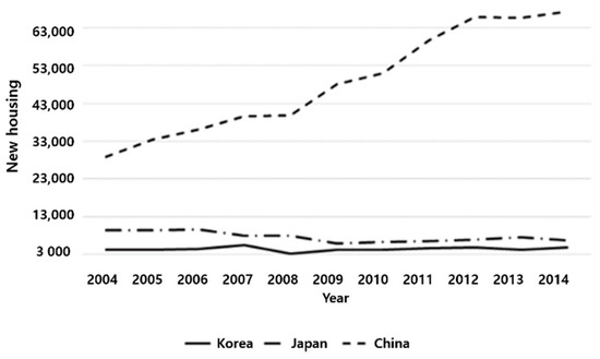
Figure 1.
Number of new housing in Korea, China, and Japan [1].
Judging by these trends, new home construction is expected to continue. In case of Korea over 60% of new homes are taken by apartments, and apartment construction projects are likely to continue. Under these circumstances, incorrect calculation of pre-sale prices for apartment construction projects can cause failure to achieve target pre-sale rates, leading to major financial losses [2]. Access to affordable housing has been a long-standing issue for households in most cities [3]. In addition, Japan experienced long-term economic depress and declivity in the real estate market after the 1990s and China may experience the same problems as Korea has, where home prices are not being adjusted due to excess vacancies caused by radical aging and macro restructuring [4,5]. Failure of apartment construction projects may have negative impacts on construction economy or lead to the bankruptcy of a company [6]. The construction economy may be depressed, causing serious social issues, including loss of jobs and the halting of construction projects [7]. Also, the incorrect calculation of pre-sale prices in the feasibility review stage may lead to false judgment of projects that are feasible. Therefore, calculating optimum pre-sale prices for apartment complexes is required for both personal and social profit [8]. In this respect, the current study suggests a way to calculate the optimum pre-sale prices considering the various factors that affect the purchase of apartments [9].
2. Literature Review
Many studies have been conducted to determine the pre-sale prices of apartments and many methods have been suggested to calculate the pre-sale prices based on the various theories mentioned above. As a result, many methods have been suggested to calculate the sale prices. Park conducted a study to calculate the appropriate pre-sale prices reflecting the market prices and buying power [10]. He identified the various factors affecting the purchase of apartments, as well as the market circumstances at the point of pre-sale, and intended to develop a model that measures the buying power and reflects it to the pre-sale price to calculate the appropriate pre-sale prices. Park derived the factors affecting new apartment purchases and surveyed the subjects to extract the purchase deciding factors. Then, the apartment sale price index announced by Korea Appraisal Board was selected as the basic data to estimate the sale price index at the point of pre-sale through time series trend analysis to use the breadth of fluctuation to derive the market prices of apartments at the anticipated point of pre-sale. Next, an AHP survey was conducted on home business experts to rate the importance of purchase deciding factors. Finally, the basic structure of pre-sale price model was established considering the market prices and buying power of apartments. After deriving the pre-sale price model, Park tested it on actual cases. He argued that the fluctuation of market price index estimated by time series was slightly different from the actual sale price fluctuation index as a result of testing the model on actual cases. He also concluded that greater buying power of projects contributes to higher contract rates and positive impact on pre-sale rates. Park expected to use the suggested model to anticipate the market at the point of future pre-sale and measure the product value of apartments and to establish the distinction/specialization strategies of businesses to reduce the risk of poor pre-sale in the unstable real estate market.
Oh used the local development level index to estimate the home demand of each region [11]. Oh focused on the fact that the Mankiw–Weil Model used to estimate the home demand cannot consider the age variations, local characteristics, and household characteristics, and the various studies conducted using it were concentrated on the metropolitan region and other certain regions. Oh classified the cities and towns in Korea into developed areas, growing areas, depressed areas, and retarded areas based on the local development level index and suggested a home demand estimation model that addresses all factors by adding the household demographics, permanent income, and housing cost to the Mankiw-Weil Model. Also, he suggested the home demand estimation model based on the population structure by age and another model applying the household structure that have mostly been used in preceding studies and introduced a model that combined the characteristics of both models. Oh used the newly developed model to estimate the home demand and concluded that the estimated home demand of retarded areas had the explanatory power of 88–90% in the population structure model, household structure model, and head of household’s age or number of household member models. He also claimed that each type’s independent variable had the significance level smaller than 0.01 and statistically valid, while the VIF value was smaller than 10 without causing any problems in terms of multicollinearity. Oh argued that all models showed differences in home demands according to the type of development level and derived that home demands varied for all types he studied. Oh expected that his study would significantly contribute to the home supply policies for certain targets, such as aged population. According to Oh, the limitations of his study were the limitations of Mankiw–Weil model and the fact that the weighted value of each index has not been updated with no further studies since 2004 and that the analysis was based on the housing survey of 2016 and the regions not sampled for the housing survey were not considered for the study.
Song surveyed the pricing behaviors of a real estate developer in Beijing, China from 2006 through 2008 [12]. They argued that the developer considers the apartments’ physical properties, the company’s financial status, and other economic circumstances to establish the apartment pre-sale prices in the early stage of pre-sale. They claimed that market fluctuation had a positive impact on the pre-sale price calculation and the developer’s pre-sale price decisions are affected by the apartment construction projects’ physical properties, the company’s financial status, and other general market conditions. They also noted that China’s government grants may affect the calculation of apartment pre-sale prices and the companies receiving grants tend to lower the sale prices and shorted the pre-sale period.
Jun studied the impact of Green Belt on the apartments of Seoul, Korea [13]. He claimed that nothing is precisely known about the impact of Green Belt on home prices. The purpose of his study was to estimate the prices related to the Green Belt reflected in the pre-sale prices of apartments in Seoul. As a result, he judged that the lease prices of high-priced leased homes located within the Green Belt are related to the geographical characteristics of Green Belt in Seoul. In case of Seoul’s Green Belt, it is located near the city center with population congestion and there are clear boundaries around it. He mentioned the possibility of his findings’ impact on the Green Belt policies in regard to the home value and claimed that the impact of Green Belt policies may significantly be affected by the geographical characteristics of Green Belt within metropolitan areas and the circumstances of Korea such as suburban patterns and housing.
3. Discussion
3.1. Deriving the Relation between Pre-Sale Prices and Pre-Sale Rate
Generally, there are various factors affecting the pre-sale rate of apartments and the impact of each factor on the sale rate (pre-sale rate) is thought to be too complicated. This concept is reflected on the study of Park to discuss various factors [10]. However, the current study suggests a different notion that the pre-sale prices can control the pre-sale rate completely. This can be proven by a simple example. Generally, the price-demand curve of apartments estimates a 100% demand with a sufficiently low price and the demand begins to decrease at a certain price and reaches 0% at another price. Therefore, the correlation between pre-sale prices and pre-sale rate is thought to be similar to Figure 2 and it would not be the maximum revenue of constructors if high sales rates are achieved with a low pre-sale price at Point A or with a high pre-sale price at Point C. The construction company can achieve the maximum revenue by achieving the target sale rate with an appropriate pre-sale price at Point B.
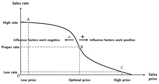
Figure 2.
Relationship between sale price and sale rate.
If the estimated pre-sale rate is low considering the above factors from a company’s perspective, it means that the apartments are not meeting the buyers’ purchase desire and the profit rate is also low. The company would need to reconsider the feasibility of business and minimize financial losses by doing so. Therefore, calculating the optimum pre-sale price would reduce the loss of construction economy, lessen the number of unsold apartment units, and prevent the bankruptcy of companies, among many other positive effects.
The current study is different from the preceding studies as stated in Figure 3. All preceding studies handled the pre-sale price as one of the many variables that affect the pre-sale rate. However, the current study assumed that the pre-sale price is the only independent variable affecting the pre-sale rate and all other variables decide the graph sale rates by sale prices. The pre-sale rate is determined by the pre-sale price only and all other variables shift the graph of estimated pre-sale rates by pre-sale prices in Figure 2 horizontally along the X axis. If each condition of an apartment complex relatively excels the condition of another apartment complex, the graph shifts to the + direction, and vice versa. In other words, buyers are likely to pay higher pre-sale prices to purchase the apartments if the apartments offer more favorable conditions, and vice versa. All other variables both shift the graph of pre-sale prices and pre-sale rates and affect each other, and the arrow means that the factor located at the start point of the arrow affects the factor located at its end point.
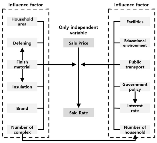
Figure 3.
Basic postulate of this study.
3.2. Deriving the General Apartment Demand Curve
The current study excerpted the study of Park to calculate the pre-sale prices of apartments [14]. Park [14] used PSM (Price Sensitivity Method) to determine the rate buyers wish to pay for national lease housing. Figure 4 indicates the results of Park’s study [14] on the correlation between the pre-sale prices of apartments and the pre-sale rates using the UTP (Unique Target Point) method. Park estimated that the cumulative probability is 0% if the price is 2424 USD per 1 m2, 50% if the price is 1985 USD per 1 m2, and 100% if the price is 1758 USD per 1 m2. The current study focused on the range where the UTP demand curve fluctuated. As a result of analyzing the graph, the demand curve showed a radical decrease in demand probability at 1858 USD per 1 m2 and only a moderate decrease from 2182 USD. The current study defines the range of radical fluctuation as the variable section.
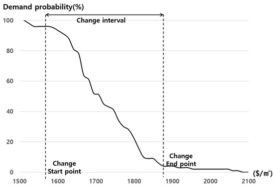
Figure 4.
Apartment demand graph using UTP (Unique Target Point).
As shown in Figure 4, the study’s apartment demand estimation curve begins to change at 1848 USD/m2 and the probability of demand derived was 95.21% when analyzed by linear regression. Also, the demand probability was 0% at 2166 USD/m2, so the variable sector of the demand curve would be from 1848 USD/m2 to 2166 USD/m2. The median of the variable section is 2007 USD/m2 and the demand probability was 47.60% as a result of the linear regression analysis. The difference between the start and end points was 317 USD/m2 and it is at 15.81% of the median, which is 2007 USD/m2. Therefore, the pre-sale prices will fluctuate within 15.81% of the median.
3.3. Correlation Analysis
Through literature review and expert advice, the current study identified the total level of apartments, number of complexes, retail and amenities, public transportation, education, underdeveloped area, and local rates as the factors affecting the apartments. Then, the study analyzed the correlation between each factor and the pre-sale prices of apartments. As there were too few samples of data from the pre-sale prices of apartments currently in the market, the pre-sale prices per m2 was surveyed for the apartments that are already sold. The study surveyed the actual prices of 70 apartments located in Gangnam-gu, Gangdong-gu, and Gangbuk-gu in Seoul that were traded in September 2019 based on the data disclosed by the Ministry of Land, Infrastructure, and Transport [15]. Also, the real estate information provided by N Website was used to survey the total level of apartment buildings, number of households, and number of complexes, which were the factors not included in the data provided by the Ministry of Land, Infrastructure, and Transport. Local underdeveloped area was surveyed by excerpting the study of Oh [11]. Oh classified the type of development level Seoul into developed, growing, depressed, and retarded as in Table 1 based on the housing survey results announced by the Ministry of Land, Infrastructure, and Transport in 2016.

Table 1.
The regional backwardness of the Seoul [15].
The unit prices (per m2) of apartments surveyed in the study and the descriptive statistics chart of each item are indicated in Table 2, and the distance to the nearest superstore from each apartment was surveyed by 0.1 km to survey the retail and amenities. In case of public transportation, the distance to the nearest station from each apartment was surveyed by 0.1 km and the walking distance to the nearest school was also surveyed by minute in case of education.
Table 2.
The selling price (per m2) and the descriptive statistical table for each.
In this study, a Pearson Correlation Cooperative (PCC) was derived using Statistical Package for the Social Sciences (SPSS) to more accurately correlate each item with the selling price per m2. PCC is a numerical representation of the linear correlation between two items, and the closer they are to 1 and −1, the more distinct they are.
The results of using (1) to correlate the selling price per m2 with each item are as shown in Table 3.
Table 3.
Correlation between the factors affecting apartment purchase and the price (per m2).
The study converted the various factors affecting each apartment into scores for the general evaluation of apartments and analyzed the correlation with the sale price per m2. For that purpose, the study divided the minimum and maximum values of each item by 10 to rate each item between 1 and 10 (Appendix A).
As a result of applying PCC of the unit price per m2 for the comprehensive evaluation of each item, the correlation was 0.71 and significant, while the distribution of scores and unit prices per m2 clearly showed that the sale prices per m2 increased with greater comprehension scores as in Figure 5.
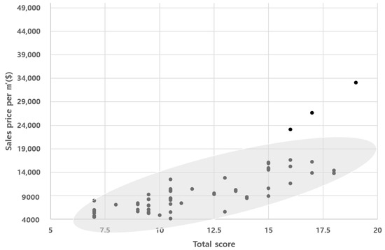
Figure 5.
Scatter diagram of total score and sales prices per m2.
Then, the study applied the number of apartment complexes, local rates, and local development level with prominent correlation with the sale price per m2 to derive correlation. Figure 6 indicates the comprehensive scores of the number of apartment complexes, local rates, and local development level and the dispersion of sale prices of apartments per m2. PCC using Equation (1) was 0.83 and higher than 0.71, which was the weighted value when all the items were applied.
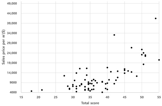
Figure 6.
Scatter plot of total score correlated factors and sales prices per m2.
Data dispersion was not very wide comparing the dispersion of comprehensive scores of all items of Figure 5 and the sale prices per m2, manifesting that the current study’s method of calculation was more reliable. Later, the correlation with the unit price per m2 was derived by applying the weighted value of each item to the scores of the number of apartment complexes, local rates, and local development level as in Figure 7. Considering the importance of each item, the weighted values were 0.25, 0.50, and 0.25, respectively.
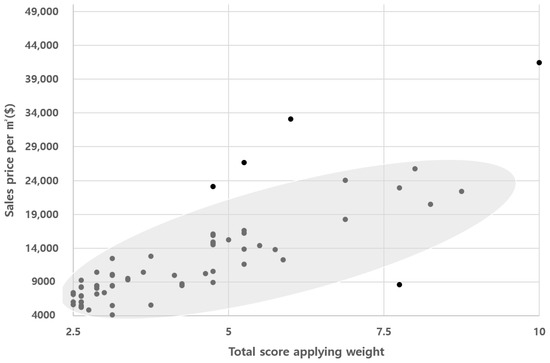
Figure 7.
Scatter plot of total score correlated factors and sales prices per m2 applying weight.
In that case, PCC was 0.83 and greater than 0.77, which was PCC when the weighted values of all items were applied, and the correlation was greater. This means that the study’s reliability was higher as with the scores that did not apply the weighted values.
3.4. Development of Pre-Sale Price Calculation Simulation Model
The current study suggested the following method to calculate the pre-sale prices that yield the greatest profit to companies.
First, the A value was set as the base price of pre-sale. The current study collected data from Seoul, so the A value was the mean sale price of Seoul. The mean pre-sale price of private apartments currently on sale in Seoul was 9651 USD per m2 and not very different from 9879 USD per m2, the mean pre-sale price of apartments sold. In order to acquire more data, the study applied the mean sale price per m2, not the mean pre-sale price per m2, as the base price of apartments as the data of apartments sold at similar periods, not the apartments currently in the market, reflect prices not affected by market.
Second, the start and end points of fluctuation, which mark the range of variable section based on the A value, were determined as in Figure 8. As a result of examining the existing literature in Section 3.2, it was derived that the range of variable section was 15.8% based on the A value. The pre-sale rate was 100% at the start point of fluctuation, so any pre-sale rate lower than the start point would only lower the pre-sale prices while maintaining 100% pre-sale rate. Therefore, it is meaningless to set the pre-sale price at any point below the start point of fluctuation, so the start point of fluctuation will be the minimum (min) of pre-sale prices. In case of the end point of fluctuation, the pre-sale rate will stay at 0% with any pre-sale prices greater than it. Therefore, the end point of fluctuation becomes the maximum (max) of pre-sale prices. Then, the pre-sale rate graph will be drafted according to the pre-sale prices that yield 100% pre-sale rate at the start point of fluctuation and 0% at the end point of fluctuation. The current study evaluated each factor on a scale of 1 to 10, so the score when the pre-sale price is the A Value is the price when the score is 5.5 points.
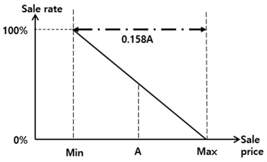
Figure 8.
Set value.
Third, each factor was evaluated and scored and to multiply the scores by each factor’s weighted value to derive the comprehensive score as in Figure 9. The pre-sale rate graph by pre-sale prices was shifted left or right according to the comprehensive score. In other words, the pre-sale rate graph by sale prices is drawn where the start point of fluctuation shifts from min to min’ and the end point of fluctuation shifts from max to max’ with 100% pre-sale rate at min’ and 0% pre-sale rate at max’.
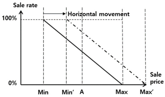
Figure 9.
Horizontal movement of graphs according to itemized.
Finally, the X value is derived, the product of pre-sale price and pre-sale rate from the final graph in Figure 10. The companies cannot reach the target profit when the pre-sale rate is raised with excessively low pre-sale prices or the pre-sale rate is lowered with excessively high sale prices, so incorrect calculation of pre-sale prices leads to great economic losses. Therefore, it is important to calculate the appropriate pre-sale prices that yield the greatest profit to the companies as the X value and the current study developed the following simulation to find it.
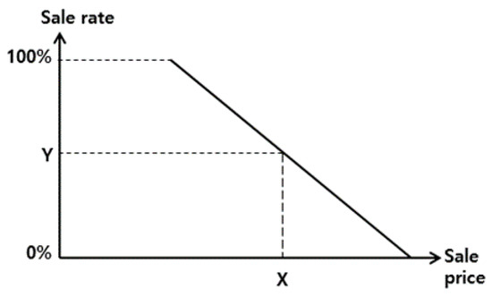
Figure 10.
Elicitation of pre-sale price.
The current study developed the simulation model shown in Figure 11 based on the method of calculation of pre-sale prices. The simulation model was Powersim.
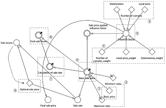
Figure 11.
Developed simulation model.
First, the base value could be entered in ① to set the base of pre-sale price. The current study entered 9,879,000 KRW, the mean sale price of Seoul in September 2019. Then, the rate could be entered in ② to set the start and end points of variable section based on the base price in ① [16]. The current study set the range of variable section at 15.8% of base price and the minimum rate and maximum rate were 7.9%, which was 1/2 of 15.8%, thus 0.92 and 1.08, respectively. Also, the pre-sale rate was set to start at 100% with the minimum rate and decrease down to 0% at the maximum rate after through gradual decrease in reverse proportion to the pre-sale price. Then, the score of each factor could be entered in ③ and the weighted value of each factor in ④. As a result of regression analysis of the correlation of weighted scores of the number of apartment complexes, local rates, and local development level and the sale price per m2, the formulas in (2)–(4) were derived:
In other words, the pre-sale price of apartments increased by 3422 USD when the weighted score of the number of apartments complexes increased by 1, while it increased by 4143 USD when the weighted score of local rates increased by 1. In the case of local development level, the weighted value was 10.0 for developed, 7.5 for growing, 5.0 for depressed, and 2.5 for retarded. As the weighted value was 0.25 for retarded, the score increased by 0.625 when development level increased by level 1. When this was applied to (4), the price increased by 2892 USD when development level increased by level 1. ⑤ applied this to simulation and shifted the graph left or right according to the weighted score of each factor. Through this process, the simulation derived graph of pre-sale rate according to the pre-sale prices in ⑥. ⑦ visualizes the pre-sale rate corresponding to each sale price and the simulation system calculates the pre-sale income as in ⑧ by the product of ⑥ and ⑦. Then, the optimum sale price is derived as in ⑨ for the maximum pre-sale income. For that purpose, ⑧ was set as the target function and ⑨ was the decision-making variable. Optimization search is conducted based on the evolution search algorithm to search the optimum value of optimum sale prices to maximize the pre-sale income. The simulation was applied to derive the pre-sale price per m2 when the scores of all factors were 5.5 and Figure 12 indicates the sale prices derived from each time of simulation. The time of simulation is defined as one shift of graph by 1/100 from the start of fluctuation to the end of fluctuation when the start point was 0 and the end point was 100. In other words, n times of simulation simulates the shift of graph by 1/100 n times from the start of fluctuation to the end of fluctuation. The pre-sale price per m2 increased gradually from the start point to the end point. Also, the simulation set all scores at 5.5, so the sale price per m2 at 50th simulation 9879 USD, which was the mean sale price of Seoul.
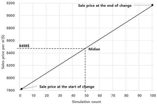
Figure 12.
Pre-sale price according to the time of simulation.
Figure 13 shows the pre-sale rate according to the time of simulation. The sale price increased from the start point to the end point, so the pre-sale rate decreased in reverse proportion and reached 50% at 50th simulation. The pre-sale income increases in proportion to the exclusive area and number of units, so the current study ignored these factors and set the pre-sale income as the sale price per m2 multiplied by the pre-sale rate.
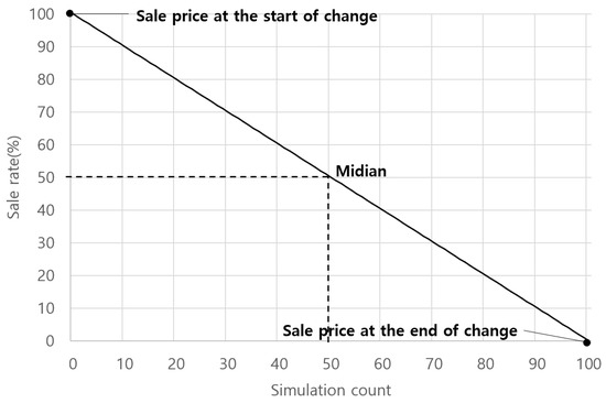
Figure 13.
Pre-sale rate according to the time of simulation.
The pre-sale income of apartments according to each sale price is as indicated in Figure 14. The pre-sale income graph according to sale prices drew a curve of moderate declivity. The pre-sale rate was 100% when the sale price was 9089 USD for the highest pre-sale income of 9089 USD, and this means that the optimum sale price of apartments was 9089 USD.
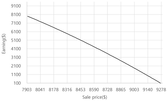
Figure 14.
Pre-sale income of apartments according to each sale price.
After the simulation, the study additionally adjusted the coefficient that becomes the standard of weighted score of each factor. Previously, each factor was evaluated on a scale of 1 through 10, so the median of 5.5 was multiplied by 0.50, 0.25, and 0.25, which are the weighted values of local rates, local development level, and the number of apartment complexes, respectively, for the simulation of range of fluctuation derived by applying 2.75, 1.38, or 1.38. As a result of the simulation, there was a large error between the estimated pre-sale prices and the actual sale prices when the standard values were used, so the current study adjusted the standard value of each item to 1.01, 1.94, or 0.85 to finalize the simulation. The results of estimating the sale prices based on the simulation of apartments sold are in Table 4. The minimum error rate of simulation was 0.12% and the maximum error rate was 24.71% with a standard deviation of 10.32% as a result of the simulation. When compared to the previous simulation, the adjusted simulation reduced the error between all apartments’ actual sale prices and the results of simulation.
Table 4.
The error rate and deviation rate of the simulation.
As a result of the simulation, there were apartments whose appropriate sale prices were lower or higher than the actual sale prices. In the case of the apartments whose appropriate sale prices were higher than the actual sale prices, it is assumed that the apartments were traded at lower prices because the buyers overlooked the outstanding environment and value of apartments traded. On the other hand, the apartments whose appropriate sale prices were lower than the actual sale prices were probably traded due to overestimation of the actual apartments based on the buyers’ personal value.
The simulation developed by the current study is expected to contribute to increasing the profitability of apartment constructors and preventing economic losses. However, the study had a few limitations. First, it is the limitation of survey data. The current study was conducted to examine the correlation between various factors and the sale price per m2 of apartments. The study surveyed 70 apartments sold in Seoul in September 2019, but the factors selected in the study were not significantly correlated with the sale price per m2 except for a few. This is probably because the number of data gathered for the study were scarce, so a greater pool of data would be needed to draw the conclusion that many items affect the sale price per m2. The current study could not consider the special variables such as the speculators. Therefore, the simulation of the study could be improved if more factors affecting apartments are selected in future studies.
Second, it is the weighted values of factors. The study selected seven factors affecting the sale prices of apartments to set the weighted values. However, the factors with no correlation were excluded along the course of study to make it impossible to set the accurate weighted value for each factor. For that reason, the study assigned random weighted value to each factor and it had significant impact on the results of study. Therefore, it would be possible to calculate the sale prices close to the optimum sale prices when accurate weighted values are derived from future studies.
Finally, it is the incorrect range of variable section. The study excerpted a preceding study to set the range of fluctuation of presale rate estimation curve according to sale prices. As a result, the range of variable section was set at 15.8% based on the base price. This value is realistically too small to change people’s purchase desires, so an accurate range of variable section would be able to derive more reliable sale prices through future studies.
4. Conclusions
The current study examined the method of calculating the optimum sale prices to enhance the capacity of feasibility review in prior to apartment construction projects and to prevent the economic losses of construction industries. This type of study has been attempted using various methods, but there were various limitations. In order to overcome the limitations, the current study derived the correlation of each factor and the sale price and developed a simulation model to calculate the sale prices of apartments. The preceding studies handled the sale prices of apartments as one of several factors of business, but the current study assumed that it is the only factor affecting the pre-sale rate. Also, it was theorized that other factors besides the sale prices are the factors changing the pre-sale rate estimation graph according to the sale prices of apartments. Based on the theory, the study derived the pre-sale rate-demand estimation curve according to the sale prices of apartments by excerpting a preceding study prior to calculating the appropriate sale prices of apartments. The study defined the variable section by deriving the sale prices where the fluctuation of pre-sale rates starts and ends on the derived graph and derived the characteristics of variable section. After that, the factors affecting the purchase of apartments included seven factors, including the total level of apartments, number of complexes, distance to superstores, distance to stations, distance to schools, local rates, and development level. Then, the sale prices per m2 and the factors affecting the purchase of apartments were surveyed for 80 apartments traded in Seoul as of September 2019. After that, the correlation between each factor and the sale price per m2 was derived using PCC (Pearson Correlation Coefficient). As a result, it was found that all factors except for the number of complexes, local rates, and local development level had no correlation with the sale price per m2. Therefore, the study applied the number of complexes, local rates, and local development level to calculate the sale prices of apartments. For that purpose, each factor was rated on a scale of 1 to 10 to tabulate the comprehensive score of each apartment. The current study applied the weighted value of each factor to readjust the comprehensive scores to derive the correlation with the sale price per m2 to enhance the accuracy of study. PPC of weighted scores and sale prices per m2 was 0.83, manifesting that the correlation between the two factors was very high.
Based on the results, the study developed a simulation system to calculate the appropriate sale prices of apartments. For that purpose, the study summarized the pre-sale price calculation method as follows: first, local rates were the base prices of apartments. Then, the width of variable section was established and set at 15.8% based on the local rates. Then, the variable section was shifted horizontally according to the score and weighted value of each factor and the sale price for maximum product of sale price and pre-sale rate was derived from the pre-sale rate graph based on the final sale prices. The study developed a simulation model for this and calculated the sale prices of apartments to conclude that the pre-sale rate was 100% with the minimum sale price at the start point of fluctuation to maximize the sale income.
The study calculated the appropriate sale prices of apartments for maximum profitability of companies and is expected to contribute to preventing the economic losses for companies and to providing consumers with the list of apartments suitable for the sales prices they would pay. However, the study had several limitations, including the fact that there were limited data to derive accurate correlation between various factors and sale prices per m2, the fact that the weighted value of each factor was inaccurate, and the fact that there was not enough study was set the range of variable section. With follow-up studies to overcome the limitations, appropriate pre-sale prices will be calculated more accurately.
Author Contributions
Conceptualization, K.K. and D.L.; methodology, K.K.; software, K.K.; validation, K.K., J.Y. and S.K.; formal analysis, K.K.; investigation, J.Y.; resources, K.K.; data curation, J.Y.; Writing—Original draft preparation, K.K.; Writing—Review and editing, J.Y., K.K., S.K., D.Y.K. and D.L. All authors have read and agreed to the published version of the manuscript.
Funding
This work was supported by the National Research Foundation of Korea (NRF) grant funded by the Korea government (MSIT) (No. 2020R1C1C1012600).
Conflicts of Interest
The authors declare no conflict of interest.
Appendix A. Score Range by Item
| Score | Total Number of Floors in Apartments | Number of Complexes | Retail and Amenities | Public Transportation | Educational Environment | Local Rates |
|---|---|---|---|---|---|---|
| 10 | 62.6 ≤ A | 46 ≤ B | 0.1 ≤ C ≤ 0.26 | 0.2 ≤ D ≤ 0.33 | 1 ≤ E ≤ 2.6 | 30,572 ≤ F |
| 9 | 56.2 ≤ A < 62.6 | 41 ≤ B < 46 | 0.18 < C ≤ 0.26 | 0.33 < D ≤ 0.46 | 2.6 < E ≤ 4.2 | 27,763 ≤ F < 30,572 |
| 8 | 49.8 ≤ A < 56.2 | 36 ≤ B < 41 | 0.26 < C ≤ 0.34 | 0.46 < D ≤ 0.59 | 4.2 < E ≤ 5.8 | 24,954 ≤ F < 27,763 |
| 7 | 43.4 ≤ A < 49.8 | 31 ≤ B < 36 | 0.34 < C ≤ 0.42 | 0.59 < D ≤ 0.72 | 5.8 < E ≤ 7.4 | 22,146 ≤ F < 24,954 |
| 6 | 37.0 ≤ A < 43.4 | 26 ≤ B < 31 | 0.42 < C ≤ 0.50 | 0.72 < D ≤ 0.85 | 7.4 < E ≤ 9 | 19,337 ≤ F < 22,146 |
| 5 | 30.6 ≤ A < 37.0 | 21 ≤ B < 26 | 0.5 < C ≤ 0.58 | 0.85 < D ≤ 0.98 | 9 < E ≤ 10.6 | 16,528 ≤ F < 19,337 |
| 4 | 24.2 ≤ A < 30.6 | 16 ≤ B < 21 | 0.58 < C ≤ 0.66 | 0.98 < D ≤ 1.11 | 10.6 < E ≤ 12.2 | 13,719 ≤ F < 16,528 |
| 3 | 17.8 ≤ A < 24.2 | 11 ≤ B < 16 | 0.66 < C ≤ 0.74 | 1.11 < D ≤ 1.24 | 12.2 < E ≤ 13.8 | 10,911 ≤ F < 13,719 |
| 2 | 11.4 ≤ A < 17.8 | 6 ≤ B < 11 | 0.74 < C ≤ 0.82 | 1.24 < D ≤ 1.37 | 13.8 < E ≤ 15.4 | 8102 ≤ F < 10,911 |
| 1 | 5.0 ≤ A < 11.4 | 1 ≤ B < 6 | 0.82 < C | 1.37 < D | 15.4 < E | 5293 ≤ F < 8102 |
References
- G20 New Housing Status, Korean Statistical Information Service (KOSIS). 2017. Available online: https://kosis.kr (accessed on 1 March 2020).
- Hong, L.H.; Lee, M.H. An Analysis of the Importance of Housing Indicators for the Evaluation of the Housing Sale. J. Resid. Environ. Inst. Korea 2020, 18, 319–332. [Google Scholar] [CrossRef]
- Ezebilo, E.E. Evaluation of House Rent Prices and Their Affordability in Port Moresby, Papua New Guinea. Buildings 2017, 7, 114. [Google Scholar] [CrossRef]
- Woo, A.; Joh, K.; Yu, C.Y. Who believes and why they believe: Individual perception of public housing and housing price depreciation. Cities 2020, 1–13. [Google Scholar] [CrossRef]
- Son, S. A Simulation Model for Feasibility Analysis of Apartment Building Projects Using System Dynamics. Master’s Thesis, Kyung Hee University, Seoul, Korea, 2018. [Google Scholar]
- Kim, J.M.; Son, K.; Jang, J.; Son, S. Development of an income and cost simulation model for studio apartment using probabilistic estimation. J. Asian Archit. Build. Eng. 2020, 1–10. [Google Scholar] [CrossRef]
- Huh, Y.K.; Hwang, B.G.; Lee, J.S. Feasibility Analysis Model for Developer-proposed Housing Projects in the Republic of Korea. J. Civ. Eng. Manag. 2012, 18, 345–355. [Google Scholar] [CrossRef]
- Baik, M.S.; Shin, J.C. A Study on the Determinants of Initial Sales Rate for New Apartment Housing. J. Korean Urban Manag. Assoc. 2011, 24, 213–237. [Google Scholar]
- Kim, Y.; Choi, S.; Yi, M.Y. Applying Comparable Sales Method to the Automated Estimation of Real Estate Prices. Sustainability 2020, 12, 5679. [Google Scholar] [CrossRef]
- Park, H.; Lee, D.; Kim, S. A Feasible Sale Price Assessment Model of Apartment Housing Units Considering Market Price and Buying Power. J. Asian Archit. Build. Eng. 2015, 15, 201–208. [Google Scholar] [CrossRef]
- Oh, H. Housing Demand Estimation Model Using Under-Developedness Index. Master’s Thesis, Seoul Dankook University, Seoul, Korea, 2019. [Google Scholar]
- Song, S.; Zan, Y.; David, T.; Huan, Z. Uncertainty and New Apartment Price Setting: A Real Option Approach. Pac. Basin Financ. J. 2015, 35, 574–591. [Google Scholar] [CrossRef]
- Jun, M.; Kim, H. Measuring the effect of greenbelt proximity on apartment rents in Seoul. Cities 2017, 62, 10–22. [Google Scholar] [CrossRef]
- Park, J. PSM based Price Estimating for Local Mixed-Use Apartment Development. Korean J. Constr. Eng. Manag. 2014, 15, 86–94. [Google Scholar] [CrossRef]
- Actual Transaction Price Data, Ministry of Land, Infrastructure and Transport Korea. 2019. Available online: http://rt.molit.go.kr/ (accessed on 1 March 2020).
- Kim, K.H.; Do, S.L.; Lee, D. Development of the Conceptual Model for Estimating Apartment Sales Price. Int. J. Recent Technol. Eng. 2019, 127–132. [Google Scholar]
Publisher’s Note: MDPI stays neutral with regard to jurisdictional claims in published maps and institutional affiliations. |
© 2020 by the authors. Licensee MDPI, Basel, Switzerland. This article is an open access article distributed under the terms and conditions of the Creative Commons Attribution (CC BY) license (http://creativecommons.org/licenses/by/4.0/).