Abstract
Flexibly-reconfigurable roll forming (FRRF) is a novel sheet metal forming technology by which sheet metal is shaped into a desired curvature using reconfigurable rollers and gaps. FRRF is conducive to producing multi-curvature surfaces by controlling the longitudinal strain distribution. However, it is difficult to predict the forming results since FRRF technology forms a secondary surface from the primary curvature. This study investigates the use of regression analysis as a basis for a model that can predict the longitudinal curvature of sheet metal. The following variables were considered as input parameters: Maximum compression value, radius of curvature in the transverse direction, and initial blank width. Regression model samples are obtained by performing experiments using FRRF equipment whilst the experimental design was generated by a three-level, three-factor full factorial design. The experimental surfaces are of a convex and of a saddle-type shape, with a total sample size of 54. Through regression analysis it has been shown that the longitudinal curvature can be expressed by means of a quadratic equation. The matching quadratic function was verified with R-squared values and root-mean-square errors, whilst the normality of the sample data was also verified. To apply the model to the actual forming process, the regression model was converted to deduce the compression characteristics for forming the target surface. Throughout the study, the proposed analytical procedure was validated, and a statistical formula for estimating the longitudinal curvature produced by the FRRF apparatus established.
1. Introduction
The aerospace and automobile industries are developing rapidly and are well suited to multi-product, small-volume production systems. Supported by the growth of these industries, research into techniques for creating atypical curved surfaces is advancing, even in the process of forming sheet metal. Generally, the process of forming sheet metal is conducted by processing each target-shape matching die individually; if the number of target-shapes increases, so does the manufacturing cost of the dies. To avoid such an increase in manufacturing cost, flexible forming techniques have been investigated [1,2,3].
The multi-point forming process, a representative technique of variable flexible forming technology, can create a mold by employing a variety of forming punches [4]. The most obvious advantages of this process being its economy and enhanced productivity, as various mold forms can be created using a single piece of equipment, unlike conventional press forming. Considerable research has been conducted on the multi-point forming process [5,6,7], but some disadvantages of this forming technique have been observed, particularly dimples and wrinkles in the sheet metal due to the discontinuous mold surface [8,9]. Additionally, in this technique, the size of the product is limited by the size of the forming apparatus, as it is not possible to form a product larger than the experimental machine itself. To overcome these disadvantages, a new technique called flexibly reconfigurable roll forming (FRRF) has recently been proposed [10].
The basic principle behind FRRF is strain control. The difference in strain between the center and the edge line during the roll forming process produces a difference in length between the center and the edge of the blank, thus forming a curvature in the blank. A Patent Cooperation Treaty for FRRF was submitted by Kang and Yoon [11]. The FRRF technology utilizes a method to create curved surfaces by using a flexible flexure roller and multiple curvature adjustment punches. By using a roller, this method maintains a continuous curvature, thus avoiding dimples and wrinkles. Furthermore, FRRF technology has the advantage that there are no size restrictions placed on the forming product in the rolling direction. In light of these advantages, research on FRRF technology is ongoing [12,13,14].
However, unlike the multi-point forming process whereby the shape of the target curved surface can be determined intuitively, it is very difficult to predict the target surface shape when using FRRF. This is because FRRF is a technique for forming a two-dimensional curved surface from a one-dimensional curved line. Figure 1 shows a schematic of the FRRF process. Due to the difficulty to picture the target surface in the method employed in Figure 1, a statistical prediction model using a regression analysis is used in this study to predict the forming results of the FRRF process. A previous study has conducted research on statistical models that utilized simulation and has confirmed a high level of conformity for this process [15]. On the basis of this previous study, the predictive model is created using actual experimental results. Sample data are obtained through actual experiments and a statistical model that predicts the radius of curvature in the longitudinal direction is proposed. The goodness-of-fit test is performed to ensure the reliability of the predictive model. The experimental sample data is obtained by utilizing an in-house developed FRRF apparatus. The target shapes are double-curvature surfaces such as convex and saddle-type shapes. Using the experimental results, a second-order, non-linear regression analysis is performed. Based on the coefficients obtained through the regression analysis, a predictive formula for the FRRF process forming results is obtained. In order to validate the regression model, the coefficient of determination, and the root-mean-square error are assessed. For practical use, it is necessary to acquire the compression characteristics whilst manufacturing the target surface by using the derived regression analysis model. Therefore, the regression model is employed to deduce the compression characteristics according to the shape of the target surface, by utilizing the numerical analysis method. This model is compared with the conventional regression model under the same conditions.
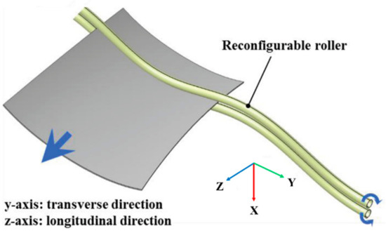
Figure 1.
Schematic illustration of the flexibly-reconfigurable roll forming (FRRF) process.
2. Experiment
2.1. FRRF Equipment
The FRRF technique forms the desired shape of a surface by adjusting the strain in the sheet metal blank. In other words, the curvature is formed from the strain variations in the thickness direction of the sheet. In this experiment, two rollers were used for this purpose, and the FRRF equipment was arranged around these rollers. The position of each roller was determined by the target curvature radius in the transverse direction, the compressive strain difference between the center and tip of the blank, and the width (length in the transverse direction) of the original blank. The basic position of each roller was first set based on the target curvature of the blank, in its transverse direction. The final position of each roller was then calculated based on the compressive strain. The FRRF equipment was designed in previous studies [16,17], and this machine consisted of numerous forming roller modules, a curvature guide assembly, a guide-height-adjusting module, and a transmitter. The complete configuration of the equipment is shown in Figure 2. The curvature guide assembly adjusted the height of the guide, which controlled the upper and lower roller curvature by means of a servo motor. Forming roller modules rotated the corresponding rollers when the blank was placed between the upper and lower rollers by the means of the motor. The guide-height-adjusting module moved the roller guide to set the curvature of the roller. Ideally, the number of guide-height-adjusting modules should be equal to the number of guides, however, due to cost restraints, the combination of a single transmitter and only one servo motor was utilized in this experiment. The servo motor was moved to each roller guide height by means of a linear guide. The height was calculated according to the input value specified by the user, and the servo motor controlled the height of the roller guide as a calculated position. Figure 3 shows a picture of the actual FRRF equipment used. All experiments were performed using this machine.
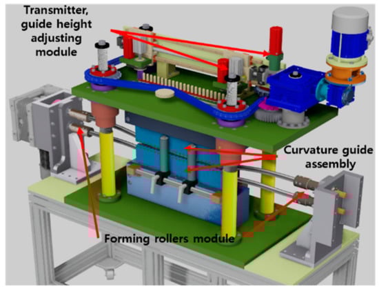
Figure 2.
Configuration of the entire equipment.
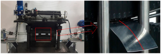
Figure 3.
FRRF apparatus.
2.2. Experiment Conditions
To determine the number of samples necessary for the regression analysis, both dependent and independent variables were selected. The dependent variable in this study is the curvature radius in the longitudinal direction from the FRRF experimental results, and the independent variables are the maximum compression value, the transverse curvature radius, and the width of the initial blank. By combining these three independent variables, the curvature radius in the longitudinal direction (dependent variable) was determined. To obtain an appropriate number of samples, a design of experiments was undertaken, exploiting a three-level, three-factor full factorial design.
The deformation prediction of the target surface was the main focus of this study, and this deformation shape determined by the position of the flexible roller. The position of the roller can be defined by the compression value of each roller, the blank’s curvature radius in the transverse direction and the width of the blank. The above three variables are controllable elements in the FRRF technology and they are more correlatable with the dependent variables than other variables. Therefore, these three parameters were selected as the independent variables that influence the dependent variable. The minimum compression applied to the blank was set at 0%; thus, the maximum compression value was selected as an independent variable. In this research, the target surfaces were convex and saddle-type surfaces, the most frequent double-curvature surfaces in the industry. To form a convex-type surface in the FRRF process, the compression value at the central position of the blank must be larger than that of the edge-line portion. Conversely, to form a saddle-type surface in the FRRF process, the compression value of the central position of the blank must not be larger than that of the edge-line portion. In the case of a convex-type surface, the maximum compression was applied at the center line. In the case of a saddle-type surface, the maximum compression was applied at the edge line. Generally, the compressive strain was limited to 10% of the initial blank thickness, owing to the extreme difficulty of achieving higher strains. In addition, a much smaller compressive strain would not form the curvature. Thus, the minimum compressive strain was determined as 2%. The compressive strain parameters were selected at 2%, 6%, and 10% of the initial blank thickness. The minimum transverse radius of curvature that the equipment can operate at is 1000 mm. Therefore, a radius of up to twice the minimum radius of curvature was selected as a boundary condition. The magnitude of this independent variable was selected as 1000 mm, 1500 mm, and 2000 mm. The level of the remaining independent variable (the width of the initial blank) was selected as 100 mm, 125 mm, and 150 mm. The size of the blank was selected within this range for the convenience of the experiment. Table 1 summarizes the selected independent variable levels.

Table 1.
Levels of the design variables.
The sheet material used for the FRRF experiment was made of Al 5052-H32 with an initial thickness of 1 mm. The physical properties of the material were as follows: Young’s modulus of 70.3 GPa, Poisson’s ratio of 0.33, and density of 2.68 g/cm3. In order to confirm the material properties for this sheet in the plastic region, the stress–strain curve was obtained using a dynamic tensile test machine (Instron). The resulting stress–strain curve is shown in Figure 4, and the yield strength and tensile strength are confirmed from this graph. The yield strength of the material was 176 MPa and the tensile strength was 260 MPa. Table 2 summarizes the physical properties of this sheet material.
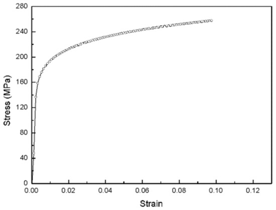
Figure 4.
Stress–strain curve of Al 5052-H32.
Table 2.
Material properties of Al 5052-H32.
3. Experimental Results and Regression Model
3.1. Experimental Results
FRRF experiments were conducted based on the conditions described in the previous section. The target surfaces were convex and saddle-type curved surfaces of various curvature radiuses, and the experiments were conducted with consideration to each parameter. Figure 5 shows the FRRF experimental results. Figure 5a shows the convex-type results, and Figure 5b shows the saddle-type results. Since the sample data in this study consisted of curvature values in the longitudinal-direction, surface data was extracted from the resulting samples using a 3D scanner. In the surface data, the center-line curvature profile of the formed sheet was used, and the radius of curvature was measured with respect to three points, i.e., the start point, center point, and end point.
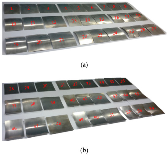
Figure 5.
Results of the experiment using the FRRF apparatus. (a) Convex shape and (b) saddle shape.
From the experimental results, the trends with respect to each parameter could be analyzed. Firstly, in terms of the maximum compression value, the largest and smallest radii of curvature appeared for an initial blank thickness of 2% and 10%, respectively. Naturally, the greater the compression, the smaller the radius of curvature. Secondly, the experimental results confirmed that the larger the transverse radius of curvature, the greater the radius of curvature in the longitudinal direction. Finally, with respect to the width of the blank, opposite tendencies were observed in the case of convex- and saddle-type surfaces. In the convex-shaped samples, the radius of curvature increased as the width of the blank increased, but the opposite trend was observed for the saddle-shaped samples. The measured data for the convex and saddle shapes are given in Table 3 and Table 4, respectively. The summarized results were used as sample data for the regression analysis.
Table 3.
Statistical table for convex shape.
Table 4.
Statistical table for saddle shape.
3.2. Regression Analysis Model
As defined earlier, the independent variables that affect the experimental results include the maximum compression value, transverse radius of curvature, and the width of the initial blank. The first step in the regression analysis is determining a suitable regression model. To achieve this, the main influence of the independent variables and their interactions must be confirmed. The investigation of the influence and interactions was conducted using MATLAB. Figure 6 shows the main effect of each dependent variable, where X1 is the maximum compression value, X2 is the radius of curvature of the original blank in the transverse direction, and X3 is the width of the original blank. All design variables demonstrated mildly quadratic behavior on the dependent variable. Figure 7 shows the interactions among the design variables. Differences can be observed among the slopes of the interaction graphs, indicating different degrees of interaction among the design variables. The regression model selected considering these points is summarized in Equation (1):
where is the radius of curvature in the longitudinal direction (dependent variable), is the maximum compression value (independent variable 1), is the transverse radius of curvature (independent variable 3), is the width of the initial blank (independent variable 2), are the regression coefficients, and is the error value. After selecting the appropriate regression model, the regression coefficients were estimated from the data obtained in the FRRF experiments. Generally, the coefficients can be obtained by the least square method, which was used to calculate the regression coefficients in Equation (1), such that the sum of the error values was minimized. Hence, the function of the least square method can be expressed as in Equation (2), which can be simplified and written in matrix form [18].
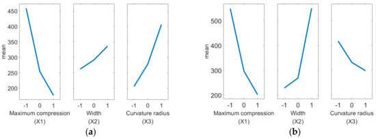
Figure 6.
Plots of the main effects of the design variables. (a) Convex shape and (b) saddle shape.
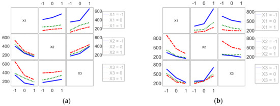
Figure 7.
Plots of the interactions of the design variables. (a) Convex shape and (b) saddle shape.
In this equation, , , , and are defined as follows:
where n is the number of cases and p is the number of independent variables in each interaction. Equation (3) is solved for the regression coefficients as follows:
In the present study, there were 10 unknown coefficients; those estimated using Equation (4) are presented in Table 5 for each respective case.
Table 5.
Estimated regression coefficients.
3.3. Goodness-of-Fit of the Regression Model
To validate the regression model, a goodness-of-fit test was conducted. In the previous study [15], goodness of fit about the regression model was already validated. Thus, the procedure of fit test is carried out in the same way as Ref [15]. Initially, the R-squared value was determined; this value is the yardstick for evaluating the suitability of a regression model developed using the sample data. In other words, the R-squared value is a measure of how well the variability of y is accounted for by the regression variables of a model. The closer the value of R-squared is to 1, the better the regression model fits the data. This value is calculated as follows:
where , , and . SSE is the sum of the squared errors, SST is the total sum of squares, SSR is the regression sum of squares, is the average value of the data, denotes the actual data values, and denotes the estimated data values. The root-mean-square error (RMSE) is an intuitive and reasonably accurate evaluation metric, while the normalized root-mean-square error (NRMSE) is used to evaluate the relative accuracy of the regression model using Equation (6). In contrast to the R-squared value, the NRMSE indicates smaller error as it approaches zero.
In the case of a convex-shape, the R-squared value and NRMSE were calculated to be 0.9724 and 0.0423, respectively, and the corresponding results for the case of the saddle-shape were 0.9273 and 0.0615, respectively. In general, when experimental results are utilized as sample data, an R-squared value greater than 0.8 is considered as being appropriate; the calculated R-squared values achieved here were higher than 0.9. In addition, the NRMSE values were almost zero, suggesting a very high accuracy of the regression model. The regression model can therefore be considered as being appropriate.
For an intuitive comparison, it is also necessary to confirm the difference between sample data and data estimated by the regression model. Figure 8a,b show the graphs of the observed curvature of sample data versus the predicted curvature from the regression model, and Figure 9a,b show the differences between the original samples and the estimated values for the saddle and convex shapes, respectively. The figures demonstrate that the trends of the estimates follow those of the sample experimental data.
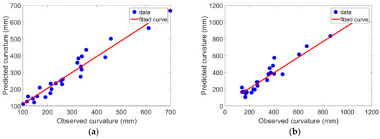
Figure 8.
Graph of observed versus predicted curvature. (a) Convex shape and (b) saddle shape.
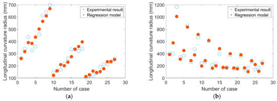
Figure 9.
Difference between the original and estimated data. (a) Convex shape and (b) saddle shape.
To evaluate the accuracy of the estimation model, the percentage errors were investigated. The red circle in Figure 9 is the estimated result, yi, from the regression model, and the percentage error values between the estimated data and the original data are shown in Table 6 together. The maximum and minimum percentage errors for the convex cases were determined to be 29.0% and 0.1%, respectively. Most of the error values for the convex cases were within 18%, and the mean percentage error was 10.7%. Additionally, the corresponding values for the saddle-shaped samples were almost the same. The maximum and minimum percentage errors were 59.0% and 1.6% respectively. As evident, the former value was very high but, even when this was included in the analyses, the mean percentage error resulted in 16.2%, which was lower than the acceptance threshold, indicating that the regression model might still follow the general trend of the FRRF process. The model can therefore be used to predict the resulting output of the process. Figure 10a,b show the residual plots for the convex and saddle shaped samples, respectively. The presence of a definite pattern in the residual plot would suggest that some explanatory variables were missing from the regression model however, there were no definite patterns apparent in the results shown in Figure 10, confirming that no explanatory variables were missing from the obtained regression model. The mean residual values were also examined; for the convex and saddle-shapes, these were calculated to be 2.0527 × 10⁻¹⁴ and 5.7370 × 10⁻¹⁴, respectively. As might be observed, the mean residuals for both cases were therefore nearly zero. The results of the goodness-of-fit tests for both cases are summarized in Table 7.
Table 6.
Estimated results and percent error.
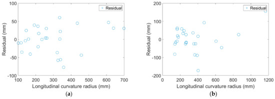
Figure 10.
Plot of residuals. (a) Convex shape and (b) saddle shape.
Table 7.
Summary of results of the goodness of fit tests.
One of the most important assumptions in response surface methodology is that the error has a Gaussian distribution with a zero mean, and this is also assumed in the application of the least square method. It is therefore necessary to confirm the normality of the sample data. Figure 11 shows the data normality plots. In both the saddle and convex-shaped cases, almost all the sample data fits well within a normal distribution. However, two high residual values indicate some discrepancies. A frequency distribution histogram of sample data was used to ascertain the normality of the distributions. Figure 12a,b show the histograms for each case. Both graphs plot bell shapes, denoting the normal distributions of the model results. The curve in Figure 12a has a narrow bell shape because the residual values in the convex case were all small. Compared to Figure 12a, Figure 12b shows a bell shape with a long tail, which means that the error distribution for the saddle-shaped case was wider than for the convex-shaped case. Nevertheless, since the plot shows a bell shape, it is taken to follow a normal distribution.
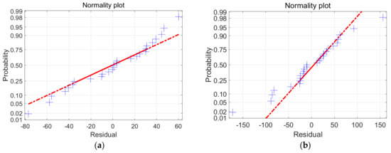
Figure 11.
Normality plot. (a) Convex shape and (b) saddle shape.
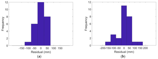
Figure 12.
Histogram of the frequency distribution. (a) Convex shape and (b) saddle shape.
4. Application for Experiment Condition Deduction
4.1. Conversions for a Prediction Model
The desired target shape of the curved surface is the first parameter to be determined in the manufacturing industry, following which, the conditions under which the target surface can be acquired is defined, and later fabrication is carried out to match the condition. Therefore, in order to apply the model to the actual forming process, it was necessary to acquire the experimental conditions for the target surface, by using the prediction model developed in this study. The regression prediction model for the longitudinal curvature of FRRF process can be obtained by using the maximum compression value, the transverse curvature of sheet, and the width of the sheet metal. This model is expressed as an equation with four variables and, if only three variables are determinable, the other may be calculated. Combining the dependent variable with the independent variable X2 (the radius of curvature of the original blank in the transverse direction) determines the shape of target surface, and the independent variable X3 (the width of the original blank) defines the dimension the sheet. Therefore, the desired target surface is determined by these three variables, and the other variable is the forming condition to fabricate that target surface. In other words, the X1 variable could be deduced from input y and X2, whilst X3 deduced according to the target surface shape by the user. In order to deduce the X1 value, the right-hand side of Equation (1) needed to be transposed to the left-hand side. In order for this equation to be true, all sum of terms with appropriate X1 values must be zero. An optimization by means of a numerical analysis was performed to deduce an appropriate value for X1. The univariate method was one of the direct search methods that were used, as it is a simple unconstrained optimization technique whose iterative scheme is shown in Figure 13. The unit of X1 is a percentage, whose values below 0.01 were judged as insignificant. Thus, the step length of this optimization process was considered as 0.01. The convergence condition was also selected so that the residual value of the target surface curvature radius was below 0.5 mm. The assumptions of the FRRF forming conditions were carried out in the following section by utilizing this same optimized technique.
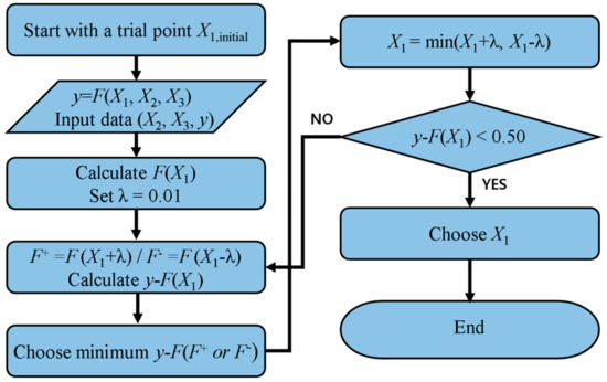
Figure 13.
Iterative scheme of the compression condition deduction using the univariate method.
4.2. Assumptions Underlying the Experimental Characteristics
By using the numerical analysis method described in the section above, the compression characteristics for forming the actual target surface was derived. By utilizing this prediction model, it was possible to confirm the experimental characteristics (compression conditions) suitable for each shape, which was extracted as the target surface. The characteristics of the target surface were randomly acquired from 10 samples (for each of the two forms) by using the Latin-hypercube design; these sampling characteristics are summarized in Table 8 and Table 9. The compression conditions were predicted according to each sampling condition. For the first saddle-shape sample, the maximum compression value to manufacture a target surface, which had a transverse curvature radius of 1405.1036 mm and a longitudinal curvature radius of 498.6408 mm with a width of 102.8773 mm, was deduced as 2.07%. Similarly to the saddle-shape sample, the first convex-type sample required a 2.67% compression value to form the target surface, which had a transverse curvature radius of 1111.9200 mm and a longitudinal curvature radius of 257.9682 mm, with a width of 105.2663 mm. The calculated compression values were applied to the regression model to confirm that the compression values by each condition were in conformance to the results estimated in the previous section. Table 10 and Table 11 show the results of the compression characteristics deduced by numerical analysis based on each sample. In this table, y’ represents the estimated longitudinal curvature radius by using the deduced compression value, and the comparison between regression model results and numerical analysis results are also shown in this table. It has been shown that the difference in the longitudinal curvature radius (|y − y′|) was within 1.0 mm for all samples. In other words, the results suggest that it was possible to utilize the model corresponding to the compression condition derivation for forming the actual target surface, by converting the acquired regression analysis model. Through a comparison with actual experimental results, the reliability of this prediction model was investigated. Using this prediction model, the compression condition for forming a saddle-type target surface with a transverse curvature of 2000 mm, a longitudinal curvature of 266.447 mm, and a sheet material width of 150 mm was calculated to be about 8.96%. From the actual experimental results, the compression value to form the target surface, which had the longitudinal radius of curvature matching the condition, was confirmed as 10%, a result that was not significantly different from the prediction model. Similarly to the saddle-type sample, the predicted compression condition to produce the convex-type target surface with a longitudinal curvature of 255.129 mm, a transverse curvature of 2000 mm, and the width of the sheet material of 150 mm, was calculated to be about 9.81%. The experimental result under the same conditions results in a 10% compression value.
Table 8.
Statistical table for the convex type random sample.
Table 9.
Statistical table for the saddle type random sample.
Table 10.
Deduced results of the compression condition for the convex type.
Table 11.
Deduced results of the compression condition for the saddle type.
5. Conclusions
In this study, a statistical model was developed utilizing a regression analysis to predict the outcome of the FRRF process. To obtain the sample data used for the regression analysis, 54 physical experiments were performed using the FRRF equipment. Based on the sample data, a regression model that could predict the radius of curvature in the longitudinal direction in the FRRF process was suggested, and the results were summarized as follows:
- (1)
- To utilize experimental results in the regression model, a three-level, three-factor full factorial design was used. The experiments were conducted using the FRRF apparatus. The maximum compression value, radius of curvature in the transverse direction, and width of the blank were selected as the input parameters, and the radius of curvature in the longitudinal direction of in the FRRF process was the dependent variable. The radius of curvature values in the longitudinal direction, for the experimental samples, was obtained using a 3D scanner.
- (2)
- Regression analysis was conducted using the experimental results as the sample data. A polynomial, nonlinear regression model was used, and a goodness-of-fit test was conducted to confirm the validity of the model. R-squared values, NRMSE, and residual data were examined. The test results fitted well with the experimental data; thus, the regression model was confirmed to follow the trend of the experimental results.
- (3)
- From the completed regression model, it was concluded that it was possible to predict the results of the FRRF process. The optimization for converting the regression model was carried out to deduce the compression characteristics for forming the target surface. The compression conditions for the actual target surface might also be determined by using the converted regression model. This study thus confirms the feasibility of statistically predicting the curvature produced by the FRRF process. Future progress will focus on further research to evaluate the effects of physical properties on the FRRF process, conducted using different materials.
Author Contributions
J.-W.P.—conceptualization, data curation, formal analysis, investigation, writing—original draft preparation; J.K.—Supervision, Writing—review & editing; B.-S.K.—Funding acquisition, Supervision, Writing—review & editing; Also, all authors were involved in discussion for paper.
Funding
This work was supported by the National Research Foundation of Korea (NRF) grant funded by the Korea government (MSIP) through the Engineering Research Center (No. 2012R1A5A1048294) and (No. NRF-2019R1C1C1005721). Also, this study was financially supported by the 2019 Post-Doc. Development Program of Pusan National University.
Acknowledgments
In this section you can acknowledge any support given which is not covered by the author contribution or funding sections. This may include administrative and technical support, or donations in kind (e.g., materials used for experiments).
Conflicts of Interest
The authors declare no conflict of interest.
References
- Olsen, B.A. Die Forming of Sheet Metal Using Discrete Surfaces. Master’s Thesis, Massachusetts Institute of Technology, Cambridge, MA, USA, 1981. [Google Scholar]
- Zhang, Q.; Wang, Z.; Dean, T. The mechanics of multi-point sandwich forming. Int. J. Mach. Tools Manuf. 2008, 48, 1495–1503. [Google Scholar] [CrossRef]
- Yan, Y.; Wang, H.; Li, Q.; Qian, B.; Mpofu, K. Simulation and experimental verification of flexible roll forming of steel sheets. Int. J. Adv. Manuf. Technol. 2014, 72, 209–220. [Google Scholar] [CrossRef]
- Li, M.; Cai, Z.; Sui, Z.; Yan, Q. Multi-point forming technology for sheet metal. J. Mater. Process. Technol. 2002, 129, 333–338. [Google Scholar] [CrossRef]
- Heo, S.C.; Seo, Y.H.; Park, J.W.; Ku, T.W.; Kim, J.; Kang, B.S. Application of flexible forming process to gull structure forming. J. Mech. Sci. Technol. 2010, 24, 137–140. [Google Scholar] [CrossRef]
- Park, J.W.; Kim, J.; Kim, K.H.; Kang, B.S. Numerical and experimental study of stretching effect on flexible forming technology. Int. J. Adv. Manuf. Technol. 2014, 73, 1273–1280. [Google Scholar] [CrossRef]
- Abebe, M.; Park, J.W.; Kim, J.; Kang, B.S. Numerical verification on formability of metallic alloys for skin structure using multi-point die-less forming. Int. J. Precis. Eng. Manuf. 2017, 18, 263–272. [Google Scholar] [CrossRef]
- Quan, G.Z.; Ku, T.W.; Kang, B.S. Improvement of formability for multi-point bending process of AZ31B sheet material using elastic cushion. Int. J. Precis. Eng. Manuf. 2011, 12, 1023–1030. [Google Scholar] [CrossRef]
- Abebe, M.; Park, J.W.; Kang, B.S. Reliability-based robust process optimization of multi-point dieless forming for product defect reduction. Int. J. Adv. Manuf. Technol. 2017, 89, 1223–1234. [Google Scholar] [CrossRef]
- Yoon, J.S.; Son, S.E.; Song, W.J.; Kim, J.; Kang, B.S. Study on flexibly-reconfigurable roll forming process for multi-curved surface of sheet metal. Int. J. Precis. Eng. Manuf. 2014, 15, 1069–1074. [Google Scholar] [CrossRef]
- Kang, B.S.; Yoon, J.S. Mold-less Pate Forming Apparatus with Flexible Rollers. PCT Patent PCT/KR2013/007642, 27 August 2013. [Google Scholar]
- Liu, P.; Ku, T.W.; Kang, B.S. Shape error prediction and compensation of three-dimensional surface in flexibly-reconfigurable roll forming. J. Mech. Sci. Technol. 2015, 29, 4387–4397. [Google Scholar] [CrossRef]
- Kim, H.H.; Yoon, J.S.; Kim, J.; Kang, B.S. Feasibility Study on Flexibly Reconfigurable Roll Forming Process for Sheet Metal and Its Implementation. Adv. Mech. Eng. 2014, 6, 958925. [Google Scholar]
- Yoon, J.S.; Kim, J.; Kang, B.S. Deformation analysis and shape prediction for sheet forming using flexibly reconfigurable roll forming. J. Mater. Process. Technol. 2016, 233, 192–205. [Google Scholar] [CrossRef]
- Park, J.W.; Yoon, J.; Lee, K.; Kim, J.; Kang, B.S. Rapid prediction of longitudinal curvature obtained by flexibly reconfigurable roll forming using response surface methodology. Int. J. Adv. Manuf. Technol. 2017, 91, 3371–3384. [Google Scholar] [CrossRef]
- Yoon, J.; Park, J.; Son, S.; Kim, H.; Kim, J.; Kang, B. Development of a Flexibly-reconfigurable Roll Forming Apparatus for Curved Surface Forming. Trans. Mater. Process. 2016, 25, 161–168. [Google Scholar] [CrossRef]
- Son, S.; Yoon, J.; Kim, J.; Kang, B. Effect of Shape Design Variables on Flexibly-Reconfigurable Roll Forming of Multi-curved Sheet Metal. Trans. Mater. Process. 2014, 23, 103–109. [Google Scholar] [CrossRef][Green Version]
- Myers, R.H.; Montgomery, D.C.; Anderson-cook, C.M. Response Surface Methodology—Process and Product Optimization Using Designed Experiments, 3rd ed.; John Wiley & Sons: Hoboken, NJ, USA, 2009; pp. 13–62. [Google Scholar]


© 2019 by the authors. Licensee MDPI, Basel, Switzerland. This article is an open access article distributed under the terms and conditions of the Creative Commons Attribution (CC BY) license (http://creativecommons.org/licenses/by/4.0/).