1. Introduction
During the manufacturing of components, various residual stress states may occur in the material because of the process. In the past, there have been several investigations of the relationship between forming parameters such as deformation state or temperature profile and resulting residual stresses by experiments and simulations; see for instance [
1,
2,
3]. The work of [
4] investigated process parameters, deformation state, and temperature time profile with special regard to the spring-back behavior after a hot stamping process. It is noteworthy that the residual stresses resulting from metal-forming processes are generally known to have negative effects, regarding e.g., lifetime, so that avoidance or minimization during the manufacturing process is usually targeted instead of specifically influencing component properties. For example, positive effects on the fatigue life of components due to residual compressive stresses have already been achieved by the surface treatment process of shot peening applied as an additional process step [
5]. The overall objective pursued in this paper is to analyze and adjust hot forming processes to achieve a favorable residual stress profile directly from the forming stage. To achieve defined material properties in the formed component, targeted cooling or heat treatment is necessary [
6]. For example, quenching from the forging temperature is an energy-efficient way of tempering components [
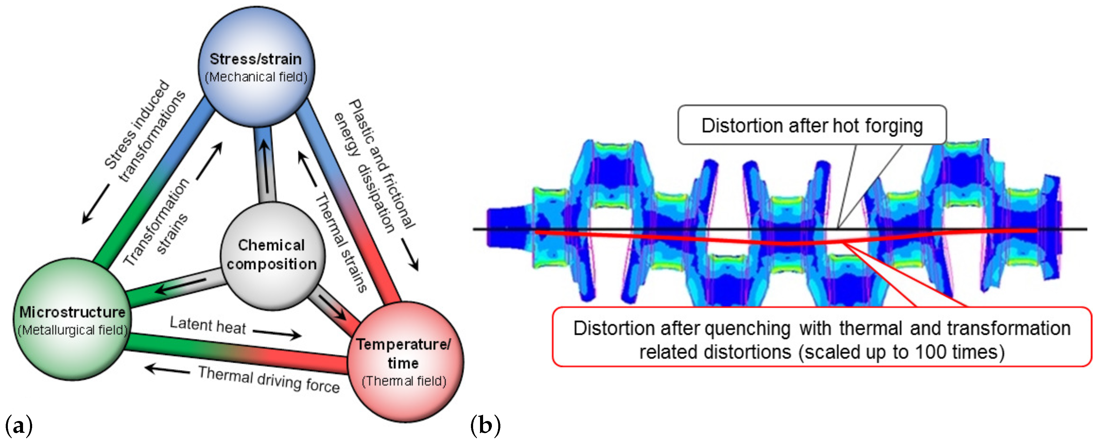
7]. Hot forming as a thermo-mechanically coupled process offers the potential for many adjustment parameters to influence residual stresses. As a consequence, complex material phenomena arising during the individual process steps interact and emphasize each other, decisively affecting the final component properties and making the virtual process design rather complicated, cf.
Figure 1.
In general, according to [
10], there are three different types of residual stresses which are explained in the following. Residual stresses of the first type refer to the complete component and can be defined as macroscopic. The difference between the mean stress of a grain and the macroscopic residual stress is regarded as residual stress of the second type, while the location-dependent deviations of the stresses within the grain from the sum of first and second type are called residual stresses of the third type, cf. [
11,
12,
13].
The resulting mechanical properties of steels strongly depend on the physical processes, e.g., hardening and phase transformations, occurring during the material production and the manufacturing. Thus, in numerical modeling, the consideration of these aspects is crucial to obtain good reliability and prediction.
The diffusionless phase transformation, i.e., austenite to martensite, is a key aspect in the improvement of metal properties. In [
14], as well as [
15], macroscopic constitutive models for its consideration in a large strain plasticity setting is proposed. In the investigations carried out by [
16,
17], a macroscopic approach to simulate the aforementioned transformation process as well as the effect of transformation induced plasticity (TRIP) is introduced. In their research [
8,
18] are contributing to the Finite Element (FE) supported calculation of phase transformations regarding the anisotropic transformation strains during martensitic transformation by using a user-defined FE code based on the mathematical network of [
19,
20]. In general, for fully coupled thermo-mechanical-metallurgical process simulations on the macroscale following [
21,
22], FE codes based on the theory of additive strain decomposition (ASD) are used. The total strain increment is decomposed into an elastic-, plastic-, thermal-, transformation- and a TRIP-strain component, respectively. In the work of [
16], first steps towards a multiscale approach within a homogenization scheme are presented.
Based on these investigations in [
23,
24], the multiscale approach is extended to further phases, e.g., bainite, pearlite, and steel types, e.g., low alloy ones. All the previously mentioned works use the FE Method for the numerical simulation. A further technique for the description of the physical aspects is the Multi-Phase-Field (MPF) model, which is introduced in [
25,
26,
27]. This model is based on the consistent formulation of diffusional and surface driven phase transitions and allows the calculation of interfacial tension, multiphase thermodynamics and elastic stress balance in multiple junctions between an arbitrary number of grains and phases. Numerous publications have picked up on this model for the description of a variety of multi-physics effects, starting from single grain simulation up to the evolution of dendrites. In context of this publication, it is referred to [
28,
29,
30], wherein the transformation process inside metals during production and manufacturing are taken into account. An implementation of the MPF model is available in the software library OpenPhase, which is distributed under the GNU General Public License (GPL) and is free of charge; see [
31]. Actual studies concerning martensite transformation using the phase-field theory can be found in [
32,
33,
34,
35].
In the scope of this work, an insight into the experimental and numerical analysis of the material behavior in thermo-mechanical forming processes as well as simulation approaches of residual stresses on different scales is provided. The paper is organized as follows:
Section 2 describes the experimental treatment of the forming process of cylindrical specimen. The macroscopic FE simulation model is presented in
Section 3. In
Section 4, the macroscopic results of the experiment and the simulation are compared. A numerical process of the investigation of residual stresses on mesoscale and microscale is described in
Section 5.
Section 6 provides a conclusion.
2. Experimental Procedure
To investigate the development of residual stresses, the steel alloy 1.3505 (DIN designation according to [
36]: 100Cr6) was thermo-mechanically processed by upsetting at
with subsequent cooling. Following [
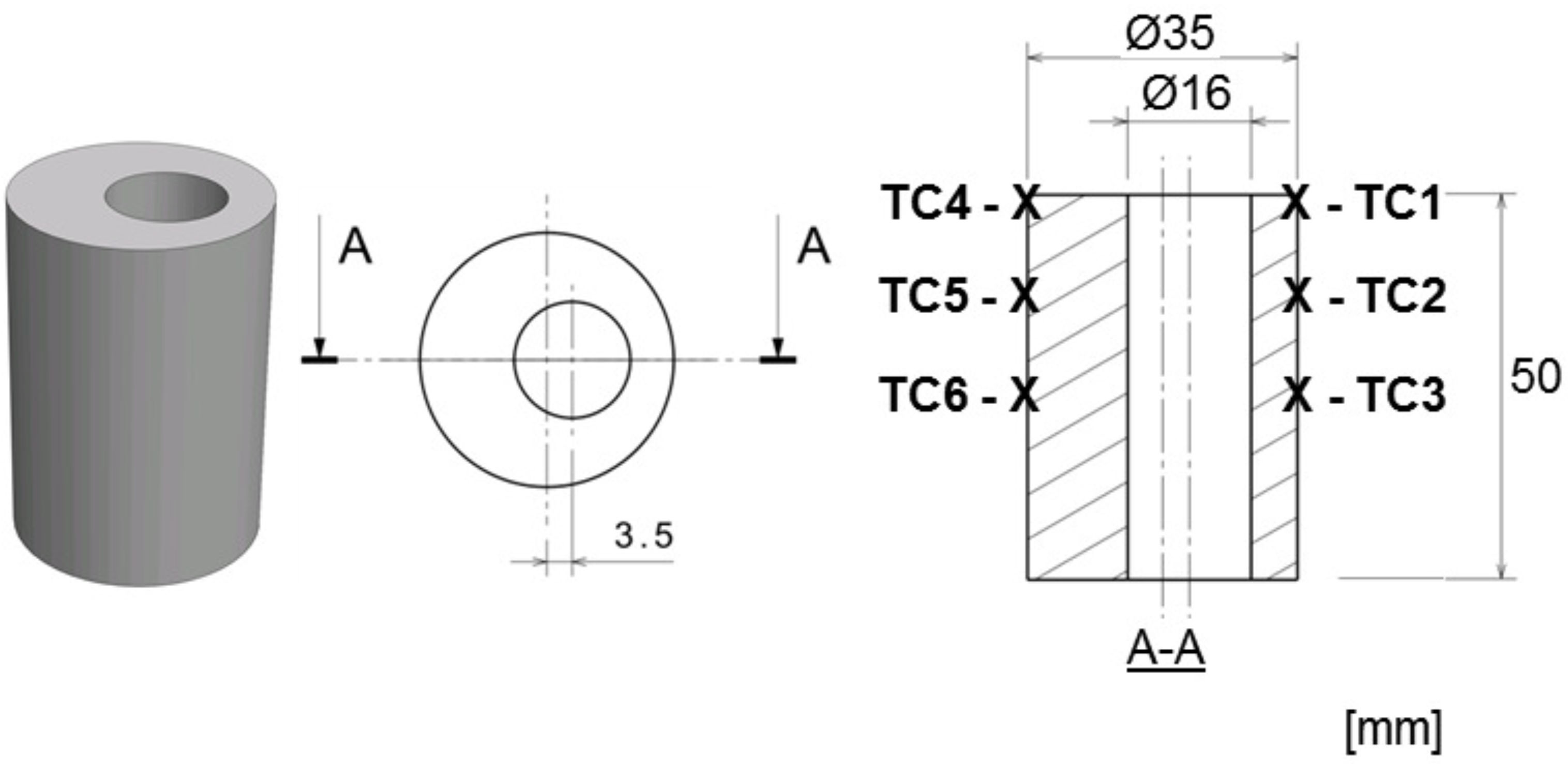
20], cylindrical specimen with eccentric holes were used, as inhomogeneous residual stresses are expected over the circumference of the specimen. The specimen were prepared with six thermocouples as shown in
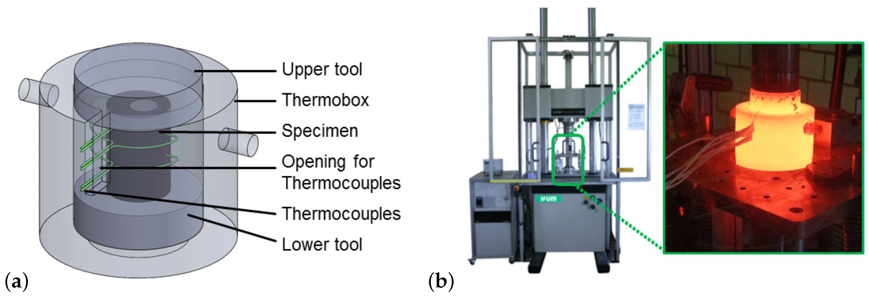
Figure 2. Three thermocouples are located on the thin-walled side (positions are indicated as TC1 to TC3) and three thermocouples on the thick-walled side (TC4 to TC6), respectively. The prepared specimens were placed in a thermobox together with the tools as shown in
Figure 3a which enables the upsetting test to be carried out isothermally.
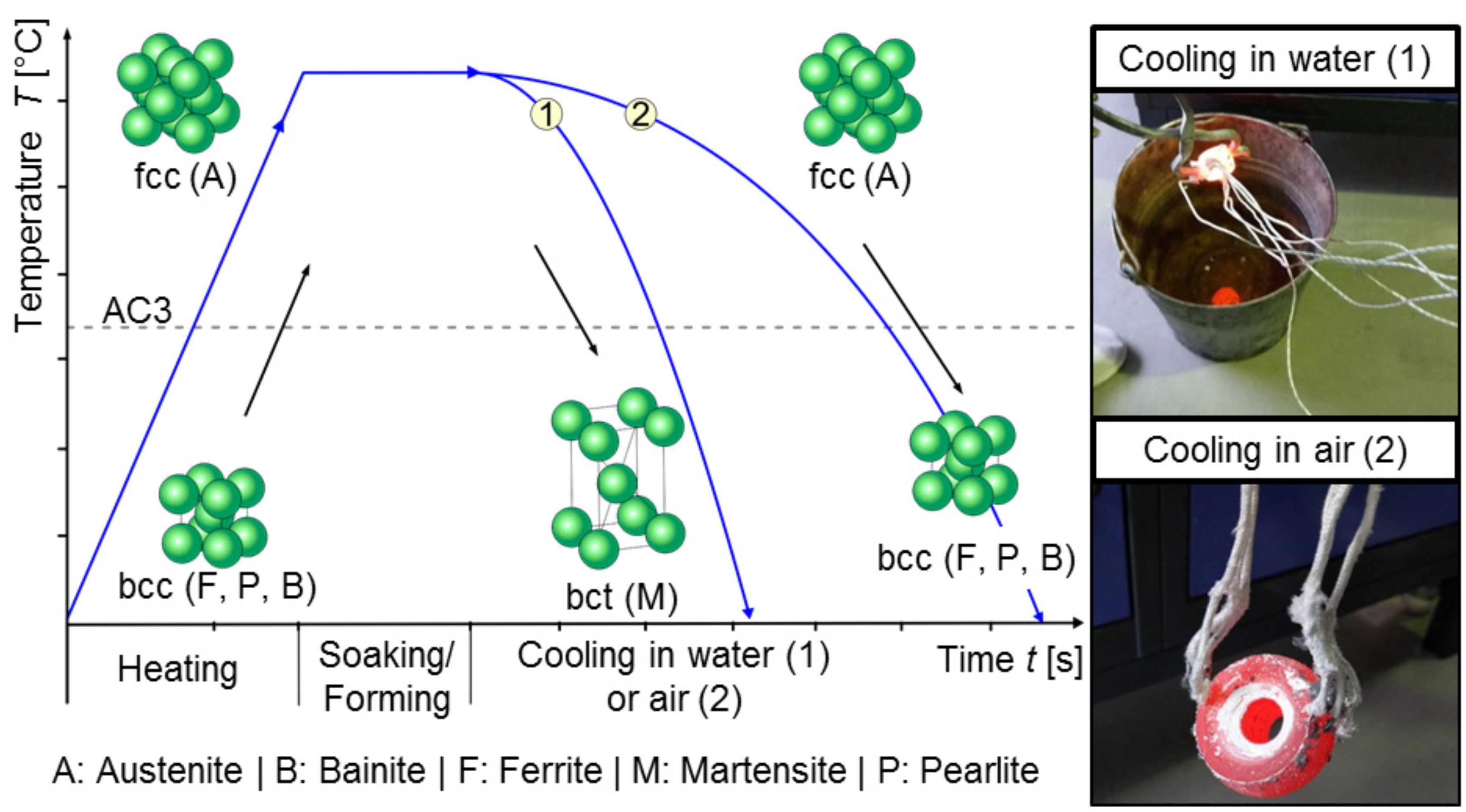
The temperature time profile is shown schematically in
Figure 4, illustrating the process procedure. The prepared specimens were heated to
inside the thermobox including the upper and lower tools in an oven, which has been manufactured by Nabertherm GmbH. After the desired temperature of
had been reached, a ten-minute holding time followed to achieve a homogeneous austenitic structure. Since the austenitization conditions have an influence on the grain size and the grain size in turn has an impact on the phase-transformation behavior, all experiments were carried out using the identical austenitization conditions (
, 10 min), which result in a grain with the ASTM grain size number 8 according to [
37,
38]. Subsequently, the thermobox including the tools and the specimen was transferred to the servohydraulic forming simulator. The specimens were upset from initial height of
to a final height of about
at a punch speed of
. In the next step, the specimen were removed from the thermobox and either quenched in cold water or cooled down to room temperature in still air. During the entire process chain, the temperature was measured via the thermocouples of type K (NiCr-Ni, manufacturer Günther GmbH). The bare thermocouple wires with a diameter of
have been welded directly onto the specimen. Using the measuring amplifier MX1609 (max.
, manufacturer HBM GmbH), the temperatures have been successfully recorded at a sampling rate of
for quenching in water and
for air cooling.
Due to the two cooling media of water and air, different temperature time profiles and consequently different transformation kinematics (see
Figure 4) have been observed in the steel alloys. During rapid cooling in water, a diffusionless transformation occurs, where austenite is transformed into the martensitic body-centered tetragonal (bct) lattice structure. When cooled by air, a body-centered cubic (bcc) lattice with a ferritic, pearlitic, or bainitic microstructure depending on the cooling path is formed, as a consequence of a diffusion-controlled transformation. As a result, various residual stress conditions and distortions are expected in the differently cooled specimen.
After thermo-mechanical processing, both axial and tangential residual stresses were measured on the surface of the specimen at the mid-height. The surface of the specimen at the locus of the measuring point was electrolytically polished, in order to avoid the influence of scale layers on the measurement. Residual stresses were determined by X-ray diffraction employing the
method in accordance with the corresponding DIN norm [
39]. For this purpose a
-diffractometer type XSTRESS X3000 G2 from Stresstech GmbH using
radiation was applied. The measuring spot was determined by a
point collimator, whereas the tilting area of
was varied with a total of nine tilt positions. The evaluation of the residual stress measurements was carried out with the software XTronic (Stresstech GmbH). The X-ray elasticity constants (
,
) and the reference values for the unstressed material (
,
) were taken from the tabular data collection of [
40]. These data of X-ray elasticity constants were calculated as mean values from the so-called Voigt [
41] and Reuß [
42] approaches for the pure alpha iron lattice.
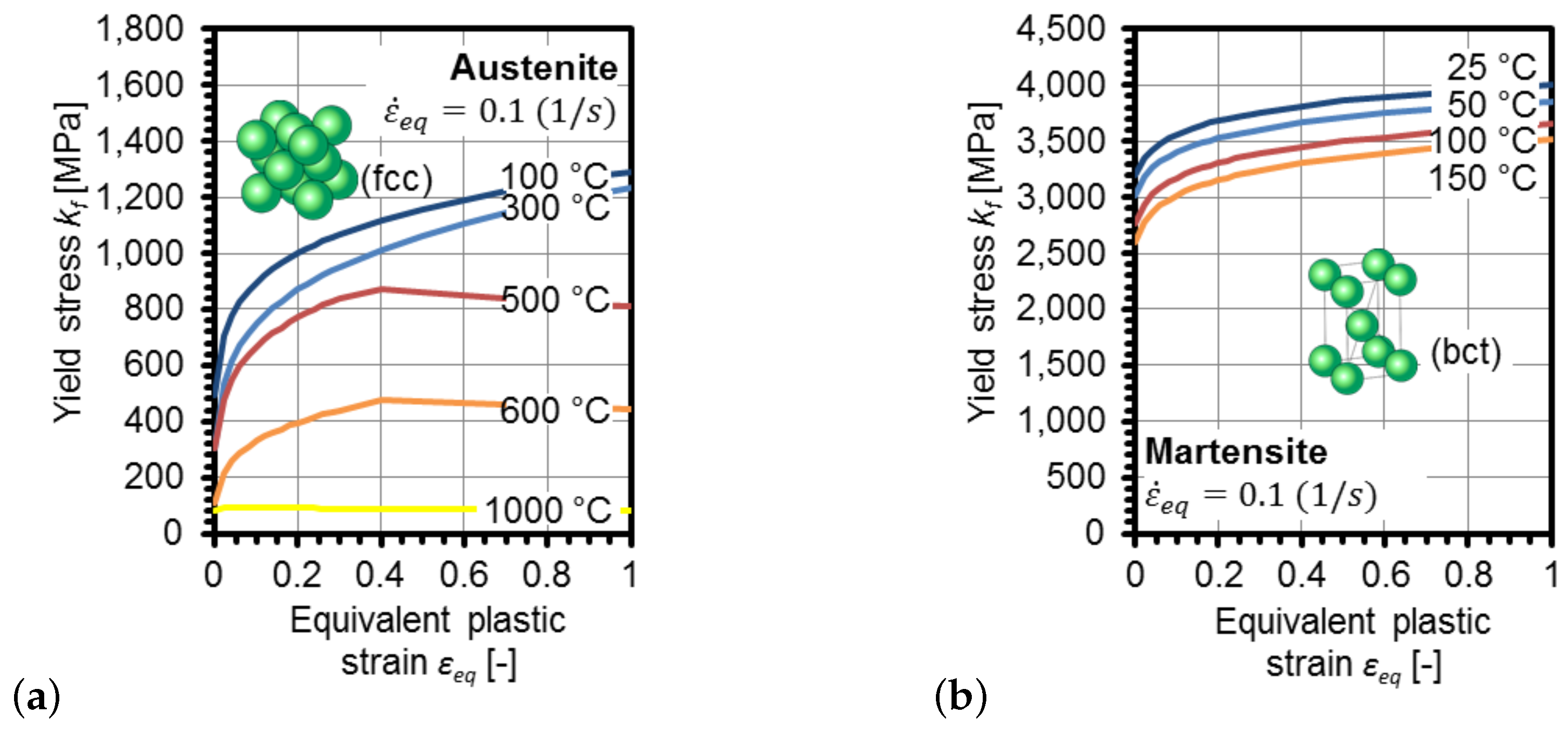
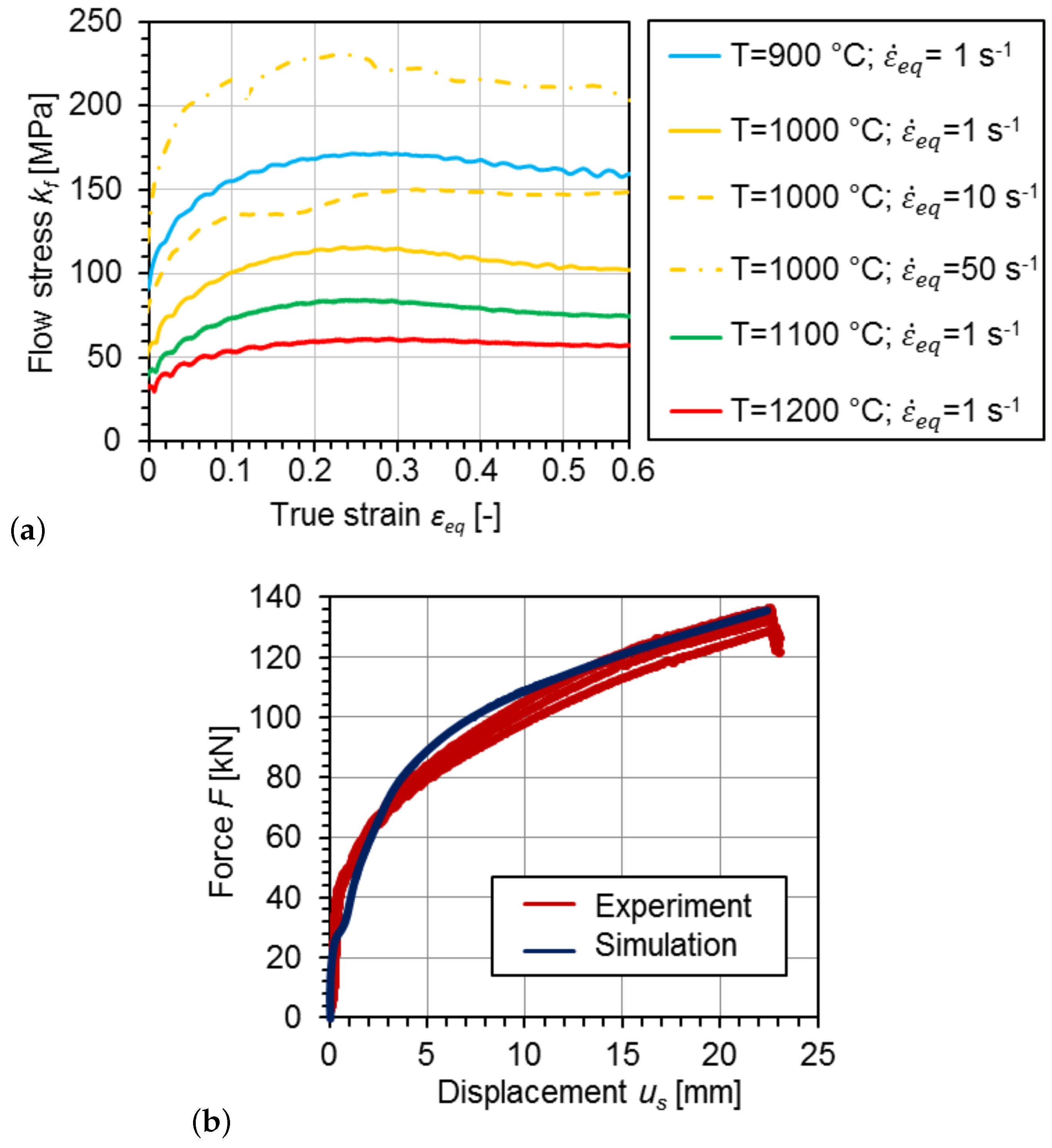
Furthermore, flow curves for the 1.3505 steel alloy were determined by means of standard cylindrical upsetting tests, in order to characterize the flow behavior in the hot forming process. The characterization tests were carried out on the servohydraulic forming simulator Gleeble 3800-GTC at IFUM for the relevant temperatures , , and with the equivalent plastic strain rate . In addition, the tests were carried out at a temperature of with the equivalent plastic strain rates and . Temperature control by means of thermocouples allowed the test to be carried out isothermally.
4. Comparison of Experimental and Numerical Results for Macroscopic Model Validation
The determined flow curves at the investigated temperatures and equivalent plastic strain rates are shown in
Figure 7a. The parameters (
A,
,
,
,
) of the following approach according to [
49], cf. Equation (
1) and
Table 2, were determined using the method of the smallest error squares to continuously describe the flow stress
as a function of equivalent plastic strain
, equivalent plastic strain rate
and temperature
T,
As shown in
Figure 7b, the plasticity model for the hot forming process step was validated by force-displacement-curves from experiment and simulation. The temperature time profiles are subject to several influencing parameters. Simufact.forming therefore considers thermal data, such as specific heat capacity, heat conduction, and latent heat, which were calculated with JMatPro; see
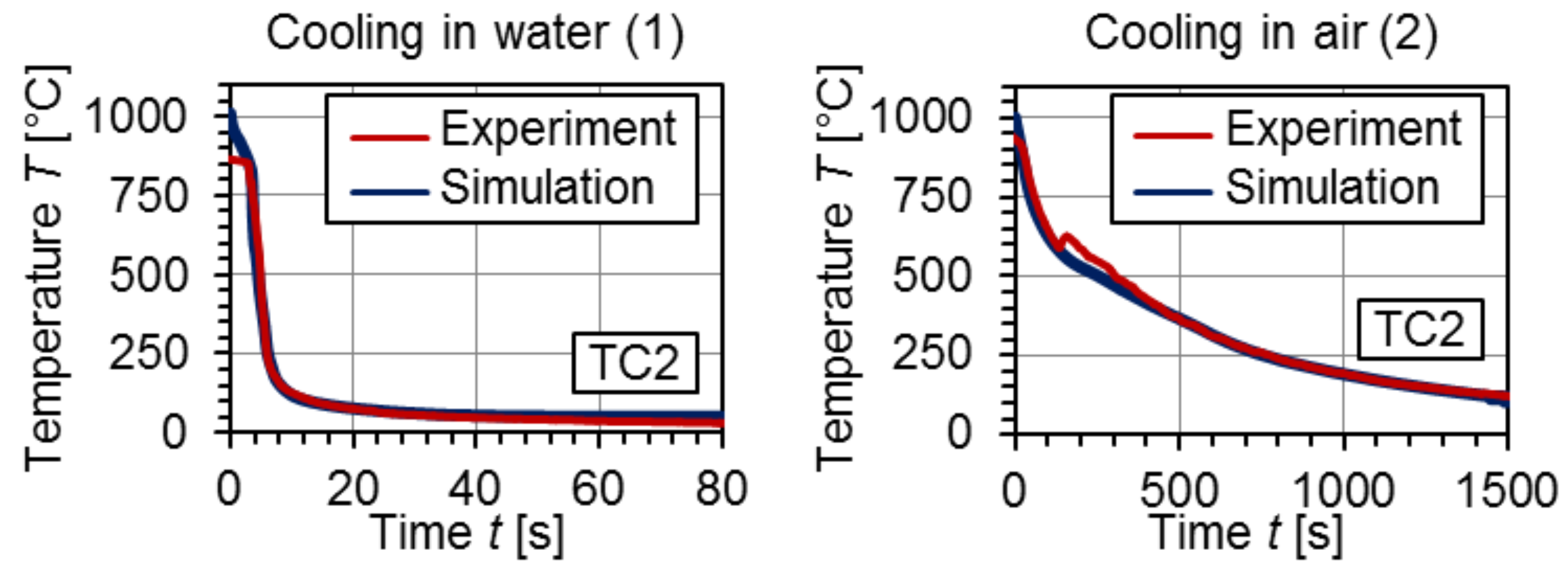
Appendix A. Since the modeling of the correct temperature profile is particularly important for the simulation of the phase transformations and finally the residual stresses, heat transfer coefficients (HTC) were also optimized. The HTC between steel and the cooling media air or water were determined in iterative numerical optimizations to accurately represent the cooling of the specimen in the simulation. Thus, they can be regarded as empirically fitted for the experiment under consideration. Initial values for temperature-dependent HTC for air and water were calculated based on literature data [
50]. In an iterative optimization procedure, the HTCs were adjusted using the experimental data from thermocouple 3 (TC). The calculated HTC values are presented in
Table 3. Afterwards, the temperature profiles of the different measuring points from experiment and simulation, based on the calculated HTC data, were compared. As shown exemplarily for TC 2 in
Figure 8, the temperature profiles could be successfully simulated.
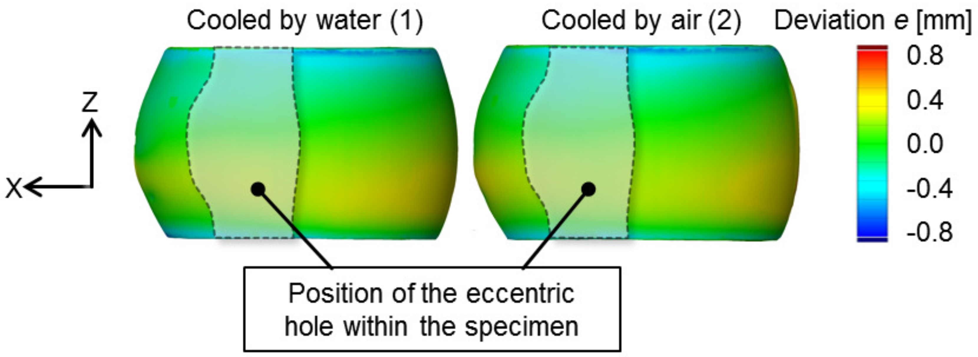
The upset specimen from experiment were optically investigated to evaluate the resulting distortions from thermo-mechanical processing. The CAD-model of a specimen from experiment could be created by 3D scanning, applying the optical measurement system ATOS (GOM GmbH). Subsequently, the dimensional accuracy of the FE simulation was visualized using the software INSPECT (GOM GmbH).
Figure 9 shows the geometry of the specimen from experiment. The contour plot of the deviation
e on this surface indicates the three-dimensional distance in perpendicular direction to the surface of the geometry from the simulation.
A deviation of
shows a perfect match between the geometry from the simulation and the experiment. The algebraic sign of the deviation value indicates if the corresponding area of the geometry from the simulation lies outside (positive sign) or inside (negative sign) the workpiece shape from the experiment. As can be seen in
Figure 9, a maximum deviation of about
was determined.
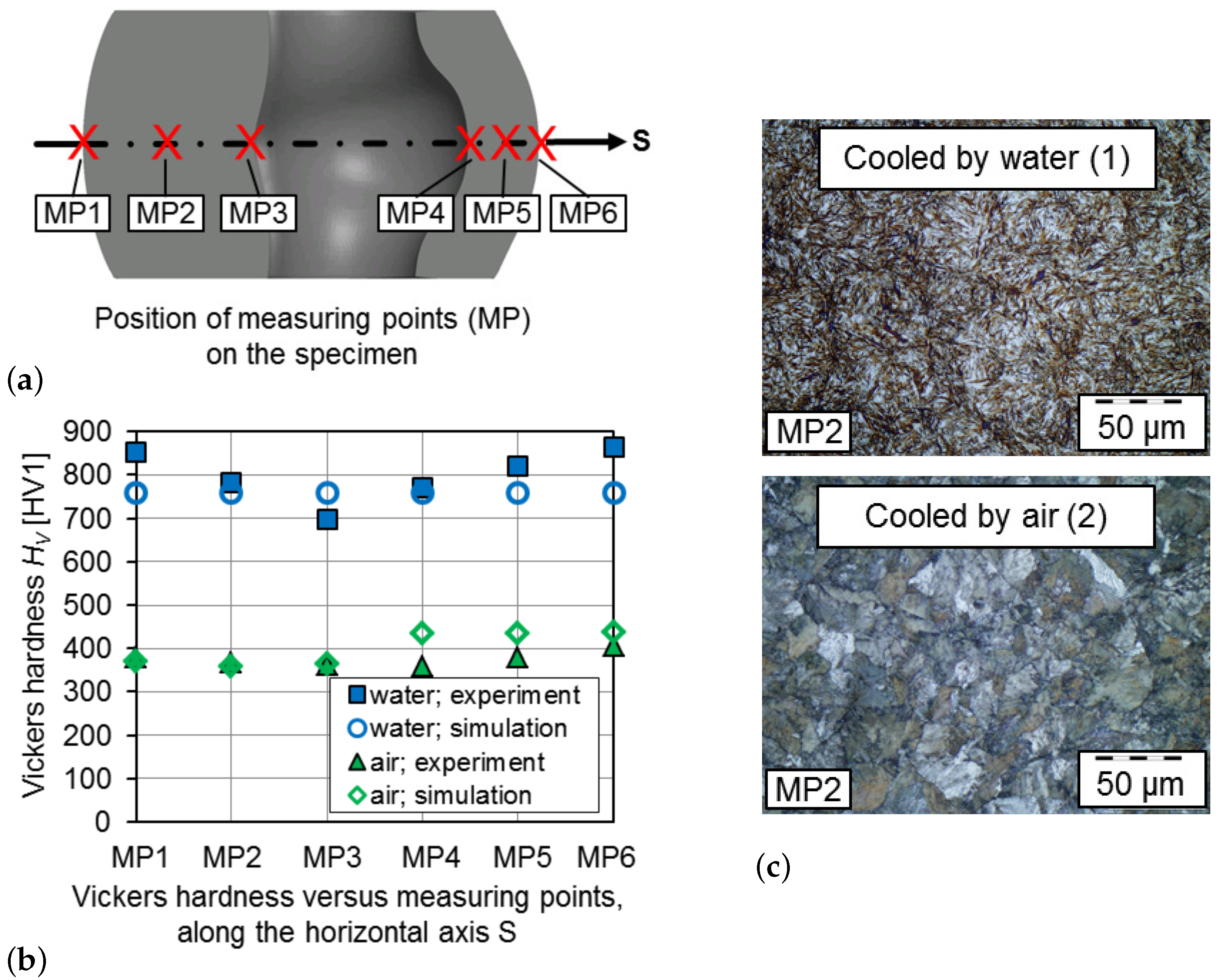
The hardness of the material depends on the resulting phase structure which is related to the transformation mechanisms and the cooling time. Hence, the hardness measurement according to Vickers [
51] provides an important reference point for assessing the quality of the microstructure transformation simulation. For these metallographic investigations, the specimen were cut into two parts by wire erosion as shown in
Figure 10a. Afterwards, Vickers hardness measurements were carried out at six measuring points (MP1 to MP6). The comparison of hardness values from experiment and simulation shows that the evolution of microstructure during cooling could be predicted well by the numerical model, c.f.
Figure 10b. In addition, the corresponding microstructure in MP2 of the differently treated specimen is shown exemplarily in
Figure 10c. As expected, a martensitic structure was formed by cooling in water, recognizable by the needle-shaped structure. A fine striped pearlitic structure was found on the specimen cooled by air, respectively. Consequently, the higher hardness values on the martensitic specimen after cooling in water and the lower hardness values on the pearlitic specimen after cooling in air are plausible.
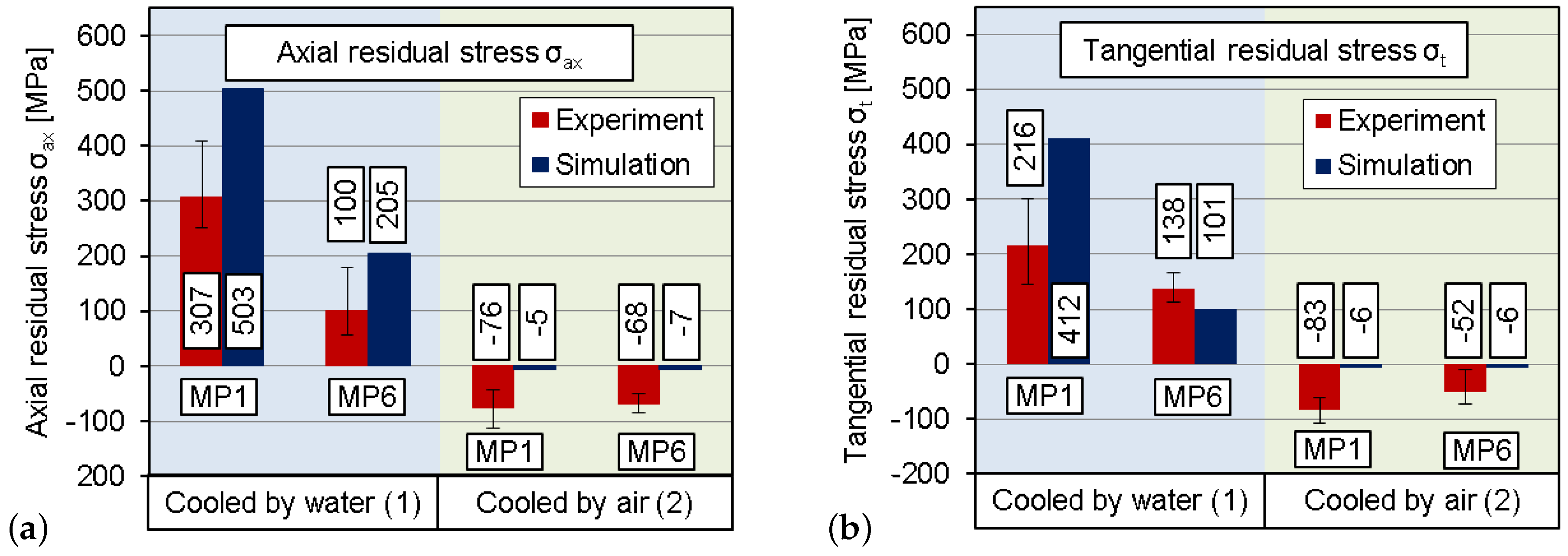
Figure 11 presents a comparison of simulation results with XRD residual stress measurements. Here, the arithmetic mean with the absolute deviations of the tangential
as well as the axial
residual stresses on the specimen surface at the locations of MP1 and MP6 on the mid-height are considered. In the X-ray measurements, negative stresses between
and
were detected on the specimen cooled by air. The simulation also predicts low residual stress values in the range of
to
for this cooling route. These minor residual stresses can be attributed to the diffusion-controlled phase transformation during cooling in air. For the specimen cooled by water, different values were measured on the surface of the thick-walled specimen side (MP1) and the thin-walled specimen side (MP6). The axial residual stress at MP1 is
and at MP6
respectively. In the tangential direction, residual stresses of
at MP1 and
at MP6 were measured. As expected, the geometry of the specimen with an eccentric hole causes an inhomogeneous residual stress distribution.
The developed FE model was able to predict the occurrence of tension or compression stresses for all the considered cases. In addition, the qualitative amount, especially the differences of the residual stresses between MP1 and MP6, could be predicted. However, the simulation overestimates the axial residual stresses at MP1 and MP6 as well as the tangential residual stress at MP1. The tangential residual stress at MP6 could be predicted with a good accuracy.
As shown in
Figure 1, thermal, metallurgical and mechanical interactions in the material must be taken into account for the numerical description of the residual stresses. Due to these numerous interacting parameters, an exact calculation of the residual stresses is challenging. In particular, the TRIP strains take a significant impact on the resulting residual stresses [
8]. Therefore, the calculation of TRIP strains used in the simulation model by MSC.Marc solver could be extended. On the one hand, the load-dependent and reversible back-stress effects resulting from a stress relief during martensitic transformation can be included in the simulations. On the other hand, the work in [
18] shows that the TRIP behavior has different effects on the deformation at tensile and compressive loads. For a further improvement of the model, these influences could be considered separately. With the simulation model presented in this paper, it was possible to make an appropriate qualitative prediction of the macroscopic residual stresses resulting from different cooling routes.
However, it is assumed that local stress gradients have also been developed, for example due to dislocations within the grains resulting from plastic deformations or phase transformations at the microstructural scale. These local deviations represented by residual stresses of second and third type can have a particular influence on the macroscopic stresses. Therefore, in future work in-depth numerical investigations on the microscale are to be performed in order to further analyze the interactions of the residual stresses of first, second, and third type and to quantitatively improve the prediction accuracy of the residual stresses; see
Section 5.
Author Contributions
Conceptualization, funding acquisition as well as supervision of this research project was done by B.-A.B., J.S. and D.B.; The experimental investigations as well as the numerical FE-analyses on the macroscale were carried out by C.K. with the support of A.C.; S.U. adopted the Multi-Phase-Field model based on work of M.S. and R.N. and performed the numerical simulations with help of L.S. and D.B.; C.K. and S.U. took the lead in writing the manuscript; All authors provided critical feedback and helped shape the research, analysis and manuscript.
Funding
Funded by the Deutsche Forschungsgemeinschaft (DFG, German Research Foundation)—374871564 (BE 1691/223-1, BR 5278/3-1, SCHR 570/33-1) within the priority program SPP 2013.
Acknowledgments
The authors thank Ingo Steinbach and Oleg Shchyglo from ICAMS (Interdisciplinary Center for Advanced Materials Simulation) at the Ruhr-Universität Bochum for their scientific support.
Conflicts of Interest
The authors declare no conflict of interest.
References
- Tekkaya, A.E.; Gerhardt, J.; Burgdorf, M. Residual Stresses in Cold-Formed Workpieces. Manuf. Technol. 1985, 34, 225–230. [Google Scholar] [CrossRef]
- Mungi, M.P.; Rasane, S.D.; Dixit, P.M. Residual stresses in cold axisymmetric forging. J. Mater. Process. Technol. 2003, 142, 256–266. [Google Scholar] [CrossRef]
- Von Mirbach, D. Hole-drolling method for residual stress measurement-consideration of elastic-plastic material properties. Mater. Sci. Forum 2014, 768–769, 174–181. [Google Scholar]
- Behrens, B.A.; Schrödter, J. Numerical Simulation of Phase Transformation during the Hot Stamping Process. In Proceedings of the 5th International Conference on Thermal Process Modeling and Computer Simulation, Orlando, FL, USA, 16–18 June 2014; pp. 179–190. [Google Scholar]
- Torres, M.A.S.; Voorwald, H.J.C. An evaluation of shot peening, residual stress and stress relaxation on the fatigue life of ASIS 4340 steel. Int. J. Fatigue 2002, 24, 877–886. [Google Scholar] [CrossRef]
- Seidel, W. Werkstofftechnik—Werkstoffe, Eigenspannungen, Prüfung, Anwendungen, 7th ed.; Hanser: New York, NY, USA, 2007. [Google Scholar]
- Behrens, B.A.; Bleck, W.; Bach, F.W.; Brinksmeier, E.; Fritsching, U.; Liewald, M.; Zoch, H.W. Resource-efficient process chains for high performance parts. Key Eng. Mater. 2012, 504–506, 151–156. [Google Scholar] [CrossRef]
- Behrens, B.A.; Bouguecha, A.; Bonk, C.; Chugreev, A. Numerical and experimental investigations of the anisotropic transformation strains during martensitic transformation in a low alloy Cr-Mo steel 42CrMo4. Procedia Eng. 2017, 207, 1815–1820. [Google Scholar] [CrossRef]
- Courtesy of DKK Co. 2018. Available online: https://www.denkikogyo.co.jp/en/business/hf/technology/simulation2.html (accessed on 1 August 2018).
- Macherauch, E.; Wohlfahrt, H.; Wolfstied, U. Zur zweckmäßigen Definition von Eigenspannungen. Härterei-Technische Mittelungen Z. Für Werkst. Wärmebehandlung, Fert. 1973, 28, 201–211. [Google Scholar]
- Withers, P.J.; Bhadeshia, H.K.D.H. Residual Stress Part 1—Measurement Techniques. Mater. Sci. Technol. 2001, 17, 355–365. [Google Scholar] [CrossRef]
- Withers, P.J.; Bhadeshia, H.K.D.H. Resdiual Stress Part 2—Nature and Origins. Mater. Sci. Technol. 2001, 17, 366–375. [Google Scholar] [CrossRef]
- Bhadeshia, H.K.D.H. Handbook of Resdiual Stress and Deformation og Steel; Chapter Material Factors; The Materials Information Society: Materials Park, OH, USA, 2002; pp. 3–10. [Google Scholar]
- Hallberg, H.; Håkansson, P.; Ristinmaa, M. A constitutive model for the formation of martensite in austenitic steels under large strain plasticity. Int. J. Plast. 2007, 23, 1213–1239. [Google Scholar] [CrossRef]
- Behrens, B.A.; Olle, P. Consideration of phase transformations in numerical simulation of press hardening. Steel Res. Int. 2007, 78, 784–790. [Google Scholar] [CrossRef]
- Mahnken, R.; Schneidt, A.; Antretter, T. Macro modelling and homogenization for transformation induced plasticity of a low-alloy steel. Int. J. Plast. 2009, 25, 183–204. [Google Scholar] [CrossRef]
- Behrens, B.A.; Olle, P.; Schäffner, C. Process Simulation of Hot Stamping in Consideration of Transformation-Induced Stresses; Numisheet: Melbourne, Australia, 2008; pp. 557–562. [Google Scholar]
- Behrens, B.A.; Chugreev, A.; Chugreeva, A. FE-simulation of hot forging with an integrated heat treatment with the objective of residual stress prediction. In Proceedings of the 21st International ESAFORM Conference on Material Forming, Palermo, Italy, 23–25 April 2018; Volume 1960, p. 040003. [Google Scholar]
- Simsir, C. 3D Finite Element Simulation of Steel Quenching in Order to Determine the Microstructure and Residual Stresses. Ph.D. Thesis, Middle East Technical University, Ankara, Turkey, 2008. [Google Scholar]
- Simsir, C.; Gür, C.H. 3D FEM simulation of steel quenching and investigation of the effect of asymmetric geometry on residual stress distribution. J. Mater. Process. Technol. 2008, 207, 211–221. [Google Scholar] [CrossRef]
- Denis, S.; Gautier, E.; Simon, A.; Beck, G. Stress-phase-transformation interactions—Basic principles, modelling and calculation of internal stresses. Mater. Sci. Technol. 1985, 1, 805–814. [Google Scholar] [CrossRef]
- Mitter, W. Umwandlungsplastizität und ihre Berücksichtigung bei der Berechnung von Eigenspannungen; Materialkundlich-Technische Reihe, Gebrüder Bornträger Verlag: Berlin, Germany, 1987; Volume 7. [Google Scholar]
- Mahnken, R.; Wolff, M.; Schneidt, A.; Böhm, M. Multi-phase transformations at large strains—Thermodynamic framework and simulation. Int. J. Plast. 2012, 39, 1–26. [Google Scholar] [CrossRef]
- Mahnken, R.; Schneidt, A.; Antretter, T.; Ehlenbröker, U.; Wolff, M. Multi-scale modeling of bainitic phase transformation in multi-variant polycrystalline low alloy steels. Int. J. Solids Struct. 2015, 54, 156–171. [Google Scholar] [CrossRef]
- Steinbach, I.; Pezzolla, F.; Nestler, B.; Seeßelberg, M.; Prieler, R.; Schmitz, G.; Rezende, J. A phase field concept for multiphase systems. Phys. D Nonlinear Phenom. 1996, 94, 135–147. [Google Scholar] [CrossRef]
- Tiaden, J.; Nestler, B.; Diepers, H.; Steinbach, I. The multiphase-field model with an integrated concept for modelling solute diffusion. Phys. D Nonlinear Phenom. 1998, 115, 73–86. [Google Scholar] [CrossRef]
- Steinbach, I.; Pezzolla, F. A generalized field method for multiphase transformations using interface fields. Phys. D Nonlinear Phenom. 1999, 134, 385–393. [Google Scholar] [CrossRef]
- Steinbach, I.; Apel, M. Multi phase field model for solid state transformation with elastic strain. Physica D 2006, 217, 153–160. [Google Scholar] [CrossRef]
- Steinbach, I. Phase-field models in materials science. Model. Simul. Mater. Sci. Eng. 2009, 17, 073001. [Google Scholar] [CrossRef]
- Borukhovich, E.; Du, G.; Stratmann, M.; Boeff, M.; Shchyglo, O.; Hartmaier, A.; Steinbach, I. Microstrucutre Design of Tempered Martensite by Atomistically Informed Full-Field Simulation: From Quenching to Fracture. Materials 2016, 9, 673. [Google Scholar] [CrossRef]
- OpenPhase. 2018. Available online: http://www.openphase.de/ (accessed on 1 August 2018).
- Levitas, V.I.; Roy, A.M. Multiphase phase field theory for temperature- and stress-induced phase transformations. Phys. Rev. B 2015, 91, 174109. [Google Scholar] [CrossRef]
- Levitas, V.I.; Roy, A.M. Multiphase phase field theory for temperature-induced phase transformations: Formulation and application to interfacial phases. Acta Mater. 2016, 105, 244–257. [Google Scholar] [CrossRef]
- Schoff, E.; Schneider, D.; Streichhan, N.; Mittnacht, T.; Selzer, M.; Nestler, B. Multiphase-field modeling of martensitic phase transformation in a dual-phase microstructure. Int. J. Solids Struct. 2018, 134, 181–194. [Google Scholar] [CrossRef]
- Basak, A.; Levitas, V.I. Nanoscale multiphase phase field approach for stress- and temperature-induced martensitic phase transformations with interfacial stresses at finite strains. J. Mech. Phys. Solids 2018, 113, 162–196. [Google Scholar] [CrossRef]
- DIN EN ISO 683-17. Heat-Treated Steels, Alloy Steels and Free-Cutting Steels—Part 17: Ball and Roller Bearing Steels; Technical Report; Beuth-Verlag: Berlin, Germany, 2014. [Google Scholar]
- Weißbach, W.; Dahms, M.; Jaroschek, C. Werkstoffkunde; Springer Fachmedien: Wiesbaden, Germany, 2015. [Google Scholar]
- Rose, A.; Hougardy, P.H. Atlas zur Wärmebehandlung der Stähle; Verlag Stahleisen: Dusseldorf, Germany, 1972. [Google Scholar]
- DIN EN 15305:2009-1. Non Destructive Testing—Test Method for Residual Stress Analysis by X-ray Diffraction; Technical Report; Beuth-Verlag: Berlin, Germany, 2008. [Google Scholar]
- Eigenmann, B.; Macherauch, E. Röntgenographische Untersuchung von Spannungszuständen in Werkstoffen—Teil 3. Materialwissenschaften Und Werkstofftechnik 1996, 27, 426–437. [Google Scholar] [CrossRef]
- Voigt, W. Lehrbuch der Kristallphysik; BG Teubner: Wiesbaden, Germany, 1928. [Google Scholar]
- Reuss, A. Berechnung der Fließgrenzen von Mischkristallen auf Grund der Plastizitätsbedingung für Einkristalle. Z. Angew. Math. Mech. 1929, 9, 49–58. [Google Scholar] [CrossRef]
- Behrens, B.A.; Chugreev, A.; Kock, C. Experimental-numerical approach to efficient TTT-generation for simulation of phase transformations in thermomechanical forming processes. In IOP Conference Series: Materials Science and Engineering; IOPScience: London, UK, 2018; Volume 461, p. 012040. [Google Scholar]
- Acht, C.; Dalgic, M.; Frerichs, F.; Hunkel, H.; Irretier, A.; Lübben, T.; Surm, H. Ermittlung der Materialdaten zur Simulation des Durchhärtens von Komponenten aus 100Cr6. J. Heat Treat. Mater. 2008, 63, 234–244. [Google Scholar] [CrossRef]
- JMatPro. Practical Software for Materials Properties. 2018. Available online: https://www.sentesoftware.co.uk/jmatpro (accessed on 1 August 2018).
- Saunders, N.; Guo, U.K.Z.; Li, X.; Miodownik, A.P.; Schillé, J.P. Using JMatPro to Model Materials Properties and Behavior. JOM 2003, 55, 60–65. [Google Scholar] [CrossRef]
- Guo, Z.; Saunders, N.; Schillé, J.P.; Miodownik, A.P. Material properties for process simulation. Mater. Sci. Eng. A 2009, 1–2, 7–13. [Google Scholar] [CrossRef]
- Special Metals Co. New Hartford, New York, USA. 2018. Available online: http://www.specialmetals.com/assets/smc/documents/pcc-8064-sm-alloy-handbook-v04.pdf (accessed on 1 August 2018).
- Hensel, A.; Spittel, T. Kraft- und Arbeitsbedarf Bildsamer Formgebungsverfahren; Deutscher Verlag für Grundstoffindustrie: Berlin, Germany, 1978. [Google Scholar]
- VDI-Gesellschaft Verfahrenstechnik und Chemieingenieurwesen. VDI Wärmeatlas; Springer: Berlin/Heidelberg, Germany, 2006. [Google Scholar]
- DIN EN ISO 6507-1. Metallic Materials—Vickers Hardness Test—Part 1: Test Method; Technical Report; Beuth-Verlag: Berlin, Germany, 2018. [Google Scholar]
- Bhattacharya, K. Microstructure of Martensite: Why It Forms and How It Gives Rise to the Shape-Memory Effect; Oxford University Press: Oxford, UK, 2003. [Google Scholar]
- Mosler, J.; Shchyglo, O.; Hojjat, H.M. A novel homogenization method for phase field approaches based on partial rank-one relaxation. J. Mech. Phys. Solids 2014, 68, 251–266. [Google Scholar] [CrossRef]
- Kiefer, B.; Furlan, T.; Mosler, J. A numerical convergence study regarding homogenization assumptions in phase field modeling. Int. J. Numer. Methods Eng. 2017, 112, 1097–1128. [Google Scholar] [CrossRef]
- Bartels, A.; Mosler, J. Efficient variational constitutive updates for Allen-Cahn-type phase field theory coupled to continuum mechanics. Comput. Methods Appl. Mech. Eng. 2017, 317, 55–83. [Google Scholar] [CrossRef]
- Sarhil, M. Constitutive Relations and Homogenization Assumptions in Phase-Field Models with Elasticity: Martensite Transformation as an Example. Master’s Thesis, Universität Duisburg-Essen and Ruhr-Universität Bochum, Essen, Germany, 2018. [Google Scholar]
- Simo, J.; Hughes, T. Computational Inelasticity; Springer: Berlin, Germany, 1998. [Google Scholar]
- Miehe, C. Kanonische Modelle Multiplikativer Elasto-Plastizität—Thermodynamische Formulierung und Numerische Implementation; Forschungs- und Seminarberichte aus dem Bereich der Mechanik der Universität Hannover: Hannover, Germany, 1992. [Google Scholar]
- Miehe, C.; Schröder, J.; Schotte, J. Computational homogenization analysis in finite plasticity. Simulation of texture development in polycrystalline materials. Comput. Methods Appl. Mech. Eng. 1999, 171, 387–418. [Google Scholar] [CrossRef]
- Schröder, J. Plasticity and Beyond—Microstructures, Crystal-Plasticity and Phase Transitions (CISM Lecture Notes 550; Schröder, J., Hackl, K., Eds.; Chapter A Numerical Two-Scale Homogenization Scheme: The FE2-Method; Springer: Berlin, Germany, 2014; pp. 1–64. [Google Scholar]
Figure 1.
(
a) Interrelated thermo-mechanical-metallurgical material phenomena during thermo-mechanical processing of steel [
8] and (
b) distortion of an exemplarily forged part after heat treatment [
9].
Figure 2.
Shape of the investigated specimen with dimensions in mm and location of the thermocouples on the specimen surface.
Figure 3.
(a) Schematic representation of the specimen prepared with thermocouples in the thermobox and (b) servohydraulic forming simulator of the company Instron with the glowing thermobox inserted.
Figure 4.
Principle representation of the temperature time profile in the experiments with respect to phase-transformation kinematics.
Figure 5.
Phase-specific flow curves for steel alloy 1.3505 for (a) austenite and (b) martensite.
Figure 6.
Schematics of the considered FE model with the positions of thermocouples (TC1 to TC6) and the boundary conditions.
Figure 7.
(a) Determined flow curves for hot forming applications from servohydraulic forming simulator Gleeble 3800-GTC and (b) comparison of force-displacement-curves from experiments and simulations.
Figure 8.
Time-temperature-profiles from experiments and optimized simulations from TC 2.
Figure 9.
Visualization of the dimensional accuracy between the simulated geometry and the real specimen, analyzed with the optical measurement system ATOS (GOM GmbH).
Figure 10.
(a) Positions of the measuring points (MP1 to MP6) along the horizontal axis on the differently treated specimen, (b) results of Vickers hardness and (c) resulting microstructure after thermo-mechanical processing at MP2.
Figure 11.
Arising residual stresses in (a) axial and (b) tangential direction on the surface of differently treated specimen at MP1 (thick-walled side) and MP6 (thin-walled side).
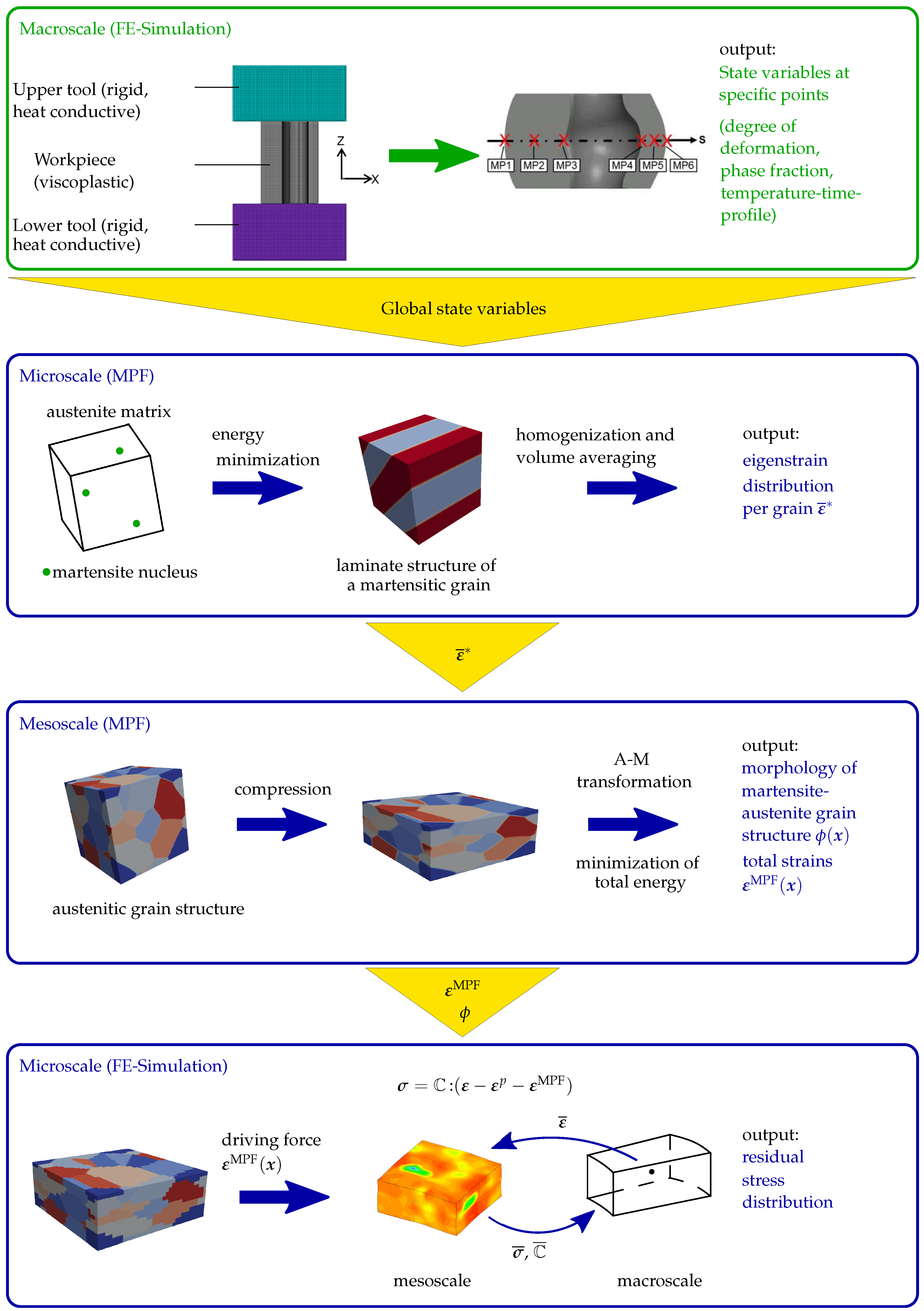
Figure 12.
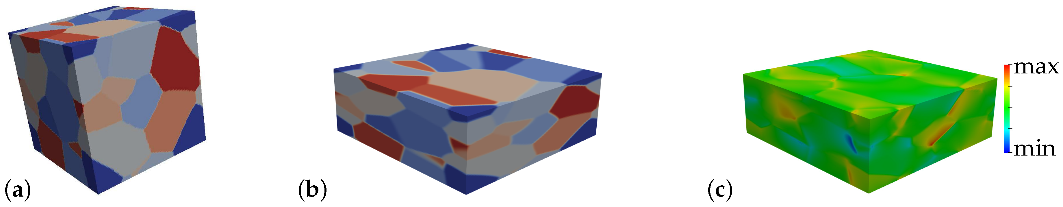
Simulation procedure of macro-, meso-, and microscale using Multi-Phase-Field Model and FE Simulation. Note that , , , denotes the total strains, the plastic strains, the mesoscopic strain distribution resulting from the A-M phase transformation and the eigenstrain distribution per grain, respectively.
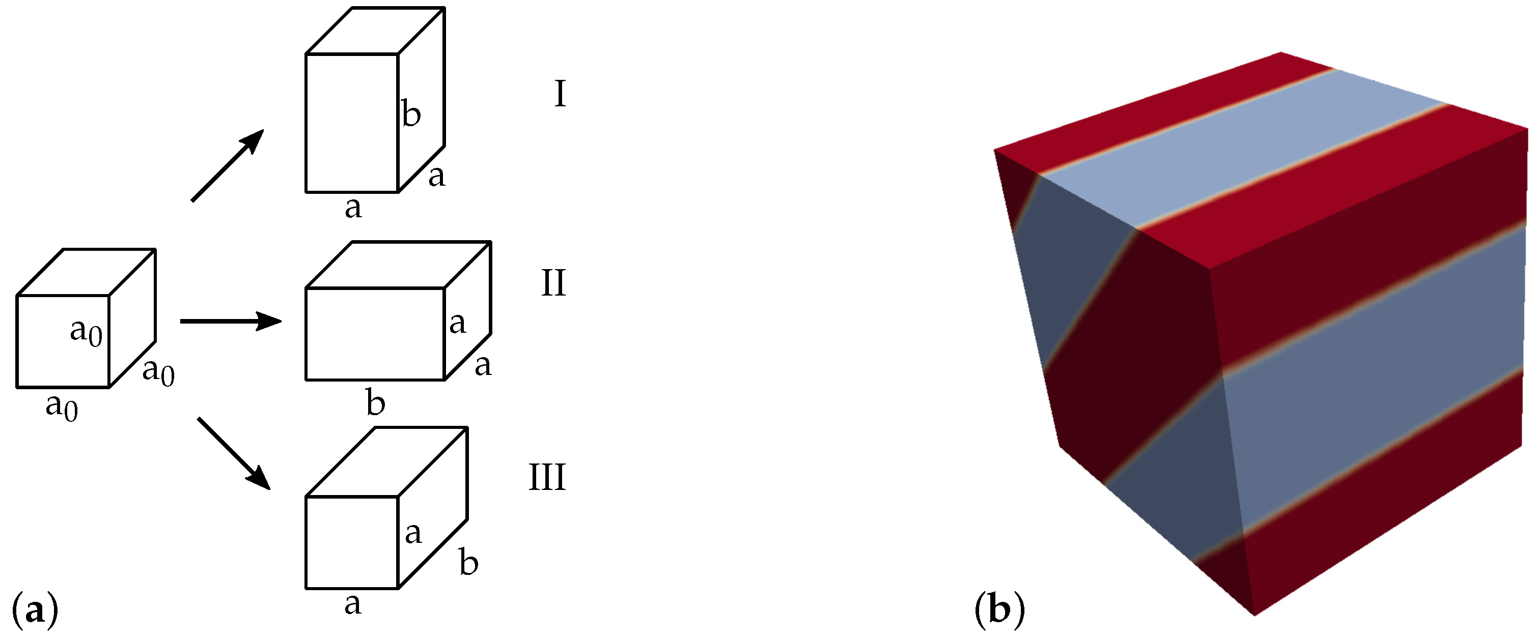
Figure 13.
(
a) Variants of martensite, cf. [
52], with
as edge length of an austenitic unit cell and
a,
b as edge length of a tetragonally transformed martensitic unit cell and (
b) laminate consisting of two variants of martensite.
Figure 14.
(a) Austenitic grain growth with different orientations for the grains, which are indicated by coloring, (b) austenitic cube with deformation regarding height and (c) first component of mesoscopic strain distribution from the MPF model .
Figure 15.
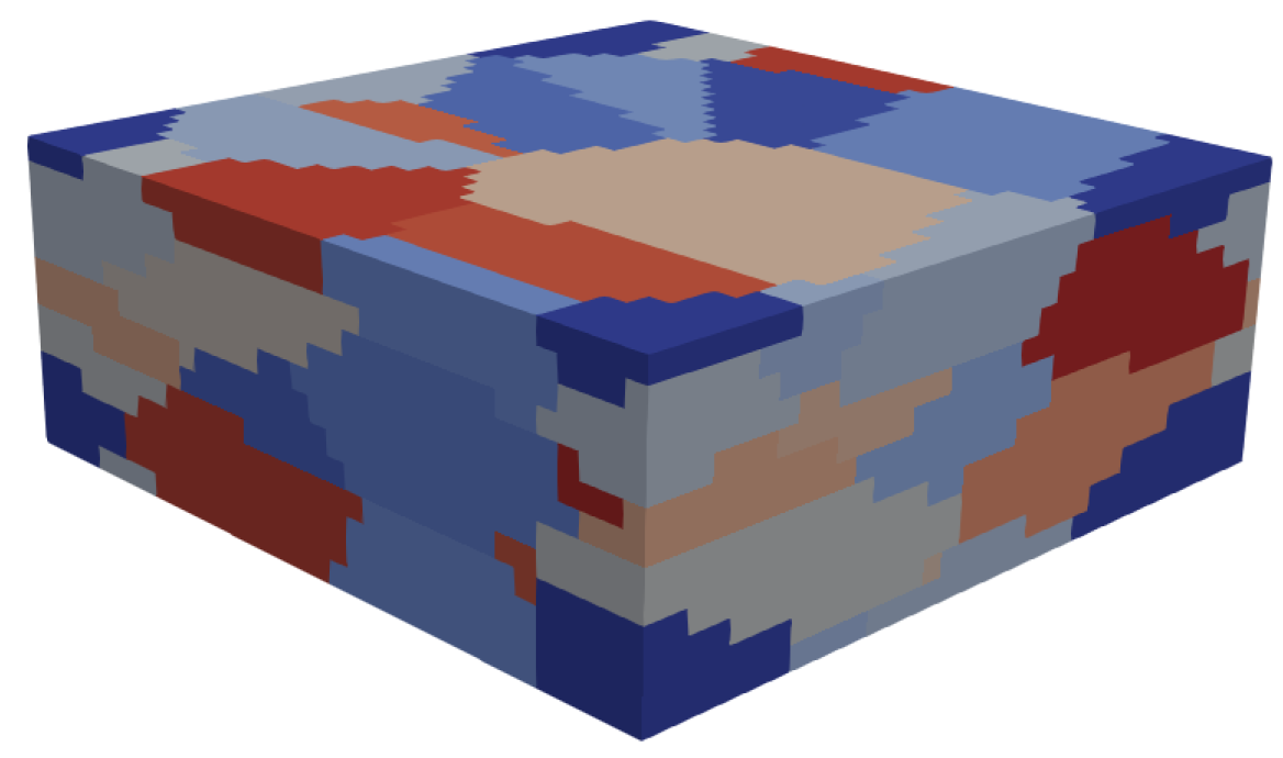
Reconstruction of the periodic mesoscopic grain structure containing 21 martensitic grains and 3 austenitic grains: FE model with 15,925 cubic elements with 136,107 nodes.
Figure 16.
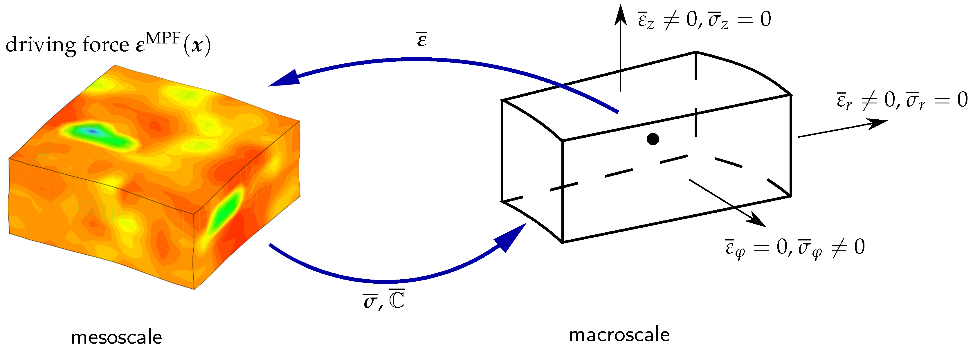
Two-scale boundary value problem for the incorporation of the strains in the FE model.
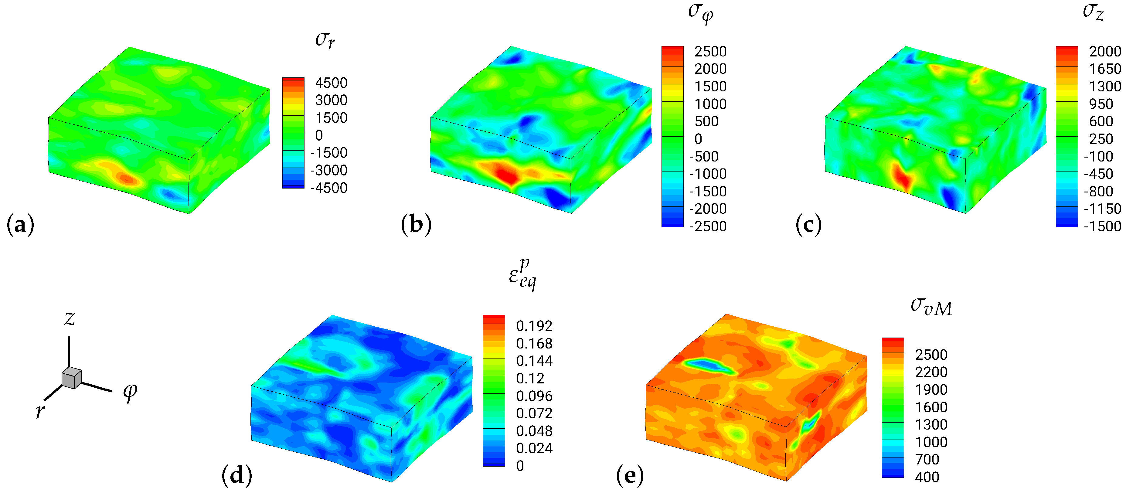
Figure 17.
(a) Radial stresses in MPa, (b) tangential stresses in MPa, (c) axial stresses in MPa, (d) equivalent plastic strains and (e) von Mises stress in MPa.
Table 1.
Chemical composition of the investigated steel alloy 1.3505 used for material data generation with JMatPro.
| Chemical Composition [wt%] | C | Si | Mn | P | S | Cr | Mo | Fe |
|---|
| 1.3505 (DIN 100Cr6) | | | | | | | | balance |
Table 2.
Parameters determined for the calculation of the flow stress
of the considered steel alloy 1.3505 according to [
49].
| A in | | | | |
|---|
| 2208 | | | | |
Table 3.
Numerically identified heat transfer coefficients between specimen and the cooling media air or water for material 1.3505.
| HTC in |
|---|
| Temperature in | Cooling Medium |
|---|
| Water (1) | Air (2) |
|---|
| 70 | | |
| 120 | | |
| 170 | 10,514.1 | |
| 220 | 10,514.1 | |
| 270 | 11,636.3 | |
| 320 | | |
| 370 | | |
| 420 | | |
| 470 | | |
| 520 | | |
| 570 | | |
| 620 | | |
| 670 | | |
| 720 | | |
| 770 | | |
| 820 | | |
| 870 | | |
| 920 | | |
| 970 | | |
Table 4.
Quantities governing the energy densities in Equations (
2) and (
3).
| i, j | components |
| , | identifier of phase-fields |
| N | total number of phase-fields |
| energy of the interface between phase-fields and |
| interface width between phase-fields and |
| chemical potential for phase-field |
| concentration of component i in phase-field |
| generalized chemical potential or diffusion potential as Lagrange multiplier for satisfying the balance of mass for each component |
| total strain of phase-field |
| eigenstrain of phase-field |
| strain of component i in phase-field |
| elasticity tensor of phase-field |
| polynomial function fulfilling and with |
| effective interfacial mobility between phase-fields and |
Table 5.
Set of equations for von Mises plasticity with exponential hardening considering additive split of strain tensor
into elastic
and plastic part
following [
58].
| kinematic | |
| stresses | |
| conjugated internal variable | |
| reduced internal dissipation | |
| yield criterion | |
| flow rule | |
| evolution of internal variables | |
| Kuhn-Tucker conditions | |
Table 6.
Material parameters for austenite and martensite for 1.3505 at temperature .
| | | | | | | h |
|---|
| | in MPa | in MPa | in MPa | in MPa | − | in MPa |
|---|
| austenite | 150,709.09 | 64,707.74 | | | | |
| martensite | 157,282.56 | 71,205.08 | 2200.0 | 2675.0 | | |
© 2019 by the authors. Licensee MDPI, Basel, Switzerland. This article is an open access article distributed under the terms and conditions of the Creative Commons Attribution (CC BY) license (http://creativecommons.org/licenses/by/4.0/).


 ,
, 


