Abstract
Mathematical descriptions of true stress/true strain curves, experimentally obtained on cylindrical specimens under hot compressive conditions, are of great importance and are widely investigated. An additional black-box modelling approach using transfer functions (TF) is tested. For tested 51CrV4 steel, a TF of third order is employed for description of true stress (output) depending on the strain rate (input). Sets of TF coefficients are determined using numerical optimization techniques for each testing temperature and strain rate. To avoid scattering of TF parameters, time in Laplacian transformation is replaced with strain, while TF input is the strain rate. Obtained models cover deformations starting practically from zero to 0.7. Average absolute relative error for models based on TF of the third order and of the second order are 0.93% and 3.64%.
1. Introduction
Mathematical models describing hot deformation behavior of metals have a long history and numerous approaches. Probable reason is needed for an even better description and prediction of metal behavior during numerous hot deformation processes serving industrial production of metallic products and semi-products in the metallic industry. Hot deformation models are generally used in CAD-CAM software’s for modelling and simulation of various hot-deformation processes (open and close die forging, hot stamping, pressing, etc.). The next very important application of these models is the prediction of roll separation force on hot rolling mills, where accuracy of roll separation force prediction is highly correlated to the strip, plate, or bar dimensional control accuracy. For accurate roll separation force models, accurate stress-strain relationships are essential [1].
Numerous modelling approaches appeared historically to describe/predict true stress: Hollomon equation [2], Johnson-Cook [3] and modified Johnson-Cook equation, Arrhenius constitutive equation, various strain compensation approaches, static strain-stress mapping with polynomials and artificial neural networks, etc. Three recent comparative studies of Mirzadeh, He and Xia [4,5,6] (each author comparing and evaluating seven, three, and three different modelling approaches, respectively) have shown, that the error (descriptive or predictive) of these models is above 6%, measured by AARE (Average Absolute Relative Error). A strain-compensation approach employed by Yang [7] on super austenitic stainless steels however result in better precision with AARE ranging from 6.65% to 0.68%. However, some older and fundamentally different modelling approaches based on differential equation(s) suggest a better match between model and prediction can be obtained with compact models with single internal state described by some kind of differential equation. Critical internal state dynamics described by the differential equation are related to static, meta-dynamic or dynamic recrystallization, and dynamic recovery. Models with internal states consider dislocation density [8,9] as internal state or additionally grain size [10] or work hardening rate [11] and exhibit promising accuracy although matching is not numerically evaluated in these research papers. A range of dedicated models is developed for prediction of onset of dynamic recrystallization (survey for these models is in Reference [10]), or determination of conditions for initiation of dynamic recrystallization [9,12,13].
Besides the torsional hot deformation test, compressive tests of cylindrical specimens at typical hot-deformation temperatures are widely used for lab-scale testing of hot workability of alloys. On experimental devices, specimens are either conductively or inductively closed-loop control heated to preset temperatures, where temperature is usually measured by thermocouple spot-welded to specimen surface. Deformation on these devices is closed-loop controlled, where position is measured typically by LVDT sensors. Typically, experiments are carried out at fixed temperature and fixed strain (deformation) rate. Force (stress) and deformation are recalculated to obtain true stress/true strain curves. Repeatability of experimentally obtained true stress-true strain curve on experimental device used in this research is around 1%. Newer experimental or supplemental approaches based on virtual fields methods offer a wider range of experimental conditions (high strain rates), and improves accuracy (specimen spatial temperature distribution). Thermal imaging on high temperature compression tests determine spatial distribution of sample temperature, e.g., see Reference [14]. Emerging experimental devices and techniques offer more and more accurate, precise and detailed insights in the hot deformation process, while established physical based models seems to have trouble to convert more precise experimental data in more precise models.
Physical based models formulations provide meaningful insight in the processes governing hot deformation. The presented TF modelling approach was designed with three aims being traced: Improve model accuracy, stress prediction for non-constant strain rate, and model applicability on the industrial level. A drawback of TF models is lost understanding of these physical underlying processes governing hot deformability, since the TF model, as used in this case, is a black-box modelling approach. Lost understanding as a consequence of the black-box approach is replaced by the TF’s model ability to capture any microstructural process influencing the stress strain response to its experimental data limitations in the range of experimental parameters limits (temperature, strain rate). Where the TF model differs, as compared to established physical based models (regarding Black-box approach), is that its parameters in frequency space s do not represent (at least not directly) physical phenomena in contrary to established physically based modelling approaches where each model parameter has its physical meaning.
This paper presents a black-box modelling approach using TF (transfer functions) for mathematical description of dynamical relation between stress and strain at typical hot working temperatures with an accuracy of about 1%. Basic expected benefit of TF is in fact that TF of nth order describes dynamic relation between input and output based on nth order differential equation. One among possible input-output configurations for description of stress-strain curve using TF has shown [15] that around 1% AARE accuracies are obtained. In this paper, it is shown that it is possible to describe stress-strain relationship starting from zero deformation to 0.7 with similar AARE slightly below 1%, but with significantly less scattered parameters. There are two main benefits of TF models use for true stress-true strain curve description beside its accuracy. The first is that the obtained model can be simply used for stress prediction of arbitrary reasonable deformation curves (inputs), and also, therefore, for industrial deformation measurements (real-time or off-line). The second benefit is that industrial-scale realizations of TFs on PLCs and PACs are widely available.
2. Materials and Methods
2.1. Steel Fabrication and Sample Preparation
Investigated specimens are made of laboratory scale produced 51CrV4 spring steel grade, hot rolled in the temperature range from 1200 °C to 1000 °C into flat bars 22 mm thick with chemical composition given in Table 1. Investigated steel grade is in this temperature range in the austenitic phase [16]. Specimens for dilatometer experiments are machined into cylinders with height and diameter of 10 mm and 5 mm, respectively. Cylinder (height) orientation are made from bar in the rolling direction. Hot compressive tests were performed on deformation dilatometer apparatus TA Instruments 805A/D (TA Instruments, New Castle, PA, USA), where specimens are inductively heated to prescribed temperatures with heating rate 10K/s, held on the temperature for an additional 10 min and then compressively deformed with preset strain rate up to the total deformation of 0.7. Experiments are carried out at five different temperatures (1000, 1050, 1100, 1150, and 1200 °C) and four strain rates (0.01, 0.1, 1, and 10 s−1). Force, displacement, specimen temperature, and heating power are measured continuously by the apparatus, while true stress-true strain curve is simultaneously calculated by machine during the experiment. A standard non-lubricated 0.1mm thick molybdenum plates are used on specimen contact surface. Obtained true stress-true strain curves are not friction corrected or filtered in any way.

Table 1.
Chemical composition of investigated 51CrV4 steel in wt. %.
2.2. Modeling Using Transfer Functions and Model Accuracy Estimation Method
Transfer functions are widely used for input-output descriptions of various electronic components, filters, other electronic assemblies, plant models description (open loop response) and closed loop response of control loops, various mechanical systems, pharmacokinetics, etc. The common point of all these systems is their dynamical relation between input and output, which can mathematically be described by differential equation(s). Observing the complex microstructural competing processes [17] in specimens of the above described experiment and the input/output response, one can assume that resulting stress response of specimen to its deformation also has a dynamical nature. Beside state-space systems and simply differential equations, transfer functions are very appropriate general tools used to mathematically describe such complex dynamical systems. The transfer function of the third order is defined as
One limitation of the use of transfer function is that it can describe response of only linear time invariable systems (LTI). In the current case, system is nonlinear in Temperature and in Strain rate. Thus, one transfer function can only describe the relation between true stress and true strain for a single pair of temperature and strain rate.
Crucial benefit of TF use for description of hot compressive stress strain curves is in fact that the processes dynamics being in time-space described by differential equation(s) is using Laplace transform in frequency space represented in simple polynomial form (Equation (1)). This means that differential equations in time-domain describing stress-strain relations using Laplace transform of then input (strain) and output (stress) signals are converted to sets of linear equations in the Laplace domain [18]. Additional benefit is a consequence of the black-box approach. Regardless, which microstructural process dominates in stress strain response, TF captures its consequences on macroscopic stress-strain curve.
In this case we use transfer function of 3rd order (1), where numerator and denominator are of the same order to assure finite response as frequency approaches infinity. In the current case, the input x(t) to transfer function is strain rate and output of transfer function is true stress (2). Instead of time, along which, normally, these simulations are performed and a true strain is used (2). One could use time instead of true strain, but the resulting transfer functions coefficients in such a case would be widely scattered depending on the range of strain rates used in the experiments. Substitution of time with strain leads to more uniform distribution of TF parameters (a3, …, a0, b3, …, b0) across a wide range of strain rates and temperatures.
For TF response calculations both MATLAB + Simulink [19] and GNU Octave [20] are used and compared. Both environments offer similar functionality for numerical calculation of Laplace transformation of input signal, calculation of response in s-space, and finally calculation of inverse Laplace transformation to obtain response back in time-space. Note that, in this case, input and output signals are actually in the strain space (Equation (2)). Coefficients of TF numerator and denominator polynomial are determined by nonlinear optimization routine “lsqnonlin” function in GNU Octave–function of “optim” toolbox. The toolbox is included by executing “pkg load ‘optim’”. MATLAB offers a function with the same name and similar syntax in the optimization toolbox.
The resulting models are valid around specific temperature and strain rate used in the experiment; temperatures (1000, 1050, 1100, 1150, and 1200) °C and strain rates (0.01, 0.1, 1, and 10 s−1). Measure of mismatch between measured and model calculated stress curves is the Average Absolute Relative Error (AARE) defined by
where is measured stress, is calculated stress, n is number of observed points of stress—strain curve and i—specific point on curve. The same measure (3) is also used by many other authors [4,5,6,7,21,22,23].
3. Results
3.1. Comparison of Measured and Model-Calculated Stress-Strain Curves
Comparison of measured and TF model-obtained true stress-true strain curves for temperatures (1000, 1050, 1100, 1150, and 1200 °C) and strain rates (0.01, 0.1, 1, and 10 s−1) is shown in Figure 1 and calculated AARE errors are given in Table 2.
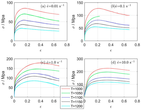
Figure 1.
Comparison of measured (dots) and 3rd order TF calculated (line) true stress-true strain for: (a) = 0.01 s−1, (b) = 0.1 s−1, (c) = 1 s−1, and (d) = 10 s−1.
Table 2.
AARE (Average Absolute Relative Error) for models based on 3rd order TF (Transfer Function).
Generally, very good agreement is obtained. What is maybe evident is some uncovered dynamics by model for some curves, e.g., Figure 1a for 1050, 1100, and 1150 °C. Analyses of temperature recording on experimental devices revealed that at least some of these deviations are caused by temperature variation of deformed sample during the deformation experiment. In the remaining cases, where temperature deviation is not the case, the proposed third order TF simply cannot cover such dynamics. Better match in such cases could be obtained by the fourth order TF, but could still not fully cover dynamics in full deformation range, since this dynamics starts at specific deformation, where oscillating behavior occurs [24]. Note that the TF calculated curves are not prediction curves, but only best obtained fit in the sense of least-squares of used transfer function to measured data. Numerical measure used to estimate the mismatch between the model calculated and measured data is AARE. Mean value of AARE for all 20 experimental conditions given in Table 2 is 0.93%. An additional note should be given for curve = 0.1 s−1 and 1050 °C (Figure 1b), where the experiment failed after deformation reached 0.23. The remaining curve is omitted, and TF parameters for this curve were only determined for deformations below 0.23.
3.2. Polynomial Transfer Function Coefficients
Transfer function of the third order is defined with, altogether, eight parameters (Equation (1)) for each experimental strain rate and temperature combination. The leading coefficient of denominator polynomial always equals 1, and thus seven coefficients are to be determined. The determined coefficients for analyzed pairs of strain rate and temperature, determined by optimizations, are listed in Table 3. Using coefficients for selected temperature and strain rate, one can determine the model in, e.g., GNU Octave(Free software, written by John W. Eaton, et. al.) or MATLAB(MATLAB 2018, The MathWorks, Natick, MA, USA) software using single command “sys = tf([a3,a2,a1,a0],[1,b2,b1,b0]);”. In GNU Octave, control package has to be loaded beforehand by executing “pkg load ‘control’”. Once TF is defined as sys object, response to strain rate equal to 1 can be calculated or plotted (in MATLAB and GNU Octave; Figure 1c) by executing command “y = step(sys,εmax)” or “step(sys,εmax)”, respectively. εmax is in both cases final strain (deformation), which in the present case is 0.7.
Table 3.
Determined coefficients of 3rd order TF polynomials (2), describing stress-strain relationship for certain temperatures T and strain rates . Coefficient b3 equals 1 and is therefore omitted.
For strain rates not equal one, commands in MATLAB and GNU Octave differ. In MATLAB, one should set ‘StepAmplitude’ option to value equal to strain rate. For example, for the model for the first row in Table 3 (T, ) = (1000, 0.01) one should execute “opt = stepDataOptions (‘StepAmplitude’, 0.01);“ before the “step(sys,εmax)” command to obtain step response for (1000, 0.01) model (Figure 1a) with coefficients given in Table 3. In Octave one should use “lsim(sys,U,t)” or “y = lsim(sys,U,t)” for plotting or calculating the step-like response of any model build from coefficients in Table 3. Note that, U and t in this case are vectors of the same size, where U is value of strain rate and t is ‘time’ vector, substituting strain “ε” with an appropriate number of calculation points, e.g., 100. One can generate such U by executing “U = 0.01.*ones(100,1);” and t by executing “t = linspace(0,0.7,100);”.
3.3. Implemantation of Transfer Functions in other Simulation and Industrial Environents
Description of dynamical systems is widely used in many simulation environments (MATLAB–Simulink, GNU Octave [20], CAD-CAM softwares, etc.) and employed in control environments for Programmable Logical Controllers (PLCs) and for Programmable Automation Controllers (PACs). MATLAB and Simulink, which are used in this paper, offers conversion of Simulink models and MATLAB functions into IEC 61131-3 compatible text code in PLC Open XML file format or others. In other words, MATLAB and Simulink functions and models and thus also TFs defined in Simulink are convertible to PLC codes.
This format is supported by IDE-s of many PLC and PAC manufacturers worldwide [25]. Thus, transfer function as used in this paper can be directly implemented on industrial automation and control devices. Besides this conversion, some PLC and PAC manufacturers offer transfer function already as a block diagram. Lastly, individual implementations of TF on various PLCs and PACs are possible within manufacturers IDEs as well.
GNU Octave, as an open-source free computational environment similar to MATLAB, also offers determination of TF via numerator and denominator coefficients in its “control” package, besides other tools for simulation, optimization, and determination in time as well as in frequency space.
TF can also be transformed to other forms of dynamical system description: Discrete transfer function (z-Transform), and continuous or discrete state-space models. Additional important aspect of stress-strain relation representation with TF is in fact that the model can be directly used as a ‘plant model’ for various controllers including forms of Model Predictive Controllers [26] or its encapsulation in other dynamical models (e.g., roll separation force models), since TF is one of the basic forms of dynamical-system response description.
3.4. Some Aspects of Strain Rate Input Signal
Experimental devices like TA Instruments 805A/D apparatus used in this case measure force (stress) and displacment (strain), but does not measure the strain rate, which is required as input for the TF model in this case. However, strain rate is usually closed-loop controlled by the apparatus to the prescribed values (e.g., 1s−1). There are at least two possibilities regarding what to use as a strain-rate signal for the TF input. One approach is to numerically calculate time derivative of measured strain signal. Expectedly, numerical derivative has quite some noise, as shown in Figure 2, but the mean values approaches the preset strain-rate, which is actually a closed loop response of controlled strain rate. Instead of noisy derivative signal, one could generate a step-like strain-rate input signal without any noise, at least for coefficients determination. In this way, simplification and faster optimization convergence is achieved. In fact, for optimization, as well as for simulation purposes generation of step-like strain rate input signal instead of numerical calculation of time-derivative of strain, turned out to be only viable way. Code for generation of step-like strain rate signal is shown in Section 3.2.
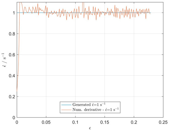
Figure 2.
Comparison of generated strain rate signal (blue) and strain rate signal obtained by numerical differentiation (red), both for = 1 s−1.
3.5. Stress Prediction for Non-Constant Strain Rates
Experimentally obtained true stress-true strain curves are obtained at constant strain rate and used for determination of TF coefficients describing the true stress-true strain relationship. Under industrial conditions, the strain rate is rarely constant and is therefore interesting to determine stress prediction to non-constant strain rate, e.g., strain measurements.
Multiplication of Equation (2) by results in . To obtain stress back in strain space, inverse Laplace transform of right side is determined by . Stress prediction for arbitrary strain rate signal is therefore calculated by (1) calculation of Laplace transform of strain rate signal (input), (2) multiplication of TF(s) and , and by (3) inverse Laplace transform of obtained product. Calculation of Laplace (1) and inverse Laplace (3) transform requires numerical determination of integral, while (2) is the algebraic computation of product of TF(s) and .
For demonstration of TF stress-strain model inherent ability to predict response (stress) to ‘arbitrary’ strain rate, three simulation experiments are made, partially inspired by different hot working machine designs used in the metallic industry or as experimental devices. This is not a model validation or calibration test, but rather a demonstration of the TF’s model abilities to predict response to some variable strain rate deformation conditions.
For all three cases strain rate starts from 10 s−1 and then (a) linearly decreases to zero, (b) decreases proportionally to square root law and (c) exponentially decreases to zero. Input strain rates (black) and TF model predicted responses (blue) for these three strain rate inputs are presented in Figure 3. Predicted stress-strain curve for linearly decreasing strain-rate (a--LIN) is similar to measured true stress-true strain profile of drop-weight experiments in Reference [27] (although they are carried out at room temperature and two decades of higher strain rates) on one hand, and similar to industrial hydraulic or screw type presses. Experiment developed for testing of sheet specimens by progressive decrease of strain rates yields more pronounced decrease of force after reaching peak force [28], which is similar to the stress-strain response on the square root law shape of the strain-rate input (b--SQRT). Exponentially decreasing strain rate profile (c--EXP) is closer to strain rate profiles obtained on crank press type hot deformation machines in industry. Calculation of such response is simply performed by execution of “y = lsim(sys,U,t);” command in MATLAB as well as in GNU Octave environment, where input vectors “U” and “t” should be properly defined to represent the desired “strain rate” form.
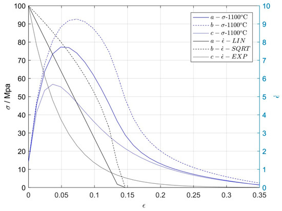
Figure 3.
Responses (σ) to linear (a), square-root (b), and exponential decline (c) off strain rate from initial 10 s−1 to zero and corresponding input strain rate curves for 1100 °C.
Two major limitations of such predictions are to be considered. (1) Deformations are non-reversible for plastic region and (2) individual model is limited for use around working conditions (strain rate and temperature). The first term is satisfied for any proper compressive deformation (rate) measurements. The second limitation can be handled by some sort of wide spread and proven “gain scheduling” technique [29] commonly used for ‘switching’ among linear models. For the case of modeling stress-strain curves using TFs, scheduling parameters are strain rate and temperature.
3.6. Zero Pole Analyses of Obtained Transfer Functions
Every transfer function of the given form (2) can be transformed into zero pole form by finding roots of numerator and denominator polynomials. Denominator roots are called poles, while numerator roots are called zeros. Dynamics of the system is dominated by poles which are closer to zero compared to others. By observing poles proximity and their position in complex plane one can estimate the required system complexity. In this case poles of system at T = 1000 °C and = 0.01 s−1 are at p1 = −225.2, p2 = −11.69, and p3 = −3.39. This means that poles p2 and p3 dominate, while p1 has little influence on dynamics. Since all three poles are negative and thus lie in left part of complex half-plane, the system response is stable [30]. Poles for different temperatures and strain rates are similarly positioned in complex plane except that some of them appear as conjugated complex pairs. Principal conclusion of zero-pole analyses is, that one could reduce TF order from third to second order by sacrificing some accuracy. To test this, we redefined TF by decreasing the order on two, performed optimizations to obtain TF polynomials, recalculated the response, and compared measured values and TF response. Comparison of TF response and measurements is shown in Figure 4 and obtained AARE errors presented in Table 4. Mean AARE of all models given in Table 4 is 3.64%. Higher mismatch between measured and second order TF calculated curves are where more dynamic components are pronounced in response (c). This is expected since second order TF can generate only two modes. Coefficients of TF polynomials for second order TF, obtained by optimization are given in Table 5.
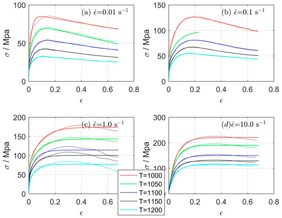
Figure 4.
Comparison of measured (dots) and 2nd order TF calculated (line) true stress-true strain for: (a) = 0.01 s−1, (b) = 0.1 s−1, (c) = 1 s−1, and (d) = 10 s−1.
Table 4.
Average absolute Relative Error (AARE) for model based on 2nd order TF.
Table 5.
Defined coefficients of 2nd order TF polynomials describing stress-strain relationship for various temperatures T and strain rates . Coefficient b2 equals 1 and is therefore omitted.
4. Discussion
Depending on the needed accuracy, one can use the second or third order transfer function for the true stress-true strain model. For more complex stress-strain curves with high AARE it might be necessary to increase TF to the fourth order (Figure 1a)-1100 °C and 1150 °C). The presented configuration of input (strain rate), output (stress) and time (strain) is not the only possible choice. Substitution of time in Laplacian transform with strain is used to reduce response dynamics, which improves optimizations convergence needed for determination of TF polynomials due to similar dynamics of models. Similar simplification is obtained by choosing the “strain rate as an input”. On the other hand, strain rate as input leads to problems regarding determination of strain rate as derivative of measured strain signal. Presented approach by artificially generated strain rate solves this problem. An alternative approach, still using the “strain rate as input” signal, but with the constant amplitude being equal to 1, leads to more scattered gain of obtained TF, as reported in Reference [15].
Some preliminary modelling approaches for using ”strain as input” to TF have shown similar accuracy as the ones presented in this paper. Major benefit of “strain as input” approach is that strain measurements, including industrial ones can be directly used as a TF input and seems more practical for industrial use. Choice of time scale or its substitution by strain leads to the same consequences, as in the case of “strain rate as input”.
True stress-true strain curve description using TF can be directly used for numeric determination of various critical conditions and points: Peak stress , numerical determination of elastic modulus [31], onset of dynamic recrystallization [12], etc.
Beside transfer functions (Laplacian transformation), which are used and discussed in this paper, one could also use other established model description forms: state space, discrete state space, discrete transfer function (Z-transformation). Many of those model forms are readily available in PLCs and PACs nowadays used on industrial level. Since many of these model forms can be transformed from one to another and/or vice-versa, similar results would probably be obtained by using remaining model forms.
The proposed TF model results in higher number of parameter for description of true stress-true strain response compared to established methods. Arrhenius equation models determine α, n, Q, and lnA and by strain compensation of these parameters with fifth order polynomial leads to altogether 4 × 6 = 24 parameters describing whole range of temperature and strain rates, see e.g., Reference [5]. Original Johnson-Cook model requires determination of only five parameters [5], improved Johnson-Cook model [5] requires determination of six parameters for whole range of strain rates and temperatures. Presented third order TF model requires seven parameters per temperature and per strain rate, while the second order TF model requires five parameters. Five temperature sets and four strain rates result in 5 × 4 × 7 = 140 parameters for the third order TF and 5 × 4 × 5 = 100 parameters for the second order TF.
Use of TF models should not be regarded as a substitute for physical based modelling approaches, but rather as a complementary method offering some additional capabilities: Simple calculation of stress for non constant strain rate inputs, improved accuracy, and fully functional support on industrial level devices.
5. Conclusions
The following conclusions can be derived from the work presented:
- Continuous type TF can accurately describe hot-deformation stress-strain relationship, but the individual model has to be used for specific temperature and strain-rate conditions.
- A disadvantage of the proposed TF model is a higher number of model parameters.
- Choices of strain or strain rate for input signal leads to comparable accuracy of obtained models. Selection of strain rate however leads to more dense roots of TF polynomials.
- Similar effect on roots of TF polynomials is obtained by substitution of time with strain in Laplacian transformation.
- Second or third order TF polynomials seem to offer appropriate dynamics for stress strain relationship description, but later offer better accuracy.
- Once TF polynomials are determined, one can easily predict strain response on any ‘reasonable’ strain-rate signal or measurement.
- Transfer Functions models are nowadays supported by most PLCs, PACs and other numerical computational environments and therefore description of stress-strain relationship by TF is supported down to the industrial level. If not by TF, one can transform TF to the preferable model form.
Author Contributions
F.V. conceptualized research and wrote article, S.M. and B.A. made dillatometer experiments, F.T. and B.A. laboratory-scale steel fabrication including hot rolling, B.P. revised and edited the paper and B.P. acquired the funding.
Funding
This research was funded by Slovenian research agency under program group P2-0050.
Conflicts of Interest
The authors declare no conflict of interest.
References
- Zhang, D.-H.; Liu, Y.-M.; Sun, J.; Zhao, D.-W. A novel analytical approach to predict rolling force in hot strip finish rolling based on cosine velocity field and equal area criterion. Int. J. Adv. Manuf. Technol. 2016, 54, 843–850. [Google Scholar] [CrossRef]
- Hollomon, J.H. Tensile deformation. Trans. AIME 1945, 12, 268–290. [Google Scholar]
- Johnson, G.R.; Cook, W.H. A Constitutive Model and Data for Metals Subjected to Large Strains, High Strain Rates, and High Temperatures; ScienceOpen, Inc.: Burlington, MA, USA, 1983; pp. 541–547. [Google Scholar]
- Mirzadeh, H. Constitutive modeling and prediction of hot deformation flow stress under dynamic recrystallization conditions. Mech. Mater. 2015, 85, 66–79. [Google Scholar] [CrossRef]
- He, A.; Xie, G.; Zhang, H.; Wang, X. A comparative study on Johnson–Cook, modified Johnson–Cook and Arrhenius-type constitutive models to predict the high temperature flow stress in 20CrMo alloy steel. Mater. Des. 2013, 52, 677–685. [Google Scholar] [CrossRef]
- Xia, Y.; Zhang, C.; Zhang, L.; Shen, W.; Xu, Q. A comparative study of constitutive models for flow stress behavior of medium carbon Cr–Ni–Mo alloyed steel at elevated temperature. J. Mater. Res. 2017, 32, 3875–3884. [Google Scholar] [CrossRef]
- Yang, L.-C.; Pan, Y.-T.; Chen, I.-G.; Lin, D.-Y.; Yang, L.-C.; Pan, Y.-T.; Chen, I.-G.; Lin, D.-Y. Constitutive Relationship Modeling and Characterization of Flow Behavior under Hot Working for Fe–Cr–Ni–W–Cu–Co Super-Austenitic Stainless Steel. Metals 2015, 5, 1717–1731. [Google Scholar] [CrossRef]
- Jorge Junior, A.M.; Balancin, O. Prediction of steel flow stresses under hot working conditions. Mater. Res. 2005, 8, 309–315. [Google Scholar] [CrossRef]
- Kugler, G.; Turk, R. Modeling the dynamic recrystallization under multi-stage hot deformation. Acta Mater. 2004, 52, 4659–4668. [Google Scholar] [CrossRef]
- Orend, J.; Hagemann, F.; Klose, F.B.; Maas, B.; Palkowski, H. A new unified approach for modeling recrystallization during hot rolling of steel. Mater. Sci. Eng. A 2015, 647, 191–200. [Google Scholar] [CrossRef]
- Lin, Y.C.; Liu, G. A new mathematical model for predicting flow stress of typical high-strength alloy steel at elevated high temperature. Comput. Mater. Sci. 2010, 48, 54–58. [Google Scholar] [CrossRef]
- Poliak, E.I.; Jonas, J.J. A one-parameter approach to determining the critical conditions for the initiation of dynamic recrystallization. Acta Mater. 1996, 44, 127–136. [Google Scholar] [CrossRef]
- Zhang, C.; Zhang, L.; Shen, W.; Liu, C.; Xia, Y.; Li, R. Study on constitutive modeling and processing maps for hot deformation of medium carbon Cr–Ni–Mo alloyed steel. Mater. Des. 2016, 90, 804–814. [Google Scholar] [CrossRef]
- Zheng, L.; Lee, T.L.; Liu, N.; Li, Z.; Zhang, G.; Mi, J.; Grant, P.S. Numerical and physical simulation of rapid microstructural evolution of gas atomised Ni superalloy powders. Mater. Des. 2017, 117, 157–167. [Google Scholar] [CrossRef]
- Vode, F.; Burja, J.; Tehovnik, F.; Arh, B. Lumped paramter model with inner state variables for modelling hot deformability of steels. Metalurgija 2017, 56, 111–114. [Google Scholar]
- Zhang, L.; Gong, D.; Li, Y.; Wang, X.; Ren, X.; Wang, E.; Zhang, L.; Gong, D.; Li, Y.; Wang, X.; et al. Effect of Quenching Conditions on the Microstructure and Mechanical Properties of 51CrV4 Spring Steel. Metals 2018, 8, 1056. [Google Scholar] [CrossRef]
- Wang, Z.; Xie, F.; Lai, C.; Li, H.; Zhang, Q.; Luo, D. High Temperature Hot Deformation Behavior and Constitutive Model Construction of High Quality 51CrV4 Spring Steel. In Chinese Materials Conference; Springer: Singapore, 2018; pp. 191–199. [Google Scholar]
- Gavin, H.P. Linear Time-Invariant Dynamical Systems; Duke University: Durham, NC, USA, 2018. [Google Scholar]
- MATLAB, + Simulink2018a; The MathWorks, Inc.: Natick, MA, USA, 2018.
- Eaton, J.W.; Bateman, D.; Hauberg, S. GNU Octave, version 4.2.2; Network Theory: London, UK, 2017. [Google Scholar]
- Akbari, Z.; Mirzadeh, H.; Cabrera, J.-M. A simple constitutive model for predicting flow stress of medium carbon microalloyed steel during hot deformation. Mater. Des. 2015, 77, 126–131. [Google Scholar] [CrossRef]
- Wu, H.-Y.; Yang, J.-C.; Zhu, F.-J.; Wu, C.-T. Hot compressive flow stress modeling of homogenized AZ61 Mg alloy using strain-dependent constitutive equations. Mater. Sci. Eng. A 2013, 574, 17–24. [Google Scholar] [CrossRef]
- Mirzadeh, H. Physically based constitutive description of OFHC copper at hot working conditions. Met. Mater. 2016, 53, 105–111. [Google Scholar] [CrossRef]
- Won Lee, H.; Im, Y.-T. Numerical modeling of dynamic recrystallization during nonisothermal hot compression by cellular automata and finite element analysis. Int. J. Mech. Sci. 2010, 52, 1277–1289. [Google Scholar] [CrossRef]
- Mazur, P.; Chmiel, M.; Czerwinski, R. Central processing unit of IEC 61131-3-based PLC. IFAC-PapersOnLine 2016, 49, 454–459. [Google Scholar] [CrossRef]
- Clarket, D.W.; Mohtadit, C.; Tuffs, P.S. Generalized Predictive Control Algorithm* Part, I. The Basic; Elsevier: New York, NY, USA, 1987; Volume 23. [Google Scholar]
- Abed, F.; Abdul-Latif, A.; Yehia, A.; Abed, F.; Abdul-Latif, A.; Yehia, A. Experimental Study on the Mechanical Behavior of EN08 Steel at Different Temperatures and Strain Rates. Metals 2018, 8, 736. [Google Scholar] [CrossRef]
- Enginsoy, H.; Bayraktar, E.; Kurşun, A.; Enginsoy, H.M.; Bayraktar, E.; Kurşun, A. A Comprehensive Study on the Deformation Behavior of Hadfield Steel Sheets Subjected to the Drop Weight Test: Experimental Study and Finite Element Modeling. Metals 2018, 8, 734. [Google Scholar] [CrossRef]
- Leith, D.J.; Leithead, W.E. Survey of gain-scheduling analysis and design. Int. J. Control 2000, 73, 1001–1025. [Google Scholar] [CrossRef]
- Michael, S.; Triantafyllou, F.S.H. Maneuring and Control of Marine Vehicles; Massachusetts Institute of Technology: Cambridge, MA, USA, 2003. [Google Scholar]
- Suttner, S.; Merklein, M. A new approach for the determination of the linear elastic modulus from uniaxial tensile tests of sheet metals. J. Mater. Process. Technol. 2017, 241, 64–72. [Google Scholar] [CrossRef]
© 2019 by the authors. Licensee MDPI, Basel, Switzerland. This article is an open access article distributed under the terms and conditions of the Creative Commons Attribution (CC BY) license (http://creativecommons.org/licenses/by/4.0/).