Direct Macroscopic Modeling of Grain Structure and Macrosegregation with a Cellular Automaton–Finite Element Model


Key Laboratory for Advanced Materials Processing Technology, Ministry of Education, School of Materials Science and Engineering, Tsinghua University, Beijing 100084, China
*
Author to whom correspondence should be addressed.
Metals 2019, 9(2), 177; https://doi.org/10.3390/met9020177
Submission received: 18 January 2019
/
Revised: 29 January 2019
/
Accepted: 31 January 2019
/
Published: 2 February 2019
Abstract
:Grain structure and macrosegregation are two main factors determining mechanical properties of components and are strongly coupled during alloy solidification. A two-dimensional (2D) cellular automaton (CA)–finite element (FE) model is developed to achieve a direct macroscopic modeling of grain structure and macrosegregation during the solidification of binary alloys. With the conservation equations of mass, momentum, energy, and solute solved by a macroscopic FE model and the grain structure described by a microscopic CA model, a two-way coupling between the CA and FE models is applied. Furthermore, the effect of the fluid flow on the dendrite tip growth velocity is considered by modified dendrite tip growth kinetics. The CAFE model is applied to a quasi-2D benchmark solidification experiment of a Sn–3.0wt.%Pb alloy, and the grain structure and macrosegregation are predicted simultaneously. It is demonstrated that the model has a capacity to describe the undercooling ahead of the growth front. The growth directions of columnar grains, grain sizes, and columnar-to-equiaxed transition (CET) position are obviously modified by the fluid flow, and obvious segregated channels almost aligned with the orientations of the columnar grains are found. Qualitatively good agreement is obtained between the predicted segregation profiles and experimental measurements.
1. Introduction
Solidification is a process to fabricate raw materials or even products, playing an important role in the manufacturing industry. Macrosegregation (i.e., composition heterogeneities of alloying elements over a larger scale than the microstructure) and grain structure are two main factors determining mechanical properties of components, and they are strongly coupled during the solidification of alloys. On one hand, the distributions of the temperature and solute concentrations have a significant influence on the development of the grain structure. On the other hand, the undercooling and interface morphology during the development of the grain structure remarkably affect the fluid flow, thus the heat and mass transfer. In order to achieve a deep understanding of the interaction between the grain structure and macrosegregation and to give an accurate prediction, numerical models are required to give a coupling between the solution of conservation equations of mass, momentum, energy, and solute, and the development of the grain structure.
Several modeling approaches were developed in the past decades: direct microscopic modeling, indirect microscopic modeling, indirect macroscopic modeling, and direct macroscopic modeling. Direct microscopic modeling tracks the development of phase interfaces by methods of front tracking [1], phase field [2,3], cellular automaton [4,5], volume averaging with interface tracking [6,7], or level set [8]. Although precise distributions of phases and compositions can be obtained, it is difficult for them to be applied to industrial-scale castings due to the extremely high computation cost. Indirect microscopic modeling depicts the average phase fractions and compositions by volume averaging over each independent phase. It can be embedded in direct macroscopic modeling to simplify the inner microstructure of each grain. Indirect macroscopic modeling is currently the most popular approach to industrial-scale castings [9,10,11,12,13,14]. It solves one or several sets of conservation equations averaged over a representative elementary volume for the heat and mass transfer with thermodynamic considerations of the solidification [15], but the microstructure is not directly simulated. As a consequence, direct macroscopic modeling has been proposed to make a compromise between such a coupling and the computation cost. It solves the conservation equations at the macroscopic scale, and tracks the limit of the mushy zone and the liquid at the mesoscopic scale, rather than the phase interfaces. Thus, the macrostructure and macrosegregation can be predicted simultaneously. Although the complicated morphology of phase interfaces is not described, the crystallographic orientation and the effect of the fluid flow can be well incorporated into the grain growth, making it sufficiently advanced and applicable to industrial applications [16,17,18].
Recently, a new quasi-2D benchmark experiment model was designed to accurately control the cooling rate and horizontal temperature gradient using a closed-loop controlled temperature measurement system [19]. Various solidification experiments [20,21,22] were performed based on the tin–lead (Sn–Pb) alloys due to their strong segregation tendency and operability in the laboratory, giving better experimental benchmarks for numerical validation. This contribution is devoted to achieving a direct macroscopic modeling with a 2D cellular automaton–finite element (CAFE) model, which is an extension of a newly developed FE model by the authors [23] for the prediction of macrosegregation during the solidification of binary alloys. The CAFE model is applied to the solidification benchmark experiment of a Sn–3wt.%Pb alloy [22], in which a fully developed fluid flow is initiated and a columnar-to-equiaxed transition (CET) occurs. The grain structure and macrosegregation are predicted simultaneously. The interaction between the fluid flow and the grain structure, as well as the effect of the orientations of columnar grains on the macrosegregation, are investigated in detail.
2. Model Descriptions
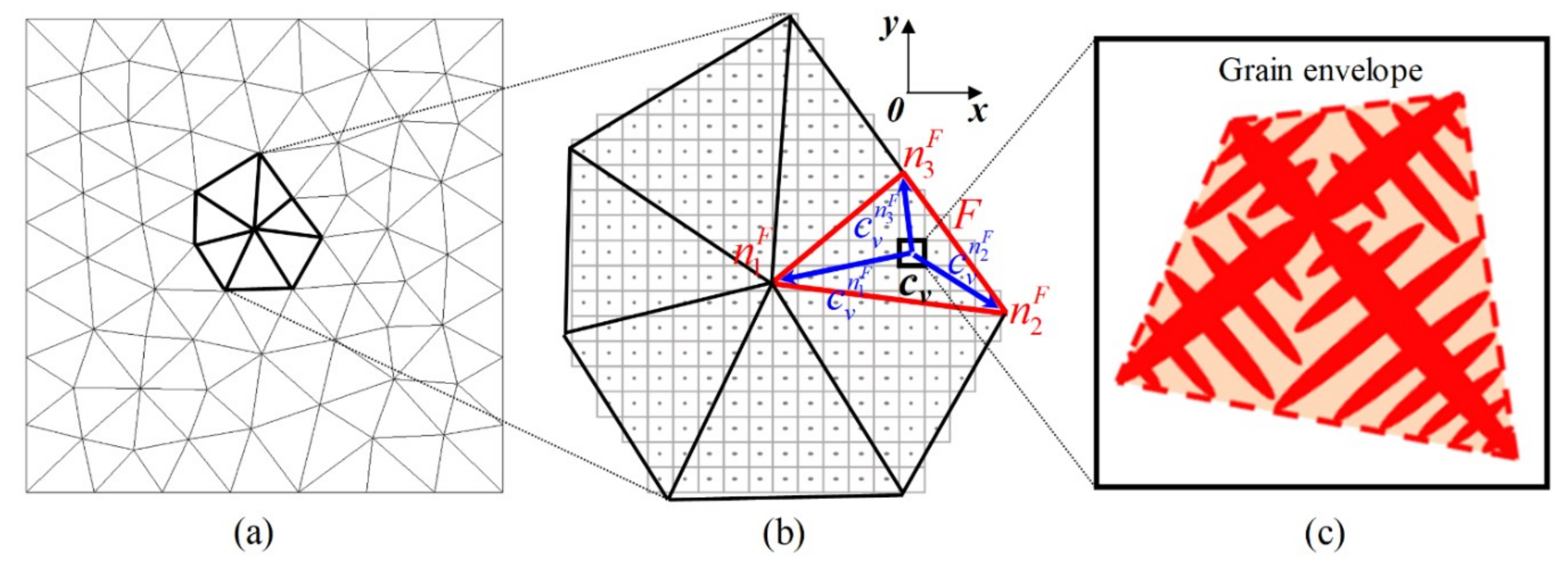
The CAFE model is based on a macroscopic FE model and a microscopic CA model, and a coupling between them is implemented. Figure 1 schematizes different length scales and their relationship included in this model. The macroscopic scale is represented by an FE grid of triangular elements, where macroscopic conservation equations of mass, momentum, energy, and solute are solved (Figure 1a). The microscopic scale is expressed by a CA grid of square cells (Figure 1b), in which the development of the grain structure is described. Neglecting the dendrite morphology, each grain is simplified by an envelope outlining the dendrite tip positions (Figure 1c). For cubic crystalline materials, the grain envelope is characterized by a quadrilateral shape in 2D case and an octahedral shape in 3D case. Only the nucleation and growth of the primary solid phase is considered, and the grain boundary wetting [24,25] is ignored.
As shown in Figure 1b, the CA and FE grids are completely superimposed. In present formulation, linear triangular element is used. Each cell v, located in a given triangular element F defined by nodes , is uniquely defined by its center coordinates, . In order to exchange information between cell v and the FE nodes , linear interpolation coefficients, , are defined. Thus, a variable available at the nodes of element F, , can be interpolated to obtain the corresponding value at cell v, , by:
Similarly, a variable calculated at the CA grid can be projected onto the FE grid. For example, the value of a variable at an FE node n, , can be obtained by the following summation over the values at all the cells, , seen by the FE node n, :
For the node shown in Figure 1b, is the number of all the cells drawn.
2.1. Macroscopic FE Model
In present formulation, a “minimal” model [26] is considered for the solidification of binary alloys. It requires the solution of coupled conservation equations averaged over a representative elementary volume considering a mixture of the solid and liquid phases. With no other phase being present, the volume fractions of the liquid, , and the solid, , always satisfy the correlation . Furthermore, the solid phase is fixed and nondeformable. Thus, the system of macroscopic equations is defined by the conservations of the total mass, momentum of the liquid phase, energy, and solute as follows:
Total mass concentration:
where is the volume-averaged velocity. In this case, it reduces to , with being the volume-averaged intrinsic velocity of the liquid phase.
Momentum conservation for the liquid phase:
where is the intrinsic liquid pressure, the time, the dynamic viscosity of the liquid, and the gravity. Assuming constant densities, and , for the liquid and solid phases, respectively, the density, , is given by . The density in the buoyancy term, , is defined by the Boussinesq approximation:
where and are thermal and solutal expansion coefficients, respectively. and are reference temperature and reference composition, respectively. The isotropic permeability in the mushy zone, , is assumed and defined by the Carman–Kozeny relation:
where is the secondary dendrite arm spacing.
Energy conservation:
where is the volume-averaged specific enthalpy per unit mass, and the volume-averaged temperature. The average thermal conductivity, , and the average specific heat, , are given by and , respectively. Thus, the relation between the volume-averaged specific enthalpy and temperature can be expressed as:
where is the latent heat of fusion per unit mass.
Solute conservation:
where is the volume-averaged mass concentration, the volume-averaged mass concentration in the liquid phase, and the diffusion coefficient of the solute element in the liquid phase.
In addition, a microsegregation model is used to close the above conservation equations. Here, the lever rule is applied and given as follows:
where is the volume-averaged mass concentration in the solid phase, the partition coefficient, the melting temperature of pure solvent, and the liquidus slope.
2.2. Microscopic CA Model
2.2.1. Nucleation
A state index, is defined for each CA cell v to identify the phase and neighborhood of cell v. By modifying the index, the development of the grain structure during solidification can be tracked. The state index is defined as follows:
- , when cell v is liquid;
- , when cell v is not liquid, but at least one of its nearest neighboring cells, , is still liquid;
- , when cell v is not liquid, and all its nearest neighboring cells, , are not liquid; where is the number of the first and second nearest neighboring cells of cell v, thus .
In present formulation, only the nucleation and growth of the primary solid phase are accounted for. Nucleation sites defined by a Gaussian distribution [27] are considered for the bulk melt and the surfaces in contact with the melt, for which the three adjustable nucleation parameters are denoted by (, , ) and (, , ), respectively. As a result of 2D approximation, the maximum volume density (m−3) and maximum surface density (m−2) are converted into the maximum surface density (m−2) and maximum linear density (m−1), respectively, by stereological relationships [28]. For a cell v containing a nucleation site, a critical nucleation undercooling, , and a random crystallographic orientation, , are attributed according to the corresponding Gaussian distribution. During solidification, if a cell v containing a nucleation site is still liquid () and its undercooling is greater than the critical nucleation undercooling , a nucleation event will take place. Then, the state indexes of all CA cells are updated according to the definition given above.
2.2.2. Growth
Once a CA cell is nucleated or engulfed by a growing grain envelope, it becomes mushy and a mushy zone starts to develop within the cell. In present 2D case, the decentered quadrilateral growth algorithm proposed by Guillemot and Gandin [16,17] is adopted. The evolution of a grain envelope is reduced to the capture of the neighboring cells. For a growing cell v, a quadrilateral growth shape is defined by the lengths of four half-diagonals corresponding to the four preferential orientations and the angle between the preferential orientation and the ox axis. Assuming that the areas of the current growth shape, the minimal growth shape, and the maximal growth shape are , , and , respectively, the volume fraction of the mushy zone within cell v is calculated by:
Then, the volume fraction of solid within cell v can be expressed by:
where is the internal volume fraction of solid within the current growth shape.
2.2.3. Dendrite Tip Growth Kinetics
The dendrite tip growth kinetics proposed by Gandin et al. [29], which is an extension of the well-known Lipton-Glicksman-Kurz (LGK) model [30], is adapted to calculate the growth velocities of the four half-diagonals of a growth shape in the presence of fluid flow independently. For a growing cell v, the total undercooling is calculated firstly by:
where is the liquid composition far from the solid/liquid interface, and the temperature. Assuming that the kinetics undercooling is negligible, the total undercooling can be split into three contributions, namely:
where , and represent the thermal undercooling, solutal undercooling, and curvature undercooling, respectively, which are expressed as follows [30]:
where is the dimensionless thermal supersaturation, the dimensionless solutal supersaturation, the dendrite tip radius, the Gibbs–Thomson coefficient, and the liquid composition at the solid/liquid interface. For the thermal supersaturation , Ivantsov correlation [30] is used:
where is the thermal Peclet number, the exponential integral function, the dendrite tip velocity, and the thermal diffusivity. For the solutal supersaturation , the boundary layer correlation proposed by Gandin et al. [29] is applied:
with A = 0.5773, B = 0.6596, C = 0.5249, where is the solutal Peclet number, the dimensionless Reynolds number, the Schmidt number, the magnitude of the fluid flow velocity far from the interface , the angle between the fluid flow direction and the four preferential orientations, and the kinematic viscosity. It is notable that a purely diffusive regime is retrieved when the magnitude of the fluid flow velocity or the angle is reduced to zero, which is the case of the LGK model [30].
The marginal stability criterion is used to approximate the dendrite tip radius by the minimum stable wavelength [30], resulting in the following relationship between the dendrite tip radius and the dendrite tip velocity :
where is the marginal stability constant taken as .
The temperature , the liquid composition far from the interface and the fluid flow velocity far from the interface are interpolated at cell v from the corresponding entities at the nodes of element F containing cell v. Based on the above equations, an iterative method is used to calculate the dendrite tip growth velocity.
2.3. Coupling Strategy
Due to the different stability requirements, a large time step, , is used for the macrocalculations, and another small time step, , for the microcalculations. Two time-stepping loops with different time steps are used for the FE and CA calculations. The micro time step is adjusted automatically to make sure that the growth of the dendrite tip within one micro time step does not exceed one CA cell size, , resulting in the following limitation:
where is the maximum of the dendrite tip growth velocities in the four preferential orientations over all the growing cells ( and ), and is a parameter introduced to ensure a correct prediction for the growth competition of columnar grains [31].
The macroscopic equations are solved according to the literature [23]. Once the variations of the master variables, such as the average enthalpy, , composition, , and liquid velocity, , over one macro time step at the FE nodes are available, the corresponding variations of the average enthalpy, , composition, , and liquid velocity, , over one micro time step are firstly interpolated in time by:
where and are the variations over the macro and micro time steps, respectively. Then, a two-way coupling between the FE and CA models is applied. On one hand, the variations of the master variables, such as the average enthalpy , composition , and liquid velocity at the CA cells are interpolated from the corresponding entities (i.e., , and ) at the FE nodes using Equation (1) at the start of each micro time step. The conversion of the new enthalpy, , and composition, , to the average temperature, , and the internal volume fraction of solid, , are performed at the CA cells with Equation (8) and the lever rule Equations (10)–(12). On the other hand, the volume fraction of liquid, , and average temperature, , at the FE nodes are fed back from the CA calculations at the end of each micro time step. With the new calculated volume fraction of liquid , the liquid composition at the FE nodes is updated using Equation (11).
3. Results and Discussion
A quasi-2D benchmark solidification experiment of a Sn–3wt.%Pb ingot under natural convection [22] is considered in this section. As shown in Figure 2, an ingot with 100 mm in length (along the x axis), 60 mm in height (along the y axis), and 10 mm in thickness (not shown in present 2D case) was melted and solidified under the controlled thermal conditions by left-hand-side (LHS) and right-hand-side (RHS) heat exchangers, with the opposite greatest surfaces of the ingot, with dimensions of 60 mm × 10 mm, placed vertically. Assuming that a quiescent melt with homogeneous temperature and composition is first obtained at 260 °C, the experimental procedure is simplified for a better description as follows: (1) setting the temperatures of the LHS and RHS heat exchangers with 270 °C and 250 °C, respectively, to apply a temperature difference of 20 °C, suggested by Boussaa et al. [22]; (2) holding the temperatures of the two heat exchangers for 1000 seconds to obtain stabilized temperature and fluid flow fields in the melt; (3) cooling both the LHS and RHS heat exchangers with a cooling rate CR = 0.03 °C/s, until the ingot is completely solidified. The cooling rate is selected as slow enough to form a significant segregation. The parameters used in present simulations are given in Table 1.
3.1. Dendrite Tip Growth Velocity in the Presence of Fluid Flow
Since the temperature, composition, and liquid velocity change with time and space during the solidification of alloys, the dendrite tip growth kinetics are required to give a dendrite tip growth velocity based on the local temperature, composition, and liquid velocity of each growing CA cell. In order to ensure the reliability of the present CAFE model, the modified dendrite tip growth kinetics defined by Equations (15)–(24) are first validated with respect to Sn–Pb alloys with fluid flow. Figure 3 and Figure 4 show the comparisons of the dendrite tip growth velocity of Sn–Pb alloys calculated by present correlation and the correlation given by Ananth and Gill [32], which yield exact solutions based on several flow approximations. A good agreement is obtained. In addition, the effect of the angle between the dendrite growth direction and the liquid velocity vector on the dendrite tip growth velocity is shown in Figure 5. It is notable that the maximal and minimal growth velocities are obtained in the upstream direction () and downstream direction () in the presence of fluid flow, respectively. In the absence of fluid flow, the growth velocity is equivalent in all directions.
3.2. Evolution of the Temperature and Solid Fraction Fields
The temperature and solid fraction fields obtained by the present CAFE model are illustrated in this section. Figure 6 shows the temperature distributions at selected instants. At 1000 s (Figure 6a), that is, the end time of stage (2) for the stabilization of the temperature and fluid flow fields, the isotherms present a stratified core at the center and vertical layers near the LHS and RHS walls. In the stratified core, the temperature increases with the increasing height, indicating a clockwise circulation of the fluid flow because of high temperature on the LHS wall. With both the LHS and RHS heat exchangers cooling down since 1000 s, the stratification characteristic of the isotherms is maintained until 1750 s (Figure 6b), when a solidification front starts to develop from the RHS wall to the left. With the solidification front developing, the isotherms in the right half and those in the left half become denser and sparser, respectively, which indicates a large temperature gradient in the mushy zone and a small one in the liquid zone, respectively, as shown in Figure 6c,d. Due to the instability of the growth front, the isotherms near the RHS wall are less smooth. At 2500 s (Figure 6e), the number of the isotherms in the left half of the ingot is very few, and the highest temperature appears at the position about a third of the length to the LHS wall, indicating that another solidification front will develop from the LHS wall to the right. Upon further cooling, the isotherms in the left part of the ingot become denser gradually and merge with the isotherms in the right part of the ingot finally at the position about a third of the length to the LHS wall, as shown in Figure 6f.
The solid fraction fields predicted at selected instants after the solidification are given in Figure 7. It is clearly shown that the first solidification front is initiated on the RHS wall and develops toward the left (Figure 7a,b), and the second solidification front starts to progress from the LHS wall to the right (Figure 7c,d). The two solidification fronts impinge at the position about a third of the length to the LHS wall, where the liquid is the last to solidify. The solid fraction profiles are also unsmooth. In order to compare the positions of the solidification fronts with those obtained in equilibrium solidification without the undercooling, a purely macroscopic FE simulation is also performed with the CA model disabled. The profiles corresponding to the solid fraction of 0.0001 obtained by the present CAFE model and the FE simulation are drawn in white and red to trace the solidification fronts, respectively. As shown in Figure 7a–c, the solidification fronts given by the present CAFE model (white profiles) overall fall behind those predicted by the FE simulation (red profiles) due to the presence of the undercooling. In Figure 7d, however, the solidification fronts given by the present CAFE model (white profiles) advance faster than those obtained by the FE simulation (red profiles), which may be attributed to a quite different distribution of Pb concentration.
In order to give a closer insight into the solidification process, the cooling curves and the solid fraction evolutions obtained by the present CAFE model at the four locations P1–P4 (shown in Figure 2) are compared with those given by the FE simulation, as shown in Figure 8. In both simulations, the solidification starts in the sequence of P4, P3, P1, and P2, and finishes in the sequence of P4, P3, P2, and P1. For the cooling curves, little difference is shown between the two simulations. The cooling curve at each location shows a great oscillation when it is in liquid state, which indicates a significant oscillation in the fluid flow. For the solid fraction evolutions, however, the results predicted by the present CAFE model at all the four locations P1–P4 obviously fall behind those given by the FE simulation, and a little more liquid undergoes the eutectic transformation finally.
3.3. Interaction between the Fluid Flow and Grain Structure
In order to clarify the effect of the fluid flow on the dendrite tip growth kinetics, the grain structure and fluid flow obtained by the present CAFE model are compared with those given by a degenerated CAFE simulation, in which the effect of the fluid flow on the dendrite tip growth kinetics is disabled. The results are presented in Figure 9 with a strong interaction between the grain structure and fluid flow. At 2000 s (Figure 9a1,a2), the fluid flow is characterized by a main clockwise convection circulation at the center of the liquid zone and several small convection circulations at the corners of the liquid zone and inside the main convection circulation. The maximal velocity is about 0.024 m/s. Columnar grains in an array have been nucleated on the RHS wall and develop toward the left. With the columnar grains advancing, the main convection circulation also moves toward the left, as shown in Figure 9b1,b2 at 2300 s. With further cooling, new equiaxed grains nucleate ahead of the columnar grains or on the LHS wall due to the decreasing temperature gradient in the liquid zone and the increasing volume of undercooled liquid, as shown in Figure 9c1,c2 at 2500 s. At the same time, the maximal velocity decreases from about 0.012 m/s to about 0.003 m/s due to the increasing permeation resistance in the mushy zone. These equiaxed grains develop quickly and impinge the growing columnar grains finally, resulting in a CET, as shown in Figure 9d1,d2 at 3900 s.
Although little difference is shown in the flow fields obtained by the present CAFE model and the degenerated CAFE simulation disabling the effect of the fluid flow on the dendrite tip growth kinetics, two significant differences can be found in the grain structures. Firstly, an obvious upward inclined columnar structure from the RHS wall to the left is predicted by the present CAFE model (Figure 9a1–d1). This is attributed to the downward inclined liquid flow ahead of the growth front. As the growth velocity in the upstream direction is greater than that in the downstream direction, the grains with one of the four preferential orientations opposite to the flow direction can adopt a smaller undercooling and survive in the competition with other grains. Thus, the columnar grains extend faster in the direction opposite to the fluid flow, resulting in the current grain selection. In the degenerated CAFE simulation (Figure 9a2–d2), however, the columnar grains are only slightly upward inclined in the lower right part of the ingot, which is caused by the slightly upward inclined temperature gradient (as shown in Figure 6). Secondly, the final equiaxed grains are obviously finer and the CET position is farther away from the LHS wall in the degenerated CAFE simulation. This is because a purely diffusive regime is retrieved in the calculation of dendrite tip growth kinetics, resulting in a smaller dendrite tip growth velocity than that in the present CAFE model. Thus, a larger volume of undercooled liquid forms and an earlier nucleation of new equiaxed grains occurs.
3.4. Macrosegregation
The segregations maps obtained by the present CAFE model, the degenerated CAFE simulation disabling the effect of the fluid flow on the dendrite tip growth kinetics, and the FE simulation disabling the CA model at selected instants are compared in Figure 10. It is demonstrated that the segregation maps are generally consistent. Once the first solidification front is initiated on the RHS wall, a negative segregation pocket and a positive segregation band develop from the RHS wall to the left at the top and bottom part of the ingot, respectively, as shown in Figure 10a1–b1,a2–b2,a3–b3. Since the initialization of the second solidification front on the LHS wall, another negative segregation pocket and another positive band develop toward the right at the top and bottom part of the ingot, respectively, as shown in Figure 10c1–d1,c2–d2,c3–d3. The two negative segregation pockets and the two positive segregation bands both impinge at the position about a third of the length to the LHS wall, forming a vertical Pb-rich plume, as shown in Figure 10d1,d2,d3. Quantitatively, significant differences can be concluded in two aspects. Firstly, comparing the segregation maps obtained by the present CAFE model (Figure 10a1–d1) with those given by the FE simulation (Figure 10a3–d3), the segregation maps obtained by the present CAFE model show a lower positive segregation band along the bottom wall, and the segregated channels beside the plume and the negative segregation chunk predicted by the FE simulation at the lower right corner are not found. Secondly, comparing the segregation maps obtained by the present CAFE model (Figure 10a1–d1) with those given by the degenerated CAFE simulation (Figure 10a2–d2), more obvious segregated channels almost aligned with the orientations of the columnar grains are predicted by the present CAFE model in the right of the plume, which is attributed to the introduction of the fluid flow in the calculation of dendrite tip growth kinetics.
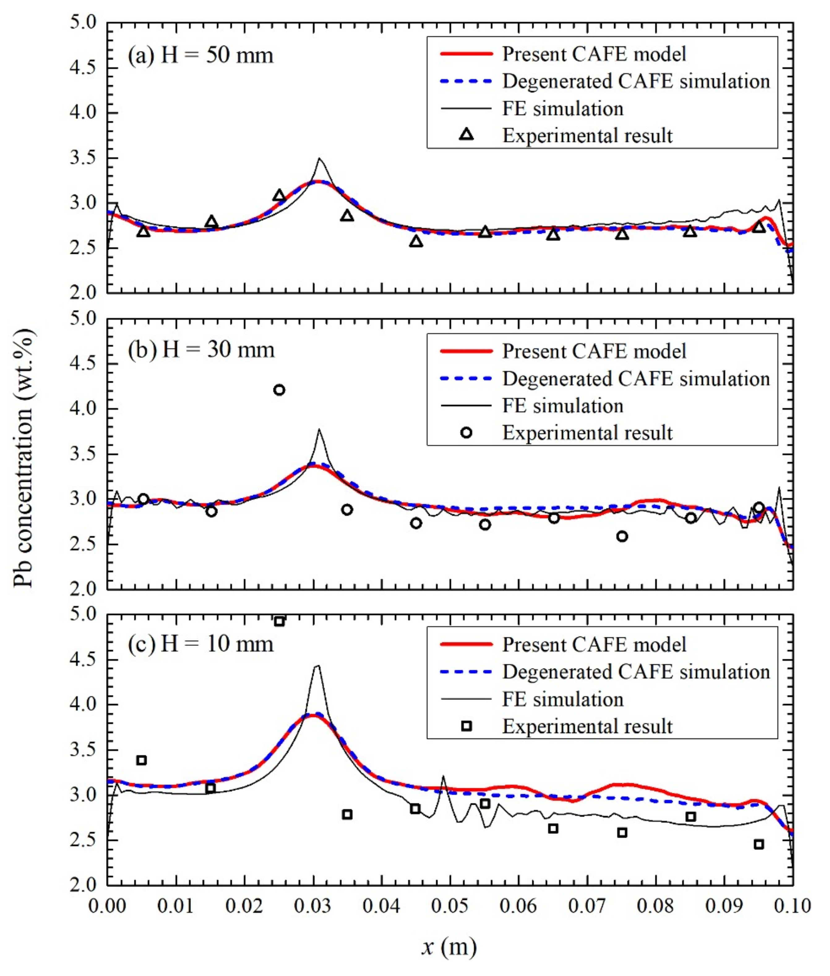
More quantitatively, Figure 11 presents comparisons of the final average mass concentration of Pb obtained by the above three simulations with the experimental measurements reported by Boussaa et al. [22] along the three horizontal lines L1–L3 (Figure 2) at the heights of 10 mm, 30 mm, and 50 mm in the ingots. A quite similar trend is shown between the simulated profiles and experimental measurements. However, the peaks corresponding to the plumes predicted by the three simulations are all smaller than their counterparts given by the experimental measurements, indicating an underestimated positive segregation. Furthermore, the same position of the peaks, x = 0.031 m, is predicted in all the three simulations, while the position of the peaks given by experimental measurements is about x = 0.025 m. Those differences may be caused by the simplified parameters for physical properties on one hand. On the other hand, model limitations, such as 2D approximation, isotropic permeability of the mushy zone, motionless equiaxed grains, and the neglected deformation and shrinkage, should also be responsible for those differences. Finally, it is of interest to underline that the profiles of Pb concentration predicted by the present CAFE model and the degenerated CAFE simulation also show obvious discrepancies in the right of the plume, though a good consistency is shown in the left of the plume.
4. Conclusions
A two-dimensional (2D) cellular automaton (CA)–finite element (FE) model has been developed to achieve a direct macroscopic modeling of grain structure and macrosegregation during the solidification of binary alloys. It consists of a macroscopic FE model that solves conservation equations averaged over a representative elementary volume based on an FE grid, a microscopic CA model that describes the evolution of the grain structure based on a CA grid, and a two-way coupling algorithm between the two models. The fluid flow is not only considered in the solution of macroscopic conservation equations, but also incorporated into the dendrite tip growth kinetics directly. The CAFE model is applied to a quasi-2D benchmark solidification experiment of a Sn–3.0wt.%Pb alloy, and the grain structure and macrosegregation are predicted simultaneously. It has been demonstrated that the present CAFE model has a capacity to consider the undercooling ahead of the growth front, which cannot be achieved by a purely macroscopic FE model with equilibrium solidification. Due to the instability of the growth front, both the isotherms and the solid fraction isolines are less smooth. Furthermore, a strong interaction between the fluid flow and grain structure is found. The growth directions of the columnar grains, grain sizes, and columnar-to-equiaxed transition (CET) position are obviously modified. In addition, the segregation maps obtained by the present CAFE model are quantitatively different from those given by a purely macroscopic FE model without consideration of the undercooling, and obvious segregated channels almost aligned with the orientations of the columnar grains are predicted.
It is believed that the present CAFE model gives a more reasonable prediction with profound principle. A qualitatively good agreement is obtained between the segregation profiles given by the present CAFE model and the experimental results. The quantitative differences may be attributed to the simplified parameters for physical properties to a great extent. Besides, model limitations, such as the 2D approximation, the isotropic permeability of the mushy zone, motionless equiaxed grains, and the neglected deformation and shrinkage, may also be to blame. Thus, improvements are needed to remove those limitations in the future.
Author Contributions
Conceptualization, Q.C. and H.S.; methodology, Q.C. and H.S.; software, Q.C.; validation, Q.C.; formal analysis, Q.C. and H.S.; investigation, Q.C. and H.S.; resources, H.S.; data curation, Q.C.; writing—original draft preparation, Q.C.; writing—review and editing, Q.C. and H.S.; visualization, Q.C. and H.S; supervision, H.S.; project administration, H.S.; funding acquisition, H.S.
Funding
This research was funded by the National Natural Science Foundation of China, grant number 51875307.
Conflicts of Interest
The authors declare no conflict of interest.
References
- Saito, Y.; Goldbeckwood, G.; Mullerkrumbhaar, H. Numerical simulation of dendritic growth. Phys. Rev. A 1988, 38, 2148–2157. [Google Scholar] [CrossRef] [Green Version]
- Boettinger, W.J.; Warren, J.A.; Beckermann, C.; Karma, A. Phase-field simulation of solidification. Annu. Rev. Mater. Res. 2002, 32, 163–194. [Google Scholar] [CrossRef]
- Steinbach, I. Phase-field models in materials science. Model. Simul. Mater. Sc. 2009, 17, 073001. [Google Scholar] [CrossRef] [Green Version]
- Gandin, C.A.; Rappaz, M. A coupled finite-element cellular-automaton model for the prediction of dendritic grain structures in solidfication processes. Acta Mater. 1994, 42, 2233–2246. [Google Scholar] [CrossRef]
- Xu, Q.Y.; Yang, C.; Zhang, H.; Yan, X.W.; Tang, N.; Liu, B.C. Multiscale Modeling and Simulation of Directional Solidification Process of Ni-Based Superalloy Turbine Blade Casting. Metals 2018, 8, 632. [Google Scholar] [CrossRef]
- Jacot, A.; Rappaz, M. A pseudo-front tracking technique for the modelling of solidification microstructures in multi-component alloys. Acta Mater. 2002, 50, 1909–1926. [Google Scholar] [CrossRef]
- Wang, W.; Lee, P.D.; McLean, M. A model of solidification microstructures in nickel-based superalloys: Predicting primary dendrite spacing selection. Acta Mater. 2003, 51, 2971–2987. [Google Scholar] [CrossRef]
- Tan, L.J.; Zabaras, N. A level set simulation of dendritic solidification with combined features of front-tracking and fixed-domain methods. J. Comput. Phys. 2006, 211, 36–63. [Google Scholar] [CrossRef] [Green Version]
- Wang, C.Y.; Beckermann, C. A unified solute diffusion-model for columnar and equiaxed dendritic alloy solidification. Mater. Sci. Eng. A 1993, 171, 199–211. [Google Scholar] [CrossRef]
- Wang, C.Y.; Beckermann, C. A multiphase solute diffusion-model for dendritic alloy solidification. Metall. Trans. A 1993, 24, 2787–2802. [Google Scholar] [CrossRef]
- Wang, C.Y.; Beckermann, C. Equiaxed dendritic solidification with convection. 1. Multiscale/multiphase modeling. Metall. Mater. Trans. A 1996, 27, 2754–2764. [Google Scholar] [CrossRef]
- Ciobanas, A.I.; Fautrelle, Y. Ensemble averaged multiphase Eulerian model for columnar/equiaxed solidification of a binary alloy: I. The mathematical model. J. Phys. D 2007, 40, 3733–3762. [Google Scholar] [CrossRef]
- Appolaire, B.; Combeau, H.; Lesoult, G. Modeling of equiaxed growth in multicomponent alloys accounting for convection and for the globular/dendritic morphological transition. Mater. Sci. Eng. A 2008, 487, 33–45. [Google Scholar] [CrossRef]
- Wu, M.; Ludwig, A. Modeling equiaxed solidification with melt convection and grain sedimentation-I: Model description. Acta Mater. 2009, 57, 5621–5631. [Google Scholar] [CrossRef]
- Schneider, M.C.; Beckermann, C. Formation of macrosegregation by multicomponent thermosolutal convection during the solidification of steel. Metall. Mater. Trans. A 1995, 26, 2373–2388. [Google Scholar] [CrossRef]
- Guillemot, G.; Gandin, C.A.; Combeau, H. Modeling of macrosegregation and solidification grain structures with a coupled Cellular Automaton-Finite Element model. ISIJ Int. 2006, 46, 880–895. [Google Scholar] [CrossRef]
- Gandin, C.A.; Guillemot, G.; Bellet, M. Interaction between single grain solidification and macrosegregation: Application of a cellular automaton-Finite element model. J. Cryst. Growth 2007, 303, 58–68. [Google Scholar]
- Carozzani, T.; Gandin, C.A.; Digonnet, H.; Bellet, M.; Zaidat, K.; Fautrelle, Y. Direct Simulation of a Solidification Benchmark Experiment. Metall. Mater. Trans. A 2013, 44, 873–887. [Google Scholar] [CrossRef]
- Quillet, G.; Ciobanas, A.; Lehmann, P.; Fautrelle, Y. A benchmark solidification experiment on an Sn-10 wt%Bi alloy. Int. J. Heat Mass Transf. 2007, 50, 654–666. [Google Scholar] [CrossRef]
- Hachani, L.; Saadi, B.; Wang, X.D.; Nouri, A.; Zaidat, K.; Belgacem-Bouzida, A.; Ayouni-Derouiche, L.; Raimondi, G.; Fautrelle, Y. Experimental analysis of the solidification of Sn-3 wt.%Pb alloy under natural convection. Int. J. Heat Mass Transf. 2012, 55, 1986–1996. [Google Scholar] [CrossRef]
- Hachani, L.; Zaidat, K.; Saadi, B.; Wang, X.D.; Fautrelle, Y. Solidification of Sn-Pb alloys: Experiments on the influence of the initial concentration. Int. J. Therm. Sci. 2015, 91, 34–48. [Google Scholar] [CrossRef]
- Boussaa, R.; Hachani, L.; Budenkova, O.; Botton, V.; Henry, D.; Zaidat, K.; Ben Hadid, H.; Fautrelle, Y. Macrosegregations in Sn-3 wt%Pb alloy solidification: Experimental and 3D numerical simulation investigations. Int. J. Heat Mass Transf. 2016, 100, 680–690. [Google Scholar] [CrossRef]
- Chen, Q.P.; Shen, H.F. A finite element formulation for macrosegregation during alloy solidification using a fractional step method and equal-order elements. Comp. Mater. Sci. 2018, 154, 335–345. [Google Scholar] [CrossRef]
- Yeh, C.; Chang, L.; Straumal, B. Wetting transition of grain boundaries in tin-rich indium-based alloys and its influence on electrical properties. Mater. Trans. 2010, 51, 1677–1682. [Google Scholar] [CrossRef]
- Straumal, B.B.; Kogtenkova, O.A.; Muktepavela, F.; Kolesnikova, K.I.; Bulatov, M.F.; Straumal, P.B.; Baretzky, B. Direct observation of strain-induced non-equilibrium grain boundaries. Mater. Lett. 2015, 159, 432–435. [Google Scholar] [CrossRef]
- Bellet, M.; Combeau, H.; Fautrelle, Y.; Gobin, D.; Rady, M.; Arquis, E.; Budenkova, O.; Dussoubs, B.; Duterrail, Y.; Kumar, A.; et al. Call for contributions to a numerical benchmark problem for 2D columnar solidification of binary alloys. Int. J. Therm. Sci. 2009, 48, 2013–2016. [Google Scholar] [CrossRef]
- Thevoz, P.; Desbiolles, J.L.; Rappaz, M. Modeling of equiaxed microstructure formation in casting. Metall. Trans. A 1989, 20, 311–322. [Google Scholar] [CrossRef]
- Rappaz, M.; Gandin, C.A. Probabilistic modeling of microstructure formation in solidification processes. Acta Mater. 1993, 41, 345–360. [Google Scholar] [CrossRef]
- Gandin, C.A.; Guillemot, G.; Appolaire, B.; Niane, N.T. Boundary layer correlation for dendrite tip growth with fluid flow. Mater. Sci. Eng. A 2003, 342, 44–50. [Google Scholar] [CrossRef]
- Lipton, J.; Glicksman, M.E.; Kurz, W. Dendritic growth into undercooled alloy melts. Mater. Sci. Eng. 1984, 65, 57–63. [Google Scholar] [CrossRef]
- Gandin, C.A.; Desbiolles, J.L.; Rappaz, M.; Thevoz, P. A three-dimensional cellular automaton-finite element model for the prediction of solidification grain structures. Metall. Mater. Trans. A 1999, 30, 3153–3165. [Google Scholar] [CrossRef]
- Ananth, R.; Gill, W.N. Self-consistent theory of dendritic growth with convection. J. Cryst. Growth 1991, 108, 173–189. [Google Scholar] [CrossRef]
Figure 1.
Schematic of different length scales included in the present CAFE model: (a) macroscopic FE grid of triangular elements, (b) microscopic CA grid of square cells, and (c) grain envelope described in each cell.
Figure 1.
Schematic of different length scales included in the present CAFE model: (a) macroscopic FE grid of triangular elements, (b) microscopic CA grid of square cells, and (c) grain envelope described in each cell.

Figure 2.
Schematic of the solidification configuration of a Sn–3wt.%Pb ingot. The coordinates of locations P1–P4 are expressed in millimeters.
Figure 2.
Schematic of the solidification configuration of a Sn–3wt.%Pb ingot. The coordinates of locations P1–P4 are expressed in millimeters.
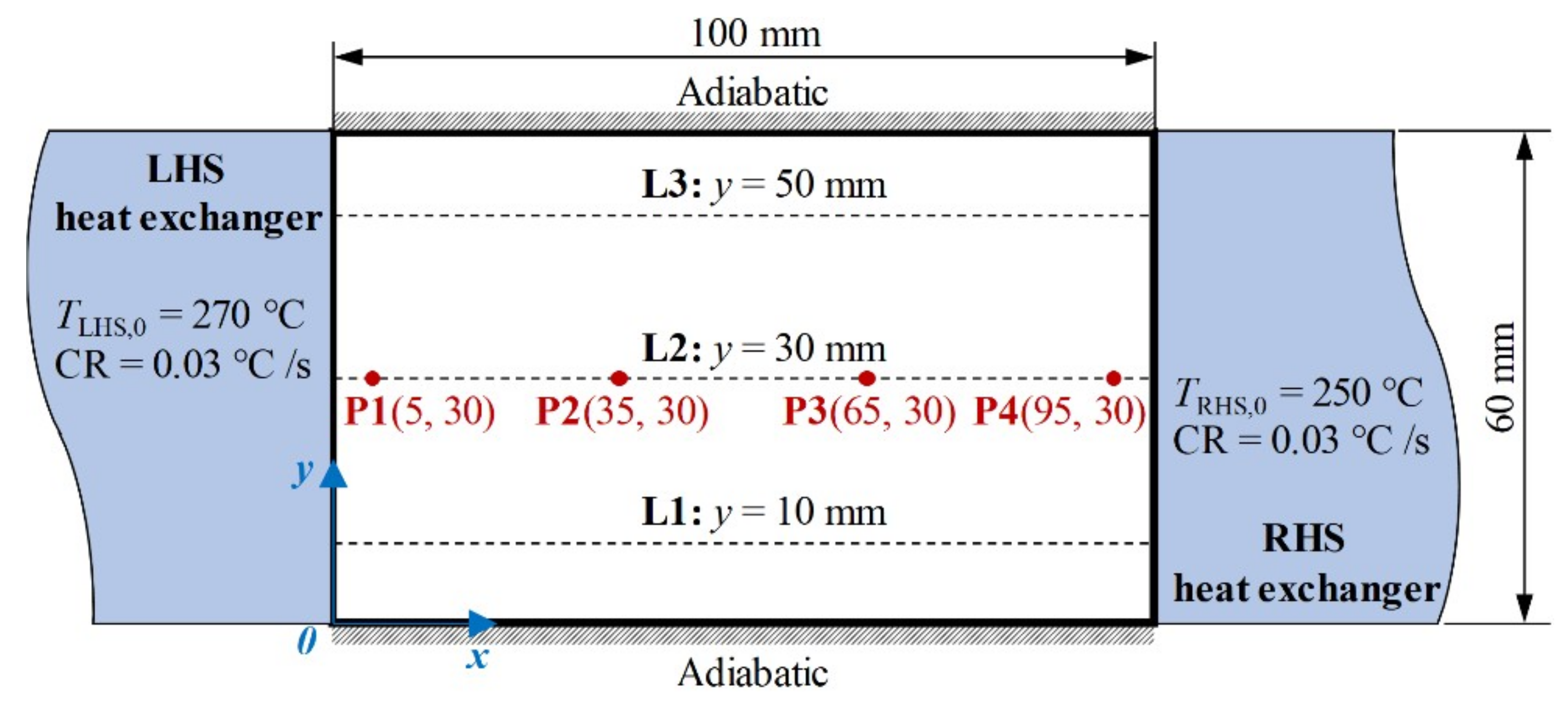
Figure 3.
Variations of the dendrite tip growth velocity of Sn–Pb alloys with the Pb composition for different values of the undercooling in the presence of fluid flow (, ).
Figure 3.
Variations of the dendrite tip growth velocity of Sn–Pb alloys with the Pb composition for different values of the undercooling in the presence of fluid flow (, ).
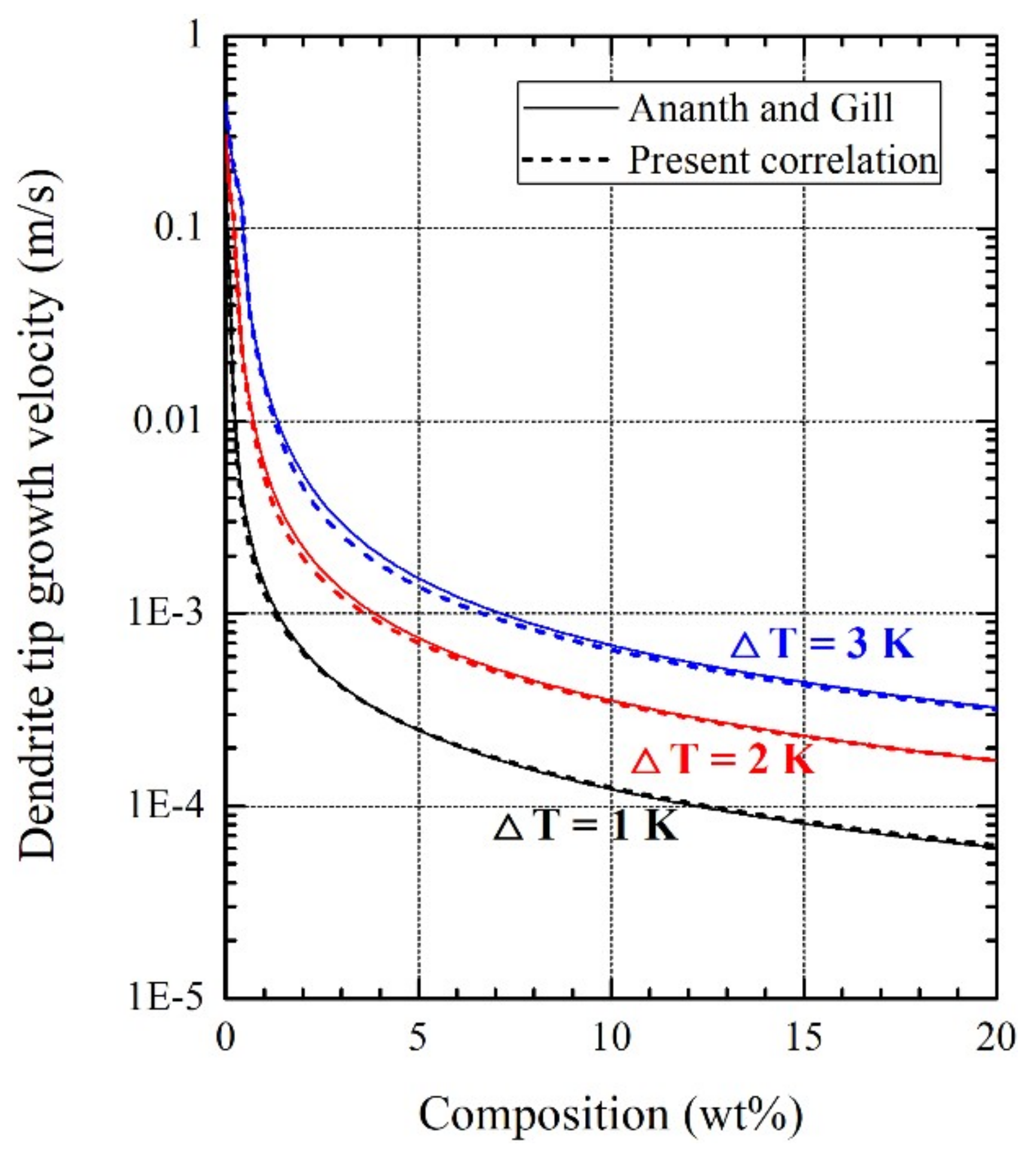
Figure 4.
Variations of the dendrite tip growth velocity of Sn–3wt%Pb alloy with the undercooling for different values of the fluid flow velocity ().
Figure 4.
Variations of the dendrite tip growth velocity of Sn–3wt%Pb alloy with the undercooling for different values of the fluid flow velocity ().
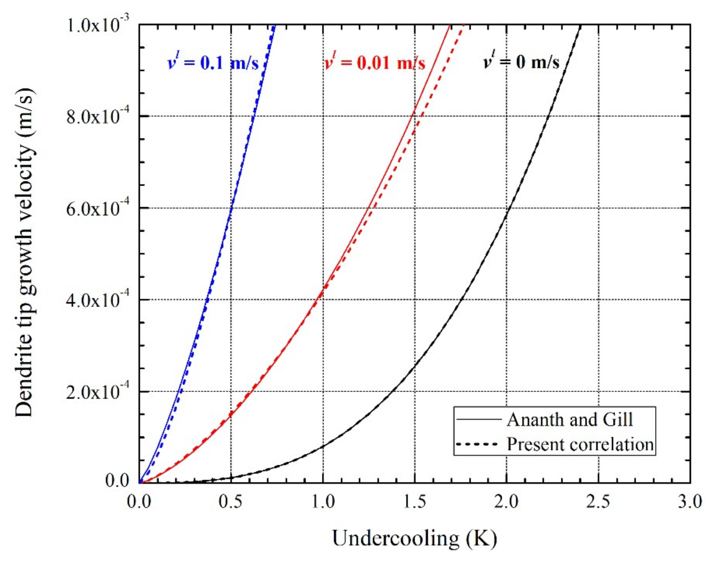
Figure 5.
Polar plot of the dendrite tip growth velocity of Sn–3wt%Pb alloy with K as a function of the angle between the preferential orientations and the liquid velocity vector in the presence and absence of fluid flow.
Figure 5.
Polar plot of the dendrite tip growth velocity of Sn–3wt%Pb alloy with K as a function of the angle between the preferential orientations and the liquid velocity vector in the presence and absence of fluid flow.
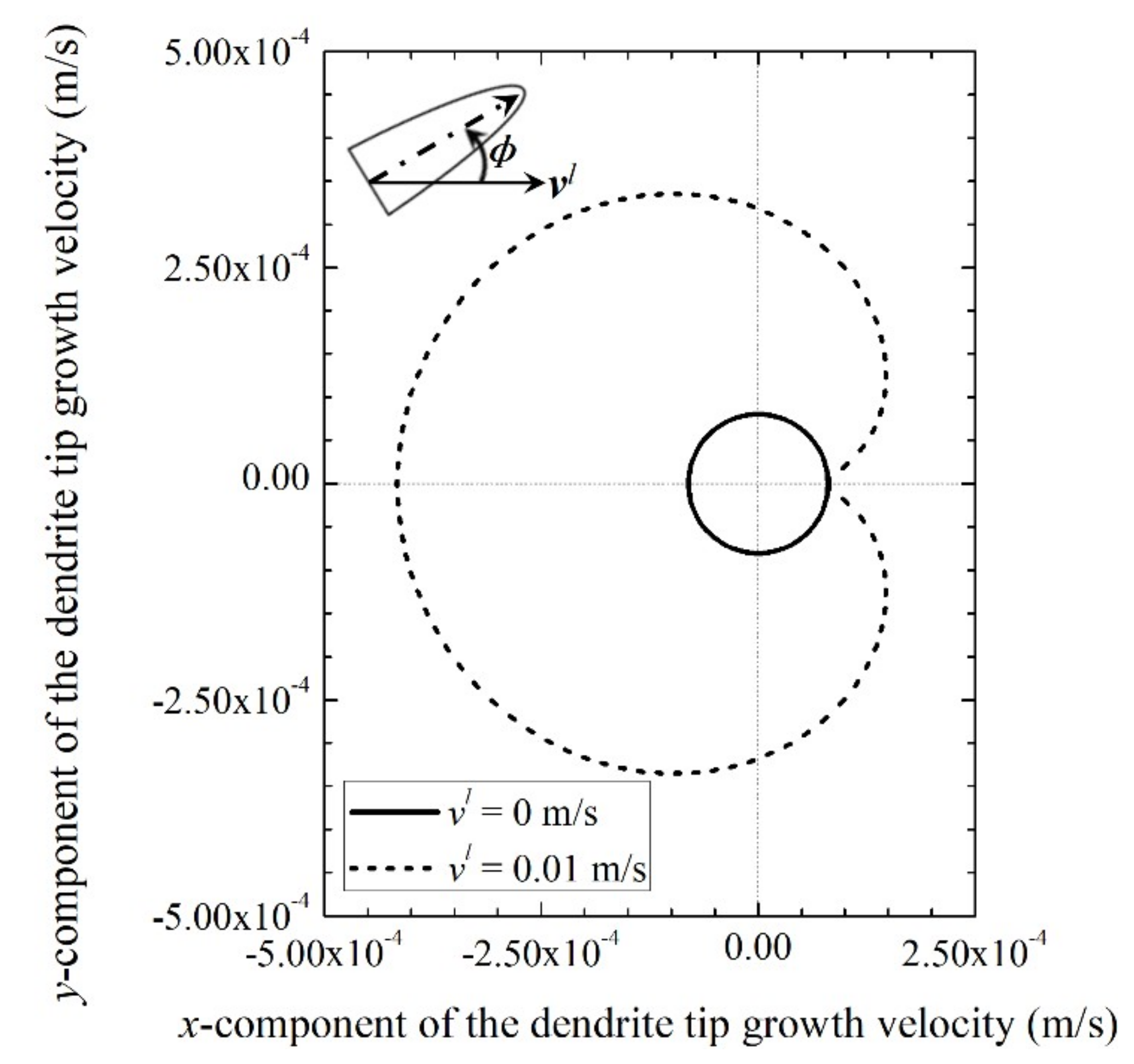
Figure 6.
Temperature fields predicted at selected instants during solidification of the Sn–3wt.%Pb ingot: (a) 1000 s, (b) 1750 s, (c) 2000 s, (d) 2300 s, (e) 2500 s, and (f) 2700 s.
Figure 6.
Temperature fields predicted at selected instants during solidification of the Sn–3wt.%Pb ingot: (a) 1000 s, (b) 1750 s, (c) 2000 s, (d) 2300 s, (e) 2500 s, and (f) 2700 s.
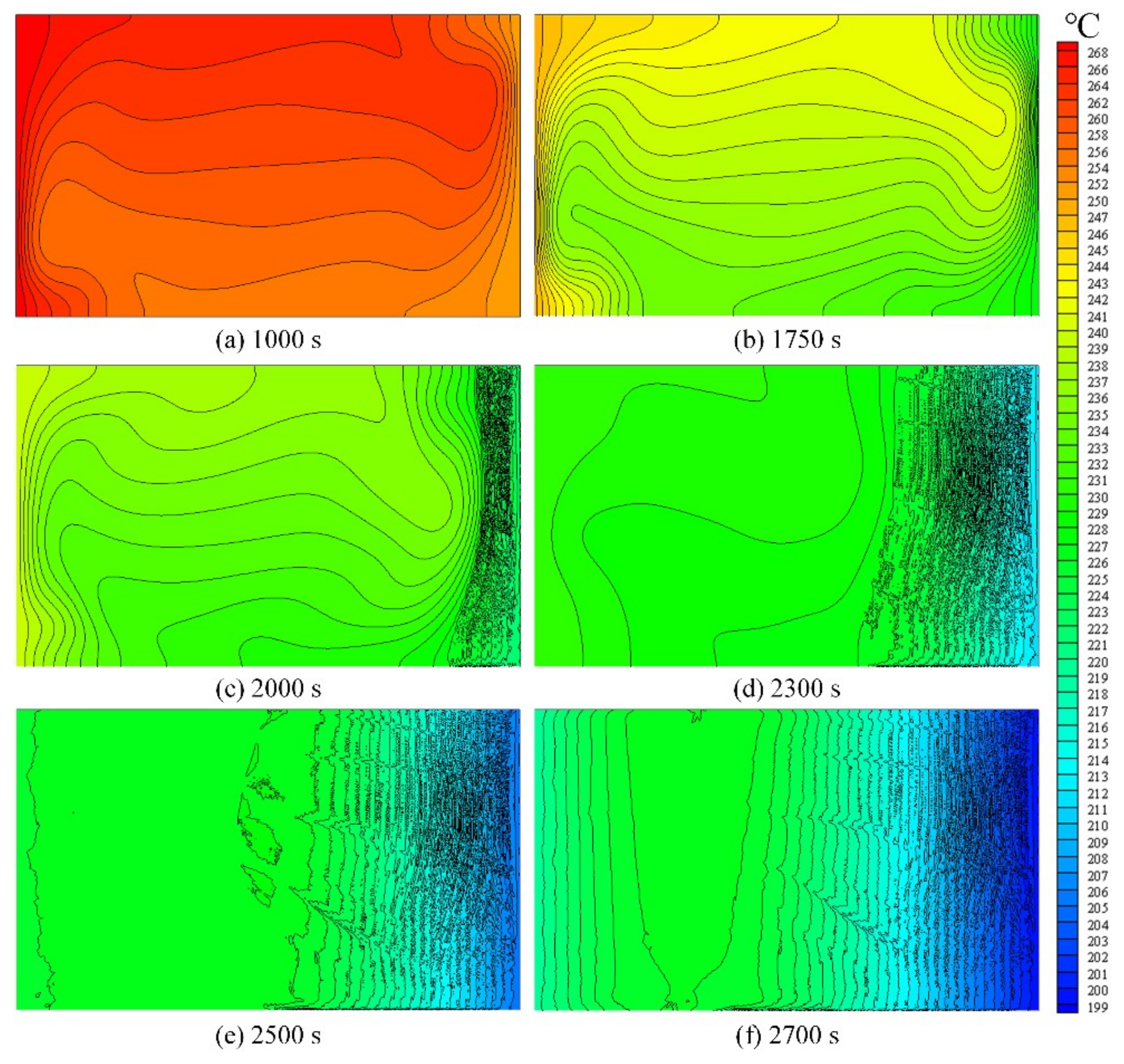
Figure 7.
Solid fraction fields predicted at selected instants during solidification of the Sn–3wt.%Pb alloy: (a) 2000 s, (b) 2300 s, (c) 2500 s, and (d) 2700 s. The white and red profiles correspond to the solid fraction of 0.0001 predicted by the present CAFE model and a purely macroscopic FE simulation disabling the CA model (equilibrium solidification), respectively.
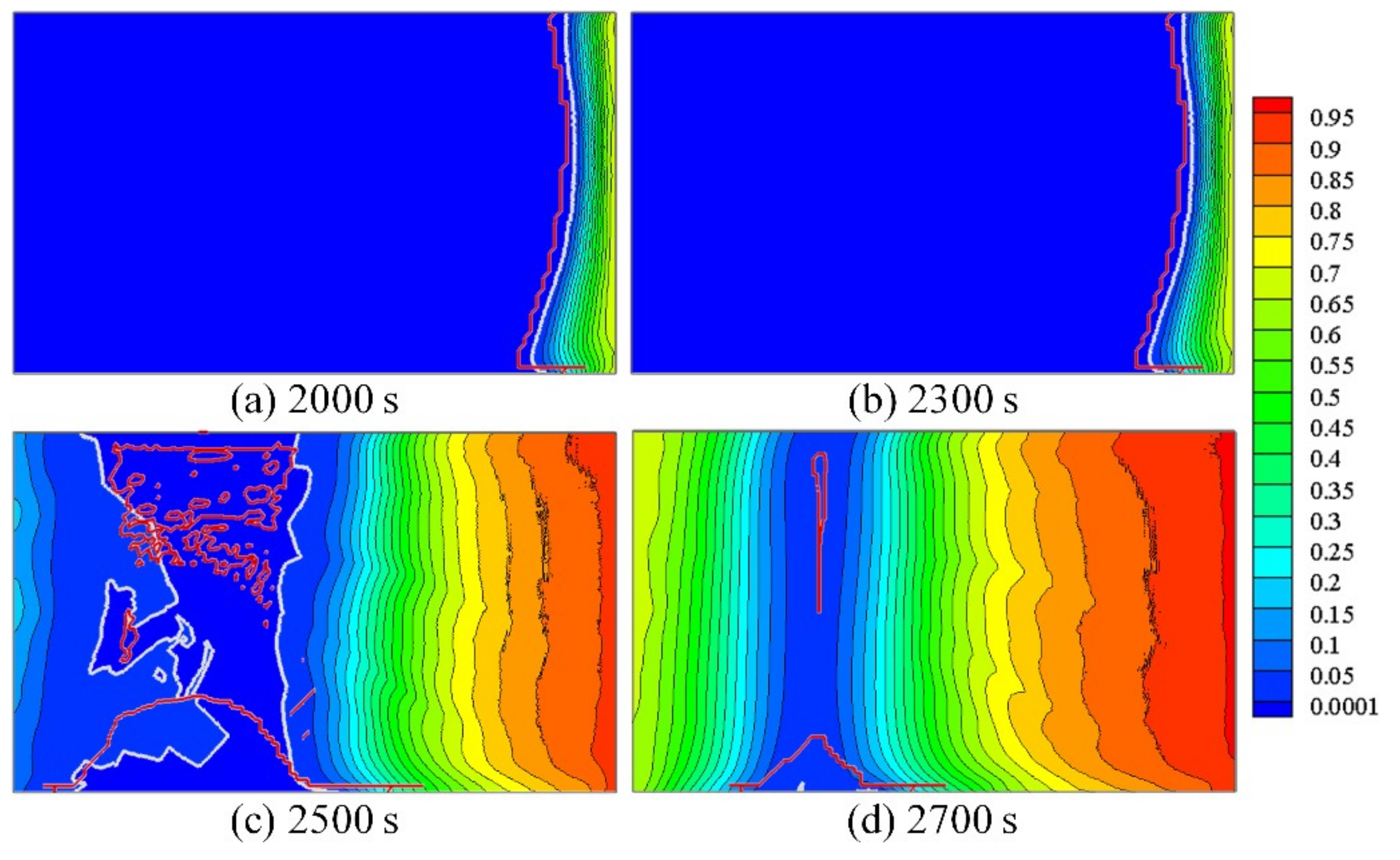
Figure 8.
Comparisons of the cooling curves and the solid fraction evolutions obtained by the present CAFE model and a purely macroscopic FE simulation disabling the CA model at the four locations P1–P4 of the Sn–3wt.%Pb ingot.
Figure 8.
Comparisons of the cooling curves and the solid fraction evolutions obtained by the present CAFE model and a purely macroscopic FE simulation disabling the CA model at the four locations P1–P4 of the Sn–3wt.%Pb ingot.
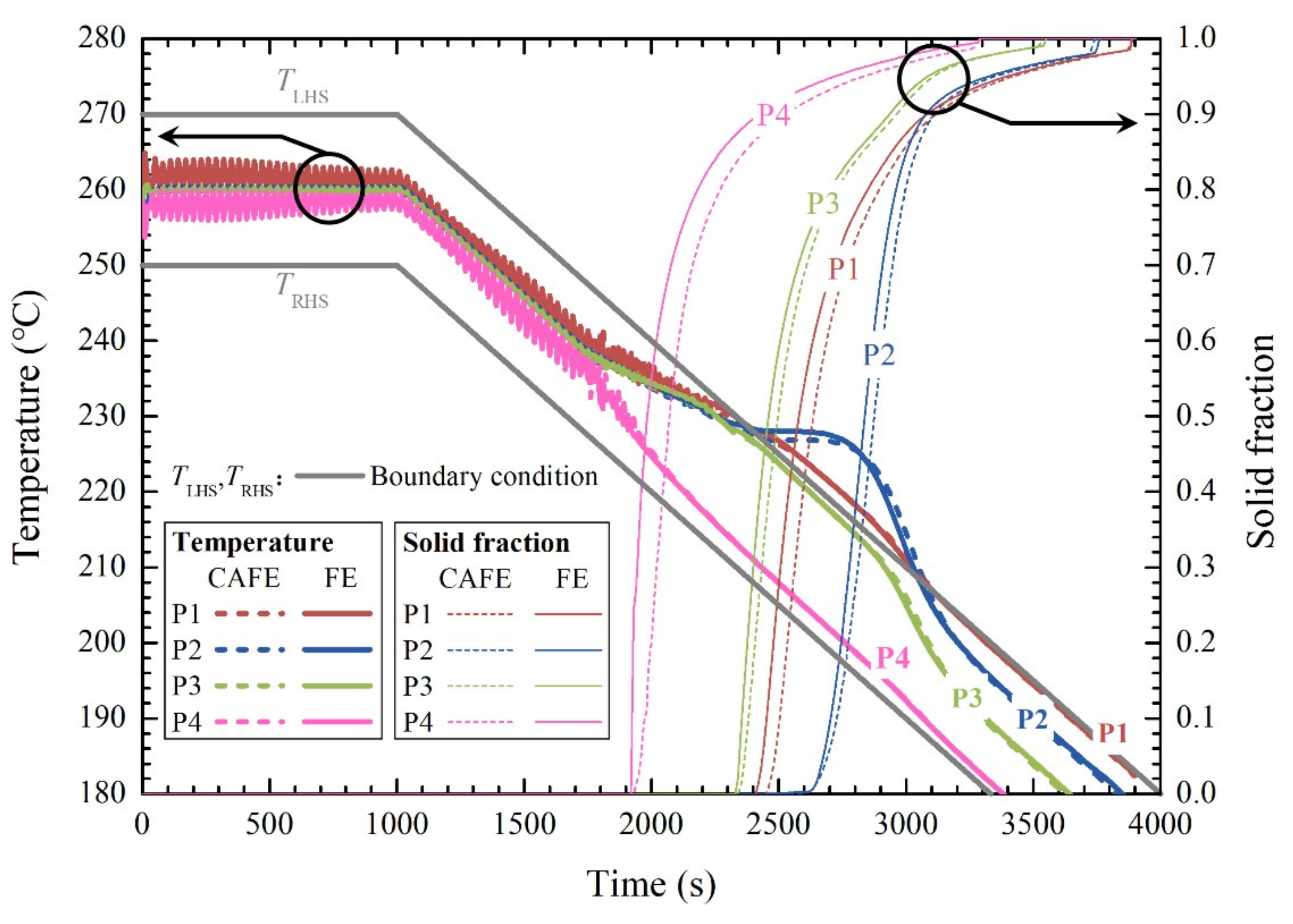
Figure 9.
Comparisons of the grain structure and the fluid flow at selected instants during solidification of the Sn–3wt.%Pb alloy. Figure (a1–d1) and figure (a2–d2) are obtained by the present CAFE model and a degenerated CAFE simulation disabling the effect of the fluid flow on dendrite tip growth kinetics, respectively.
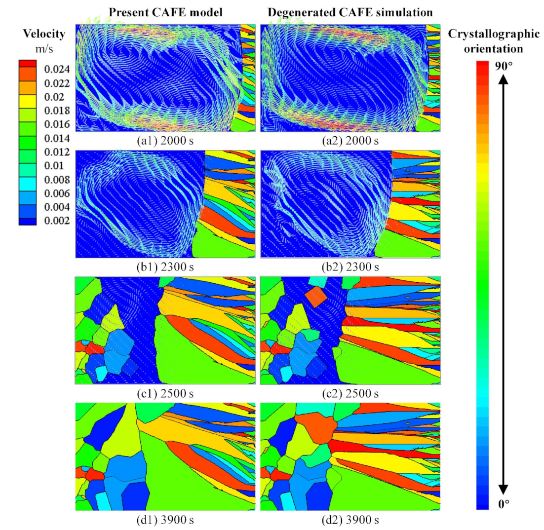
Figure 10.
Comparisons of the segregation maps obtained by the present CAFE model (a1–d1), a degenerated CAFE simulation disabling the effect of the fluid flow on the dendrite tip growth kinetics (a2–d2), and a purely macroscopic FE simulation disabling the CA model (a3–d3) at selected instants during solidification of the Sn–3wt.%Pb alloy.
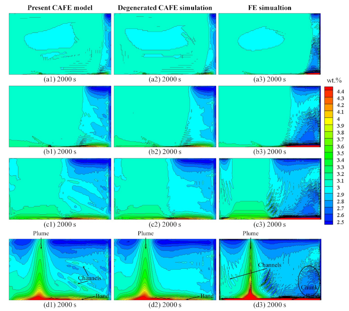
Figure 11.
Comparisons of the final average mass concentration of Pb obtained by the present CAFE model, a degenerated CAFE simulation disabling the effect of the fluid flow on the dendrite tip growth kinetics, and a purely macroscopic FE simulation disabling the CA model with the experimental measurements [22] along the three horizontal lines L1–L3 at the heights of 10 mm, 30 mm, and 50 mm in the ingots (Figure 2).

| Parameter Description | Symbol | Value | Unit |
|---|---|---|---|
| Phase diagram | |||
| Melting temperature | 232.0 | °C | |
| Eutectic temperature | 183.0 | °C | |
| Eutectic composition | 38.1 | wt.% | |
| Partition coefficient | 0.0656 | - | |
| Physical properties | |||
| Reference density | 7130.0 | kg·m−3 | |
| Solutal expansion coefficient | −5.3 × 10⁻³ | wt.%−1 | |
| Thermal expansion coefficient | 9.5 × 10⁻⁵ | K−1 | |
| Specific heat of the liquid | 265.0 | J·kg−1·K−1 | |
| Specific heat of the solid | 226.0 | J·kg−1·K−1 | |
| Latent heat | 57,512.0 | J·kg−1 | |
| Thermal conductivity of the liquid | 55.0 | W·m−1·K−1 | |
| Thermal conductivity of the solid | 33.0 | W·m−1·K−1 | |
| Diffusion coefficient of Pb in liquid Sn | 3.0 × 10⁻⁹ | m2·s−1 | |
| Dynamic viscosity of the liquid | 2.0 × 10⁻³ | Pa·s | |
| Initial and boundary conditions | |||
| Nominal composition | 3.0 | wt.% | |
| Initial temperature | 258.6 | °C | |
| Initial velocity | 0 | m·s−1 | |
| Initial temperature of the LHS wall | 270.0 | °C | |
| Initial temperature of the RHS wall | 250.0 | °C | |
| Cooling rate on the LHS and RHS walls | −0.03 | °C·s−1 | |
| Nucleation and grain growth | |||
| Gibbs–Thomson coefficient | 2.0 × 10⁻⁷ | m·K | |
| Gaussian distribution nucleation parameters on the RHS wall | |||
| Average undercooling | 1.0 | K | |
| Standard deviation | 0.5 | K | |
| Density of nucleation sites | 1.0 × 10⁶ | m−2 | |
| Gaussian distribution nucleation parameters in the bulk melt | |||
| Average undercooling | 2.5 | K | |
| Standard deviation | 0.5 | K | |
| Density of nucleation sites | 1.0 × 10⁸ | m−3 | |
| Additional parameters | |||
| FE mesh size | 1.0 × 10⁻³ | m | |
| FE time step | 0.05 | s | |
| CA cell size | 2.0 × 10⁻⁴ | m | |
© 2019 by the authors. Licensee MDPI, Basel, Switzerland. This article is an open access article distributed under the terms and conditions of the Creative Commons Attribution (CC BY) license (http://creativecommons.org/licenses/by/4.0/).
Share and Cite
MDPI and ACS Style
Chen, Q.; Shen, H. Direct Macroscopic Modeling of Grain Structure and Macrosegregation with a Cellular Automaton–Finite Element Model. Metals 2019, 9, 177. https://doi.org/10.3390/met9020177
AMA Style
Chen Q, Shen H. Direct Macroscopic Modeling of Grain Structure and Macrosegregation with a Cellular Automaton–Finite Element Model. Metals. 2019; 9(2):177. https://doi.org/10.3390/met9020177
Chicago/Turabian StyleChen, Qipeng, and Houfa Shen. 2019. "Direct Macroscopic Modeling of Grain Structure and Macrosegregation with a Cellular Automaton–Finite Element Model" Metals 9, no. 2: 177. https://doi.org/10.3390/met9020177
Note that from the first issue of 2016, this journal uses article numbers instead of page numbers. See further details here.