Prediction of Central Carbon Segregation in Continuous Casting Billet Using A Regularized Extreme Learning Machine Model

Abstract

Central carbon segregation is a typical internal defect of continuous cast steel billets. Real-time and accurate carbon segregation prediction is of great significance for lean control of the production quality in continuous casting processes. In this paper, a data-driven regularized extreme learning machine (R-ELM) model is proposed for the prediction of carbon segregation index (CSI). To improve model performance, outliers in industrial data were eliminated by means of boxplot tool. Besides, Pearson correlation combined with grey relational analysis (GRA) was conducted to avoid multicollinearity and redundancy in input variables. The new model shows potential to evaluate online quality of steel billets. When predictive errors were within ±0.03 and ±0.025, the prediction accuracy of the R-ELM model was 94% and 89%, respectively, which was higher than that of the multiple linear regression (MLR) model and ELM model. Moreover, the effects of several key continuous casting process parameters on CSI were investigated based on the predictions of the R-ELM model via response surface analysis. The conclusions are consistent with the metallurgical mechanism, and the predictive values of the R-ELM model agree well with experimental values, which further verifies the correctness and generalization ability of the R-ELM model.

1. Introduction

In order to reduce production cost and improve product competitiveness in the continuous casting process of steel, technologies have been developing rapidly, such as continuous casting hot charging and continuous casting direct rolling [1,2]. A compact and efficient production mode has become the pursuit of continuous casting production. Apparently, traditional quality evaluation methods have been unable to meet the needs of modern steel plants, and there is no chance to check the steel billets off-line through artificial sampling due to its compact and continuous production characteristics. In this setting, effective online prediction models of quality defects are urgently needed to guide the actual production.

Central carbon segregation is a common internal defect of continuous cast steel billets, leading to non-uniformity in the mechanical properties of the final products, which can hardly be alleviated by the subsequent heat treatment and rolling processes [3]. The formation of central carbon segregation is an intrinsic feature of the solidification process, since the dissolved elements generally have a higher solubility in the liquid phase than in the solid [4]. As the solidification time goes on, a part of the solute-rich material is trapped between the primary dendritic arms, which leads to micro-segregation; while the other part is pushed out to the centerline or the channels formed by solidification shrinkage within the equiaxed zone. The latter effects give rise to centerline and ‘V’ type segregates. The factors affecting center segregation are well known, such as superheat, secondary cooling, casting speed, steel chemistry, etc. Electromagnetic stirring and soft reduction are important measures to suppress center segregation. Electromagnetic stirring can promote the flow of molten steel, not only reducing the superheat of steel, but also breaking the dendrites and promoting the formation of a crystal nucleus. Soft reduction can offset the solidification shrinkage in the two-phase zone of steel by squeezing the billet at the solidification end, which thus encourages the redistribution of solute-rich material. Electromagnetic stirring combined with soft reduction is a common method to suppress central segregation in the continuous casting process of steel.

It is nearly impossible to completely eliminate the carbon segregation in the continuous casting process, but attempts have been made to predict and control it. Due to the complex physical phenomena during the continuous casting process of steel, the quantitative prediction of carbon segregation is extremely difficult [5]. Currently, the evaluation methods of central carbon segregation mainly include those based on metallurgical mechanism and artificial intelligence (AI) methods. The metallurgical mechanism methods involve establishing the functional relationship between process parameters and central carbon segregation, and determining the segregation level. Many scholars have made contributions in this aspect especially by means of numerical simulation [6,7,8,9]. Numerical models are powerful tools which are capable of capturing the overall segregation evolution with good visualization. Nevertheless, the complex model architecture and the unacceptable computational efforts have become the bottleneck restricting the online use of the numerical models.

In recent years, artificial intelligence technology has been developing rapidly in material property prediction because of its advantages in dealing with highly complex problems. However, the artificial intelligence technology was rarely used to predict the central carbon segregation in steel billets. García et al. [10] built a segregation prediction model of slab based on multivariate adaptive regression splines technique, and the results showed good agreement with the actual values. Besides, to predict the centerline segregation in continuous cast steel slabs, a hybrid algorithm was established based on support vector machine in combination with the particle swarm optimization algorithm [11]. Normanton et al. [12] developed a quality prediction system of steel casting, which was a combination of several artificial intelligence techniques, such as artificial neural networks, multi-layer perceptron nets, and self-organizing maps and other database methods. The system was trialed successfully on plants. Extreme learning machine (ELM) has drawn increasing attention among scholars from various fields due to its high learning efficiency and strong generalization ability in recent years. Chen et al. [13] achieved the accurate prediction for central carbon segregation of slabs based on ELM algorithm, and the calculation time was only 0.1 s. Although the above models can provide valuable guidance for actual production, their generalization ability cannot be guaranteed due to the lack of sufficient data preprocessing efforts.

In view of the difficulty of quantitative prediction for central carbon segregation, this paper maximizes the value of historical industrial data through data preprocessing efforts, and attempts are made to achieve accurate prediction for central carbon segregation based on an improved regularized ELM (R-ELM) model. The workflow of this study is shown in Figure 1. The background and experimental data are introduced first. Furthermore, data cleaning and feature engineering are carried out for the data collected from one steelmaking plant. Based on these, a multiple linear regression (MLR) model, ELM model, and R-ELM model are established, respectively, for central carbon segregation prediction. After that, the optimal model is chosen by comparing their prediction accuracy. Finally, the correctness and generalization ability of the optimal model are further verified.

2. Problem Description and Experimental Data

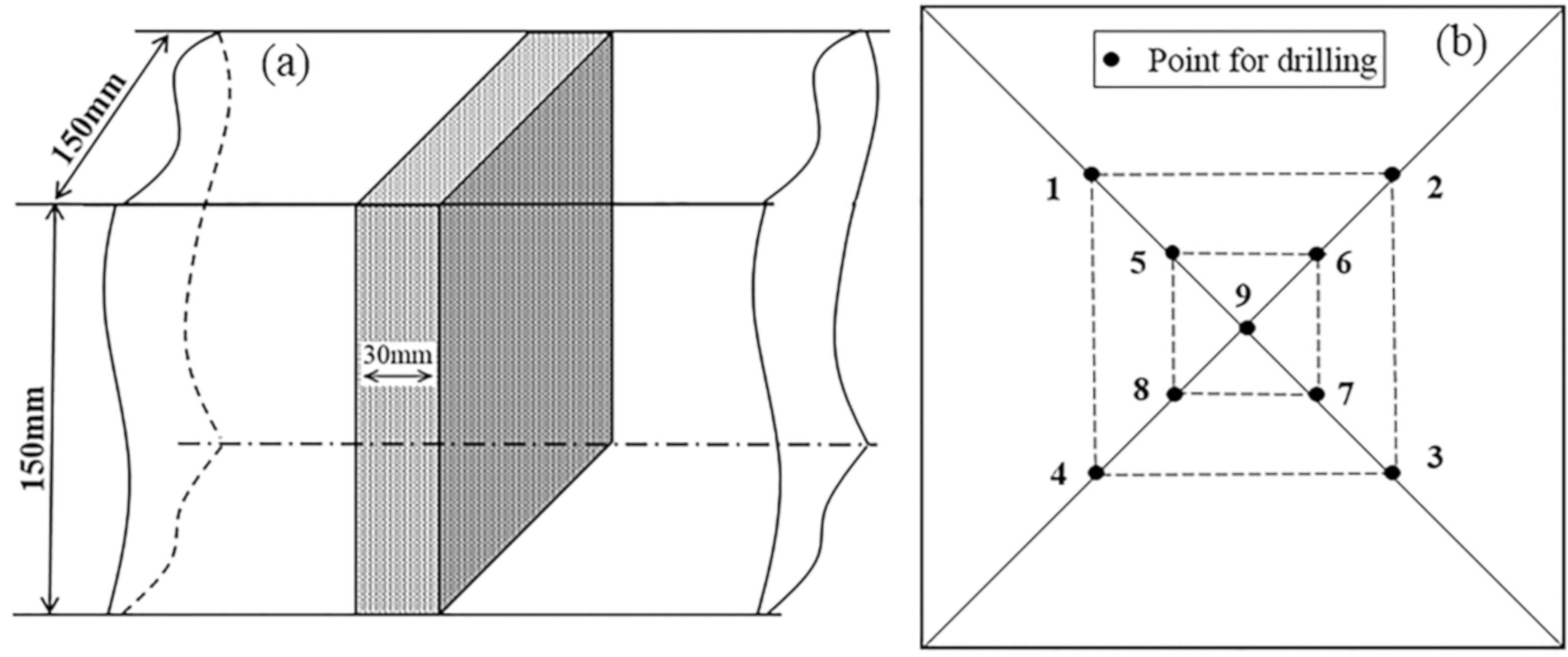
2.1. Problem Description

Continuous casting is a complex production process in which high temperature molten steel is continuously cast into billets with a certain section shape and size. The transformation from molten steel to billets is accompanied by a series of complex phenomena, such as flow, solidification, mass transfer, and heat transfer. The defect of central carbon segregation in continuous casting billets is formed under the complex interaction of the above factors. According to the production practice, a continuous casting process has the following characteristics: (1) numerous factors affecting central carbon segregation: including the chemical composition of molten steel, cooling parameters of the mold zone and secondary cooling zones, electromagnetic stirring process, and other casting parameters, such as superheat and casting speed. (2) Strong coupling among factors: the interaction of various physical phenomena in a continuous casting process leads to the strong coupling among process parameters, which is difficult to explain by metallurgical mechanisms. (3) Information feedback of central carbon segregation is lagged: the quality estimation for carbon segregation is mostly based on off-line manual sampling and detection. The large lag of quality inspection and information feedback of central carbon segregation makes the process parameters unavailable to be adjusted in time and the production is difficult to be ensured. Therefore, in order to better assist continuous casting production, it is of great significance to use the model with strong approximation ability to predict carbon segregation. Therefore, prediction models based on machine learning can be suitable to solve this problem. The main idea of machine learning modeling involves establishing the complex mapping relationship between the continuous casting parameters (model inputs) and the carbon segregation indicator (model output) with the aid of historical production data, and realizing carbon segregation prediction.

2.2. Experimental Data

The data of high carbon steel C80D used for central carbon segregation prediction were collected from the production record of the caster belonging to Xiangtan Iron & Steel Co., Ltd of Hunan Valin (Xiangtan, China). The chemical compositions of high carbon steel C80D is shown in

Table 1. Chemical composition of C80D steel.

Composition	C	Si	Mn	P	S	Cr	Cu
Mass fraction, %	0.79~0.82	0.15~0.35	0.60~0.90	≤0.025	≤0.025	≤0.25	≤0.25

. This caster is a four-strand circular-arc caster that mainly produce billets with the section size of 150 mm × 150 mm. The dataset contains 2476 samples after deleting null and duplicate data, and each sample consists of 14 industrial parameter values and the corresponding carbon segregation index (CSI) value. As shown in

Table 2. Main continuous casting production parameters related to the carbon segregation index (CSI).

Symbols	Names of Production Parameters	Units
X1	Carbon content in molten steel	wt. %
X2	Silicon content in molten steel	wt. %
X3	Manganese content in molten steel	wt. %
X4	Phosphorus content in molten steel	wt. %
X5	Sulfur content in molten steel	wt. %
X6	Secondary cooling water flow rate in zone1	L/min
X7	Secondary cooling water flow rate in zone2	L/min
X8	Secondary cooling water flow rate in zone3	L/min
X9	Secondary cooling intensity	L/kg
X10	Pouring temperature	°C
X11	Casting speed	m/min
X12	Superheat	°C
X13	Mold water flow rate	L/min
X14	Mold water temperature difference	°C

, industrial parameters mainly involve chemical compositions of molten steel, as well as process and facility parameters related to central carbon segregation. Electromagnetic stirring is an important process to improve central carbon segregation. However, the parameters of stirring current and frequency are set to designated values in the continuous casting process, which is not taken into account. CSI is an important indicator used to characterize the level of central carbon segregation. Both longitudinal and cross-sectional observations have been commonly used to evaluate the central carbon segregation. The longitudinal methods are more effective to show the development and the distribution of segregation along the casting direction. However, the continuous casting process is fast paced, which allows insufficient time to conduct detailed evaluation. Thus, cross section drilling data were used in the current work, which can be obtained efficiently at a low cost. Figure 2 shows the schematic diagrams of sampling and drilling in a continuous casting steel billet. As shown in Figure 2a, samples with a cross section of 150 × 150 mm and thickness of 30 mm were cut off from the billets. After that, alloy drills with a diameter of 5 mm were used to drill steel chips at the 1/4, 1/2, and 1/8 lengths in diagonal lines of the billet cross section, as shown in Figure 2b. All the drillings were analyzed by a carbon-sulfur analyzer. Then, the CSI can be calculated using Equation (1).

$$CSI=9C_9/{\displaystyle \sum _{i=1}^9{C}_i}.$$

(1)

3. Data Cleaning

During the continuous casting process of steel, there are inevitably a small portion of abnormal data caused by the instability of the detection equipment and the misoperation of workers. The existence of abnormal data in the dataset largely influences the comprehensive performance of machine learning prediction models. Data cleaning is a crucial step of data preprocessing, which is to transform the noisy data into the data that meets the requirements of the prediction model. According to statistics, the data preprocessing stage takes 50% or even 80% of the overall data mining process effort [14,15].

3.1. Data Normalization

In order to weaken the influence of numerical difference of variables on the convergence speed of the machine learning model, the method of maximum and minimum normalized the data to the range of [−1,1]. The equation is shown as follows:

$$y=\frac{\left(y_{\max }-y_{\min }\right)\times \left(x-x_{\min }\right)}{\left(x_{\max }-x_{\min }\right)}+y_{\min },$$

(2)

where, y is the normalized value; x is the raw value; y_max and y_min are the maximum and minimum values within the mapping interval, respectively; x_max and x_min are the maximum and minimum values in each variable, respectively.

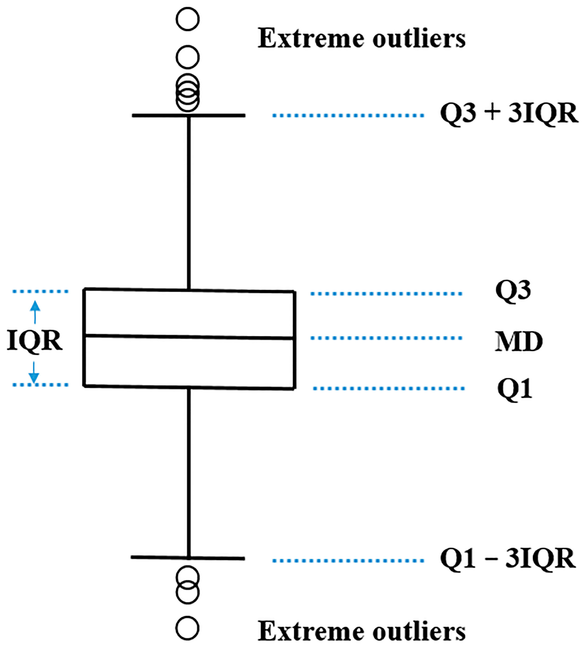
3.2. Outlier Detection

Outliers refer to extreme large and small values in each variable that are far away from the average level. Modeling directly with raw data may lead to model errors and result in distortion. Therefore, outliers were removed to ensure the reliability of machine learning model. A boxplot has proven to be a very effective tool for outlier detection [16,17,18]. The structure of a boxplot is shown in Figure 3. It mainly consists of five parts: upper quartile (Q3), median (MD), lower quartile (Q1), Q1 − 3IQR and Q3 + 3IQR. IQR represents the difference between Q3 and Q1. Those values between Q1 − 3IQR and Q3 + 3IQR are treated as effective data, while the others are treated as extreme outliers and deleted.

Figure 4 shows the outlier distribution of industrial data after it was normalized. It is seen that variables X₁–X₅ labeled as five kinds of chemical compositions in molten steel contain the most outliers, while the data of other variables are relatively stable. The reason can be summarized as follows: the detection of chemical composition was greatly affected by human factors, such as sampling and testing, while the other data collected by detection equipment in real time were rarely disturbed. Ultimately, the raw data were reduced to 2396 sets and the elimination ratio was 3.2%.

4. Feature Engineering

Feature engineering is another important task in the data preprocessing, and its main purpose is to select feature attributes that are strongly correlated with the target variable as the input items of the data-driven model. In the present section, Pearson correlation analysis was conducted to eliminate strong correlations among production parameters. After that, Grey relational analysis (GRA) was applied to pick out process parameters which strongly correlate with CSI.

4.1. Feature Correlation

Due to the complexity of continuous casting process of steel, there is inevitably a high correlation among variables. To some extent, information reflected by similar variables overlaps, which can lead to the problem of multicollinearity and increase the complexity of machine learning algorithms. Thus, Pearson correlation analysis was carried out to evaluate the correlations among variables, and the results were displayed visually by aid of a heatmap tool. Heatmap shows the correlations in terms of color gradients within the square. The lighter the color, the closer the absolute value of the correlation coefficient is to 1, which indicates a better correlation. The heatmap presentation of the correlations among continuous casting production parameters is shown in Figure 5. Generally, correlation coefficient greater than 0.6 indicates a strong correlation and one of them should be eliminated. Based on the above principle, secondary cooling water flow rate in zone 2 (X₇) and pouring temperature (X₁₀) was removed, and the secondary cooling intensity (X₉) and the superheat (X₁₂) were retained correspondingly.

4.2. Feature Selection

Feature selection is an important means to optimize the input items of data-driven models. The existence of redundant or irrelevant variables can not only lead to an increase of the data volume and computing burdens, but also make the network structure of machine learning algorithm more complex and deteriorate its generalization ability [19,20]. Hence, the purpose of feature selection is to remove weakly correlated variables and achieve dimension reduction.

In this study, GRA was used to screen out variables which had a strong correlation with the target variable CSI. GRA is an evaluation model that measures the degree of similarity between target variable sequence and feature variable sequence [21]. The level of correlation is evaluated by grey relational grade r_m (0 < r_m < 1). The larger the grey relational grade, the stronger the degree of closeness between the two sequences. The global comparison between two data sequences was undertaken instead of local comparison, so there is no side effect caused by subjective setting [22]. Besides, GRA is applicable to the amounts and regularity of the dataset and has the characteristic of simple calculation [23]. The steps of GRA are as follows [21,22,23]:

Step 1: select reference sequence P_{0 =} (P₀₁, P₀₂,⋯, P_0k) and compare sequence P_{i =} (P_i1, P_i2,⋯, P_ik), among them i = k = 1, 2,⋯, n.

Step 2: P₀ and P_i are normalized by the mean method. The formula is as follows:

$${P_i}^{\prime }=P_i(k)/\overline{P_i} , \overline{P_i}=\frac{1}{n}{\displaystyle \sum _{k=1}^1{P}_i}(k).$$

(3)

Step 3: Calculate the difference sequence, namely:

$${\Delta }_{oi}(k)=\left|P_0^{\prime }(k)-P_k^{\prime }(k)\right|.$$

(4)

The maximum and minimum values can be obtained from the above difference sequence, marked as $\underset{i}{\max } \underset{k}{\max }\left|P_0^{\prime }(k)-P_i^{\prime }(k)\right|$ and $\underset{i}{\min } \underset{k}{\min }\left|P_0^{\prime }(k)-P_i^{\prime }(k)\right|$.

Step 4: Correlation coefficient and grey relational grade are solved by Equation (5) and Equation (6), respectively:

$${\epsilon }_{0i}(k)=\frac{\underset{i}{\min } \underset{k}{\min }\left|P_0^{\prime }(k)-P_i^{\prime }(k)\right|+\rho \underset{i}{\max } \underset{k}{\max }\left|P_0^{\prime }(k)-P_i^{\prime }(k)\right|}{{\Delta }_{0i}(k)+\rho \underset{i}{\max } \underset{k}{\max }\left|P_0^{\prime }(k)-P_i^{\prime }(k)\right|},$$

(5)

$$r_m=\frac{1}{n}{\displaystyle \sum _{j=1}^n{\epsilon }_{oi}}(k),$$

(6)

where ρ (0 ≤ ρ ≤ 1) is known as the distinguishing coefficient, and ρ = 0.5 is used here.

Ultimately, the correlation sorting of all variables was achieved by GRA: X₁₁ > X₉ > X₁₄ > X₁₂ > X₈ > X₆ > X₁₃ > X₃ > X₂ > X₁ > X₄ > X₅. Although variables X₁–X₅ (five kinds of chemical compositions of molten steel) are correlated with CSI to some extent, they are low-ranking and should be eliminated.

5. Establishment of CSI Prediction Models

In this section, three models were established for CSI prediction based on MLR, ELM, and R-ELM algorithms, respectively. The implementation of the R-ELM model is described in detail, and the other two models are built as comparison models.

5.1. Multiple Linear Regression Model

MLR is a multivariate statistical technology, which has been widely used for online predictions due to its simple model structure and fast calculation speed. Therefore, the MLR model was introduced for CSI prediction based on the historical production data, and it was implemented using the Statistical Product and Service Solutions (SPSS®-version 25.0, IBM, Armonk, NY, USA) software. Since MLR requires all data to have original meaning, we used the raw data for modeling and validation. Among the historical production data, 2000 heats were used to establish the model and the other 476 heats were used to test the model. The regression equation is shown as follows:

CSI = −0.215 + 0.398X₁ + 0.049X₂ − 0.058X₃ + 0.013X₄ + 0.225X₅ + 0.013 × 10⁻⁵ X₆ −
     4.400 × 10⁻⁵ X₇ − 1.550 × 10⁻⁴X₈ − 1.380 × 10⁻⁴ X₉ + 7.000 × 10⁻⁶ X₁₀ − 0.028 X₁₁ +
2.000 × 10⁻³ X₁₂ + 5.380 × 10⁻⁴ X₁₃ + 8.647 × 10⁻³.

(7)

5.2. Extreme Learning Machine Model

ELM was first proposed by Huang et al. [24] in 2004, and it works on a simple structure named single-hidden layer feedforward neural networks [25]. The network structure of ELM is shown in Figure 6. ELM has a three-layer structure: input layer, hidden layer, and output layer. The input weights w_in in ELM are generated randomly without iterative solution, and only the output weight is calculated by the least square method. Thus, the learning speed of ELM can be much faster than that of traditional feedforward network algorithms, as well as better generalization performance. This algorithm can overcome the inherent defect of machine learning based on gradient descent learning theory, such as the local minima, the overtraining, and the high computing burdens [23,26]. Hence, it is suitable for online modeling with industrial data that are strongly coupled and nonlinear.

To establish the ELM model for CSI prediction, the processed industrial data were divided into two groups, of which 2000 heats were used to establish the model and the other 396 heats were used to test the model. The whole process was conducted using Matrix Laboratory (MATLAB®-version R2014a, MathWorks, Natick, MA, USA) software. After adjustments and tests, the highest prediction accuracy was obtained when the 7-20-1 three-layer structure was employed.

5.3. Regularized Extreme Learning Machine Model

As stated earlier, although ELM has the advantages of fewer setting parameters, faster learning speed, and stronger generalization ability compared with other artificial neural networks (ANNs), two major issues still remain in ELM [26,27,28,29]:

(1)

ELM is only based on the principle of empirical risk minimization and takes the training error minimization as the purpose, while does not take the structural risk into account. Hence, the problem of over-fitting still exists.

(2)

The computational robustness problems may occur when the hidden layer output matrix is a non-full column rank matrix or an ill-conditioned matrix because of its randomly generated input weights and biases.

It is evident that a model with good generalization ability should have a rational tradeoff between the empirical risk and structural risk. In order to overcome the above disadvantages of ELM, a regularized ELM was proposed by introducing structural risk into ELM. The implementation process of R-ELM is as follows [27].

The objective functions of R-ELM are expressed as Equations (8) and (9):

$$minE=min\frac{1}{2}{‖\beta ‖}^2+\frac{1}{2}\gamma {‖D\epsilon ‖}^2,$$

(8)

where ${‖\beta ‖}^2$ and ${‖D\epsilon ‖}^2$ are the structural risk and the empirical risk, respectively; γ is a weight factor used for adjusting the proportion of empirical risk and structural risk.

$${\epsilon }_j={\widehat{y}}_j-y_j=s.t.{\displaystyle {\sum }_{i=1}^N{\beta }_i}g({\omega }_i{x}_j+b_i)-t_j\hspace{1em}\hspace{1em}\left(j=1, 2, \dots , N\right) ,$$

(9)

where ε_j is the training error; x_j is the input; ${\widehat{y}}_j$ and $y_j$ are the predictive output and actual output, respectively; g is activation function of hidden layer neurons; ω_i and β_i are the input weight and output weight of the i th hidden layer node, respectively, and b_i is the threshold of hidden layer.

The Lagrange equation is built as follows:

$$L\left(\beta ,\epsilon ,\alpha \right)=\frac{1}{2}{‖\beta ‖}^2+\frac{\gamma }{2}{‖D\epsilon ‖}^2-\alpha \left(H\beta -T-\epsilon \right),$$

(10)

Take partial derivative for the above formula and the output weight matrix is obtained as follows:

$$\beta ={\left(\frac{I}{\gamma }+H^{T}H\right)}^{-1}{H}^{T}T,$$

(11)

where I is the identity matrix. The network output of R-ELM is as follows:

$$\widehat{y}={\sum }_{i=1}^L{\beta }_i{g}_i(x)={\sum }_{i=1}^L{\beta }_{i}g({\omega }_i·x+b_i).$$

(12)

After a series of formula derivation, the R-ELM algorithm was achieved with good generalization ability. In order to test its performance, the R-ELM model was established for CSI prediction using the same dataset as the ELM model. After continual adjustment and testing, the highest prediction accuracy can be achieved when the activation function is ‘Sigmoid’, γ is equal to 10-1, and 7-50-1 three-layer structure is employed.

6. Results and Discussion

The test results of the MLR model are shown in Figure 7 and Figure 8. As illustrated in Figure 7, the testing accuracy of the MLR model is evaluated by the correlation coefficient (R) between the predicted values and target values. The closer the correlation coefficient is to 1, the better the model performance will be. It is seen that there is a considerable discrepancy between predicted values and target values, and the correlation coefficient is only 0.577. Figure 8 shows the predictive error distribution of the MLR model. The predictive errors are mainly distributed within ±0.08%, and the prediction accuracy of the MLR model is 62% and 70%, respectively, when predictive errors are within ±0.025 and ±0.03. It is well known that MLR has an outstanding performance in dealing with linear regression problems. In this study, it simplifies the complex nonlinear problem into a linear one and ignores the interaction among variables, which eventually leads to a high ratio of misjudgment. Thus, this model can hardly provide a valuable guidance for online prediction of central carbon segregation of steel billets.

By contrast, the ELM model shows better performance than the MLR model. Figure 9 presents the linear regression of the target values and the predicted values of the ELM model. The results show that the predicted values agree well with the target values, and the correlation coefficient R is 0.813. Figure 10 indicates that the predictive errors of ELM model mainly distribute within a smaller range of ±0.07 compared with that of the MLR model. Moreover, when predictive errors are within ±0.025 and ±0.03, the prediction accuracy of ELM model reaches 84% and 90%, respectively. In particular, the computation time is only 0.02 s.

As expected, the test results of R-ELM model are the best among the three prediction models, which are shown in Figure 11 and Figure 12. It is obvious that the R-ELM model has the highest correlation coefficient (R = 0.871) and the most reasonable error distribution. When predictive errors are within ±0.025 and ±0.03, the prediction accuracy of R-ELM model is 89% and 94%, respectively. The high prediction accuracy of the R-ELM model is firstly attributed to the comprehensive data preprocessing efforts. Meanwhile, the introduction of tradeoff theory in the R-ELM algorithm also contributes to the high prediction accuracy. In summary, the R-ELM model could provide the most accurate predictions for CSI, and it shows potential for online quality evaluation of continuous casting steel billets.

In order to verify the correctness and generalization ability of the R-ELM model, the relationship between the key parameters and CSI was revealed based on the predictions of R-ELM model via response surface analysis. Besides, the reliability of the obtained conclusions was analyzed by means of metallurgical mechanism. Figure 13 shows the dependency of each parameter on CSI. As illustrated in Figure 13a, high superheat is a main factor leading to the increase of CSI [4,30,31], especially when the superheat is greater than 35 °C, and it is noted to rise dramatically. Lower superheat usually leads to a higher proportion of equiaxed structure, while higher superheat can promote the formation of ‘mini-ingots’. Therefore, keeping lower superheat is essential to suppress the central carbon segregation in continuous casting billets. CSI also increases along with the casting speed. Higher casting speed increases the solidification time of steel, and the secondary dendrite arm spacing increases correspondingly, which results in the enrichment of solute elements and aggravates the carbon segregation in steel billets.

As shown in Figure 13b, CSI decreases first and then increases with the increase of secondary cooling intensity. Generally, intense secondary cooling refines the dendritic structure and reduces the extent of segregation due to the reduced permeability of the mushy zone [5], however, it can also reduce the equiaxed crystal zoon and then aggravates segregation. Hence, a proper secondary cooling intensity is beneficial to improve the central carbon segregation in steel billets. The influence of water flow rate in zone1 on CSI is basically consistent with that of cooling intensity.

The results of response surface analysis are in accordance with the metallurgical mechanism, which verifies the correctness and generalization ability of the R-ELM model. Besides, the conclusions extracted from the predictions of the R-ELM model (also known as the “black-box” model) provide a definite control strategy for high carbon steel production. More importantly, this model is also applicable to other steel plants due to its high generalization ability.

To further verify the correctness and applicability of the R-ELM model, the central carbon segregation analysis of C80D steel samples was carried out by drilling method, and the obtained results were compared with the predicted values of the R-ELM model. The samples were collected from two casters with the same specifications. To ensure the accuracy of the experimental results, the CSI value was taken as the average value of three testing results. Figure 14 shows the comparison between experimental values and predicted values. As shown in Figure 14, experimental values agree well with predicted values, and the maximum error is only 0.023. The R-ELM model is expected to predict the CSI of steel billets in advance during the continuous casting process, which provides a supplementary means to guide timely the casting operation especially when the predicted value exceeds the required upper limit.

It should be noted that this work is only a tentative attempt to use machine learning algorithm to predict CSI and guide continuous casting production. Although the obtained results can be meaningful, the model remains to be further optimized. It is believed that with the further understanding of metallurgical phenomena and the development of intelligent algorithms, artificial intelligence has potential to find applications in continuous casting in the future.

7. Conclusions

In view of the complexity of continuous casting process of steel and the difficulty in predicting CSI accurately, this paper presents an improved R-ELM model for CSI prediction based on data preprocessing technologies. The main conclusions can be summarized as follows.

(1)

Boxplots can give a visual display of abnormal values in industrial data. GRA simplifies the neural network structure and further improves the hit ratio of data-driven models.

(2)

The test results indicate that the predicted values of the MLR model cannot agree well with target values. By contrast, the prediction accuracy of the ELM model is much higher. When predictive errors are within ±0.025 and ±0.03, the prediction accuracy is 84% and 90%, respectively. Moreover, the computation time is only 0.02 s.

(3)

In order to further improve the prediction accuracy and generalization ability of the ELM model, this paper proposed an R-ELM model for CSI prediction. The test results show that the prediction accuracy of R-ELM model is higher than that of the MLR model and the ELM model. When predictive errors are within ±0.03 and ±0.025, the prediction accuracy of R-ELM model is 94% and 89%, respectively. Additionally, the correlation coefficient between the target values and predicted values of the R-ELM model is 0.871, while the MLR model and ELM model are 0.571 and 0.813, respectively.

(4)

Response surface analysis was conducted on the predictions of the R-ELM model, and the results are consistent with metallurgical mechanism. Moreover, the test results of C80D steel samples from two casters agree well with the predicted values of the R-ELM model. The above conclusions further verify the correctness and generalization ability of the R-ELM model.

References

1. Zhao, R.J.; Fu, J.X.; Wu, Y.X.; Yang, Y.J.; Zhu, Y.Y.; Zhang, M. Representative technologies for hot charging and direct rolling in global steel industry. ISIJ Int. 2015, 55, 1816–1821. [Google Scholar]
2. Zhou, T.; Zhang, P.; Kuuskman, K.; Cerilli, E.; Cho, S.H.; Burella, D.; Zurob, H.S. Development of medium-to-high carbon hot-rolled steel strip on a thin slab casting direct strip production complex. Ironmak. Steelmak. 2017, 45, 603–610. [Google Scholar]
3. Pickering, E.J. Macrosegregation in steel ingots: The applicability of modelling and characterisation techniques. ISIJ Int. 2013, 53, 935–949. [Google Scholar] [CrossRef] [Green Version]
4. Ludlow, V.; Normanton, A.; Anderson, A.; Thiele, M.; Ciriza, J.; Laraudogoitia, J.; Knoop, W. Strategy to minimise central segregation in high carbon steel grades during billet casting. Ironmak. Steelmak. 2005, 32, 68–74. [Google Scholar] [CrossRef]
5. Choudhary, S.K.; Ganguly, S. Morphology and segregation in continuously cast high carbon steel billets. ISIJ Int. 2007, 47, 1759–1766. [Google Scholar] [CrossRef] [Green Version]
6. Vušanović, I.; Vertnik, R.; Šarler, B. A simple slice model for prediction of macrosegregation in continuously cast billets. In Proceedings of the 3rd International Conference on Advances in Solidification Processes, Aachen, The Netherlands, 7–10 June 2011. [Google Scholar]
7. Dong, Q.; Zhang, J.; Qian, L.; Yin, Y. Numerical modeling of macrosegregation in round billet with different microsegregation models. ISIJ Int. 2017, 57, 814–823. [Google Scholar] [CrossRef] [Green Version]
8. Combea, H.; Založnik, M.; Hans, S.; Richy, P.E. Prediction of macrosegregation in steel ingots: Influence of the motion and the morphology of equiaxed grains. Metall. Mat. Trans. B. 2009, 40, 289–304. [Google Scholar] [CrossRef]
9. Singh, A.K.; Basu, B.; Ghosh, A. Role of appropriate permeability model on numerical prediction of macrosegregation. Metall. Mat. Trans. B. 2006, 37, 799–809. [Google Scholar] [CrossRef]
10. García, P.J.; González, V.M.; Álvarez, J.C.; Bayón, R.M.; Sirgo, J.Á.; Díaz, A.M. A new predictive model of centerline segregation in continuous cast steel slabs by using multivariate adaptive regression splines approach. Materials 2015, 8, 3562–3583. [Google Scholar]
11. García, P.; García, E.; Álvarez, J.; González, V.; Mayo, R.; Mateos, F. A comparison of several machine learning techniques for the centerline segregation prediction in continuous cast steel slabs and evaluation of its performance. J. Comput. Appl. Math. 2018, 330, 877–895. [Google Scholar] [CrossRef]
12. Normanton, A.S.; Barber, B.; Bell, A.; Spaccarotella, A.; Holappa, L.; Laine, J.; Peters, H.; Link, N.; Ors, F.; Lopez, A.; et al. Developments in online surface and internal quality forecasting of continuously cast semis. Ironmak. Steelmak. 2004, 31, 376–382. [Google Scholar] [CrossRef]
13. Chen, H.Z.; Yang, J.P.; Lu, X.C.; Yu, X.Z.; Liu, Q. Quality prediction of the continuous casting bloom based on the extreme learning machine. Chin. J. Eng. 2018, 40, 815–821. [Google Scholar]
14. Davis, J.J.; Clark, A.J. Data preprocessing for anomaly based network intrusion detection: A review. Appl. Artif. Intell. 2011, 30, 353–375. [Google Scholar] [CrossRef]
15. Zhang, S.; Zhang, C.; Yang, Q. Data preparation for data mining. Appl. Artif. Intell. 2003, 17, 375–381. [Google Scholar] [CrossRef]
16. Cassar, D.R.; Carvalho, A.C.P.L.F.; Zanotto, E.D. Predicting glass transition temperatures using neural networks. Acta Mater. 2018, 159, 249–256. [Google Scholar] [CrossRef]
17. Aicha, A.B. Noninvasive detection of potentially precancerous lesions of vocal fold based on glottal wave signal and SVM approaches. Procedia Comput. Sci. 2018, 126, 586–595. [Google Scholar] [CrossRef]
18. Fan, C.; Xiao, F.; Yan, C. A framework for knowledge discovery in massive building automation data and its application in building diagnostics. Autom Constr. 2015, 50, 81–90. [Google Scholar] [CrossRef]
19. Pan, C.C.; Bai, J.; Yang, G.K.; Wong, D.S.H.; Jang, S.S. An inferential modeling method using enumerative PLS based nonnegative garrote regression. J. Process Control. 2012, 22, 1637–1646. [Google Scholar] [CrossRef]
20. He, F.; Zhang, L.Y. Prediction model of end-point phosphorus content in BOF steelmaking process based on PCA and BP neural network. J. Process Control 2018, 66, 51–58. [Google Scholar] [CrossRef]
21. Zhai, L.; Khoo, L.P.; Zhong, Z.W. Design concept evaluation in product development using rough sets and grey relation analysis. Expert Syst. Appl. 2009, 36, 7072–7079. [Google Scholar] [CrossRef]
22. Chan, J.W.K.; Tong, T.K.L. Multi-criteria material selections and end-of-life product strategy: Grey relational analysis approach. Mater. Des. 2007, 28, 1539–1546. [Google Scholar] [CrossRef]
23. Chen, W.; Kong, F.; Wang, B.; Li, Y. Application of grey relational analysis and extreme learning machine method for predicting silicon content of molten iron in blast furnace. Ironmak. Steelmak. 2018, 45, 1–6. [Google Scholar] [CrossRef]
24. Huang, G.B.; Zhu, Q.Y.; Siew, C.K. Extreme learning machine: Theory and applications. Neurocomputing 2006, 70, 489–501. [Google Scholar] [CrossRef]
25. Horata, P.; Chiewchanwattana, S.; Sunat, K. Robust extreme learning machine. Neurocomputing 2013, 102, 31–44. [Google Scholar] [CrossRef]
26. Wan, C.; Xu, Z.; Pinson, P.; Dong, Z.Y.; Wong, K.P. Probabilistic forecasting of wind power generation using extreme learning machine. IEEE Trans. Power Syst. 2014, 29, 1033–1044. [Google Scholar] [CrossRef] [Green Version]
27. Deng, W.; Zheng, Q.; Chen, L. Regularized extreme learning machine. In Proceedings of the 2009 IEEE Symposium on Computational Intelligence and Data Mining, Nashville, TN, USA, 30 March–2 April 2009; pp. 389–395. [Google Scholar]
28. Na, W.B.; Su, Z.W.; Ji, Y.F. Research of single well production prediction based on improved extreme learning machine. In Proceedings of the 2013 2nd International Conference on Measurement, Instrumentation and Automation, Guilin, China, 23–24 April 2013; pp. 1296–1300. [Google Scholar]
29. Huynh, H.T.; Won, Y. Regularized online sequential learning algorithm for single-hidden layer feedforward neural networks. Pattern Recogn. Lett. 2011, 32, 1930–1935. [Google Scholar] [CrossRef]
30. Scholes, A. Segregation in continuous casting. Ironmak. Steelmak. 2005, 32, 101–108. [Google Scholar] [CrossRef]
31. Huang, X.; Thomas, B.G.; Najjar, F.M. Modeling superheat removal during continuous casting of steel slabs. Metall. Mater. Trans. B. 1992, 23, 339–356. [Google Scholar] [CrossRef]
Figure 1. Workflow of central carbon segregation prediction.
Metals 09 01312 g001
Figure 2. Schematic diagrams of sampling (a) and drilling (b) in the steel billets.
Metals 09 01312 g002
Figure 3. The structure of a boxplot.
Metals 09 01312 g003
Figure 4. Boxplot presentation of outliers.
Metals 09 01312 g004
Figure 5. Variable correlations displayed by heatmap.
Metals 09 01312 g005
Figure 6. Network structure of the extreme learning machine (ELM).
Metals 09 01312 g006
Figure 7. Regression analysis between predicted and target values of CSI for the multiple linear regression (MLR) model.
Metals 09 01312 g007
Figure 8. Frequency distribution of predictive errors for the MLR model.
Metals 09 01312 g008
Figure 9. Regression analysis between predicted and target values of CSI for the ELM model.
Metals 09 01312 g009
Figure 10. Frequency distribution of predictive errors for the ELM model.
Metals 09 01312 g010
Figure 11. Regression analysis between predicted and target values of CSI for the regularized ELM (R-ELM) model.
Metals 09 01312 g011
Figure 12. Frequency distribution of predictive errors for the R-ELM model.
Metals 09 01312 g012
Figure 13. Response surfaces of the R-ELM prediction model for different combinations of input variables: (a) superheat and casting speed, (b) cooling intensity and water flow rate in zone1.
Metals 09 01312 g013
Figure 14. Experimental and predicted values of central carbon segregation in steel billets.
Metals 09 01312 g014