Density-Sensitive Implicit Functions Using Sub-Voxel Sampling in Additive Manufacturing

 , ,
, ,  and
and
Abstract
1. Introduction
2. Literature Review
2.1. Topology Optimization in Additive Manufacturing
2.2. Lattice Structures in Additive Manufacturing
2.3. Explicit Realization of the Results of Topology Optimization into Surface-Based Lattices
2.4. Conclusions of the Literature Review
3. Methodology
3.1. Formulation of SIMP
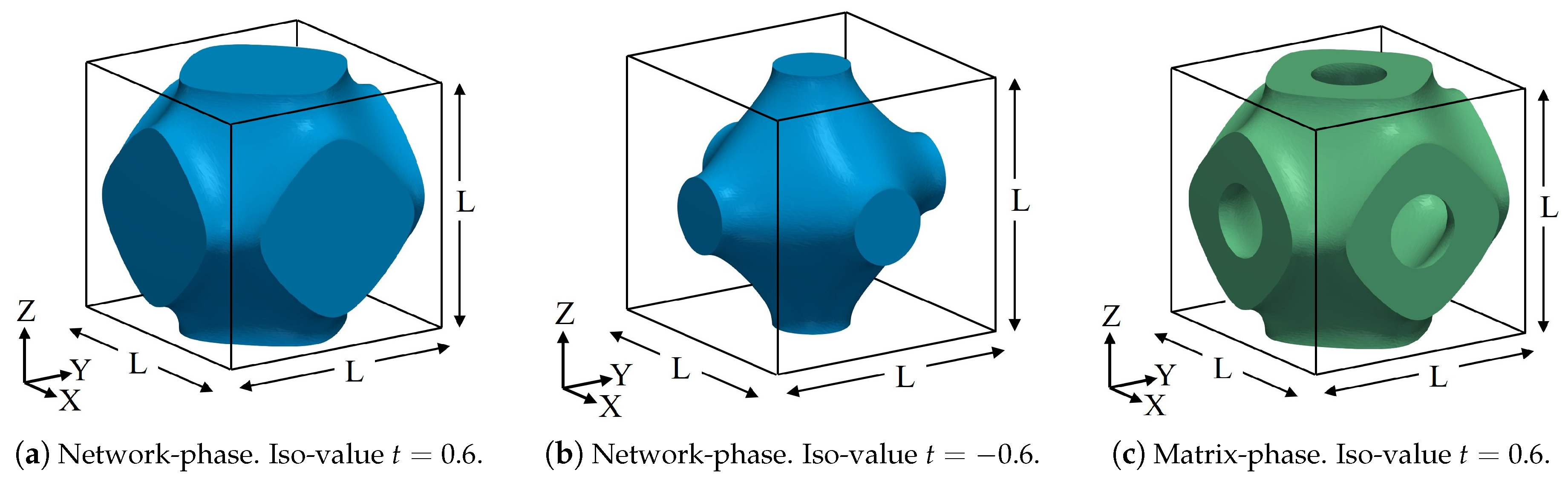
3.2. Morphology of Schwarz Primitive Lattice Structures
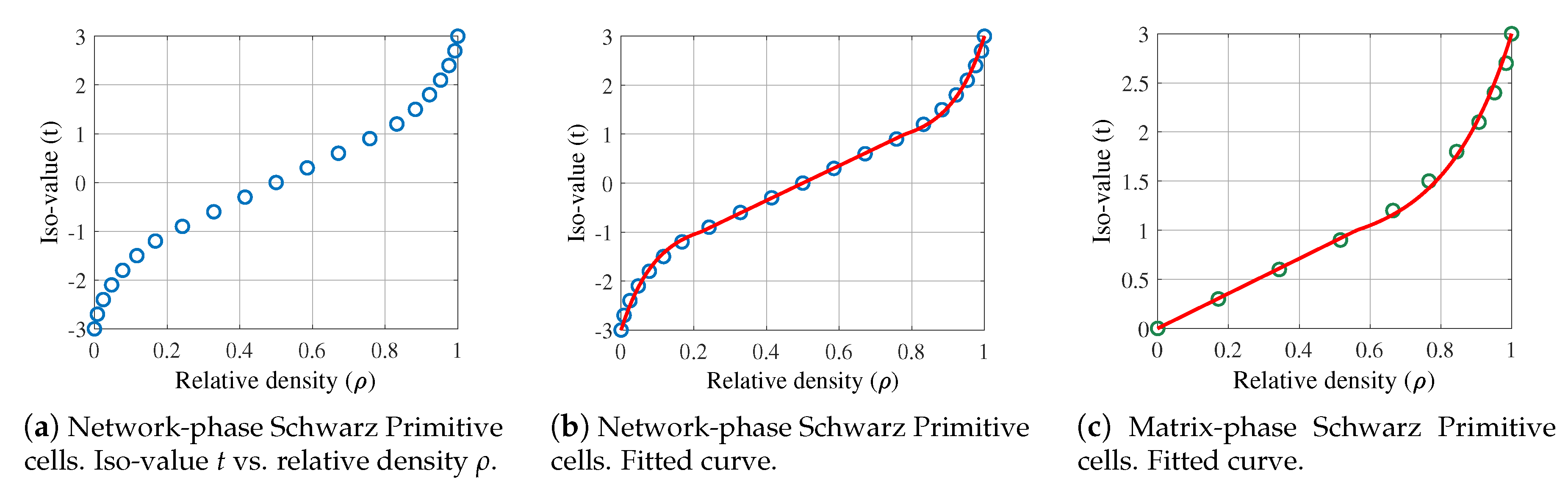
3.3. Relation between the Iso-Value and the Relative Density of Schwarz Primitive Cells
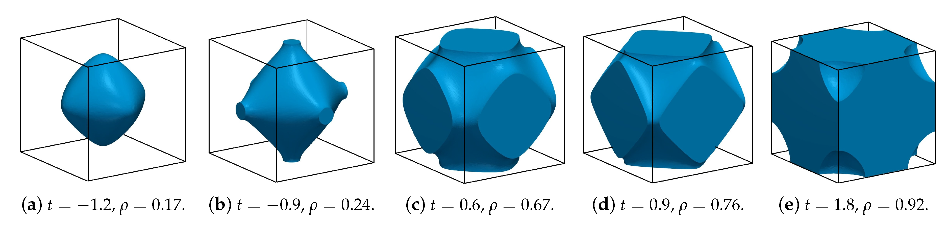
3.3.1. Network-Phase Cells
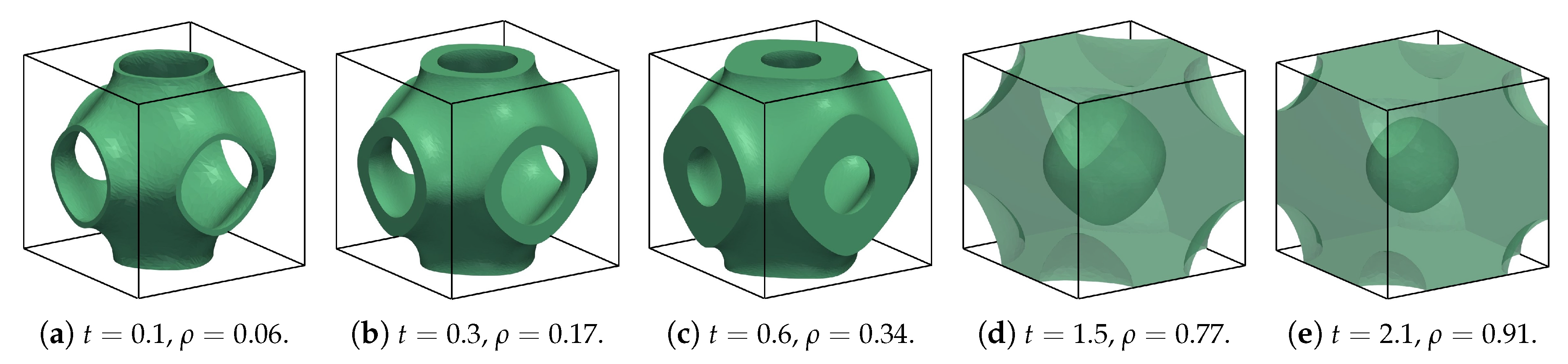
3.3.2. Matrix-Phase Cells
3.4. Derivation of the Lattice Iso-Value as Function of the Relative Density
3.4.1. Network-Phase Cells
3.4.2. Matrix-Phase Cells
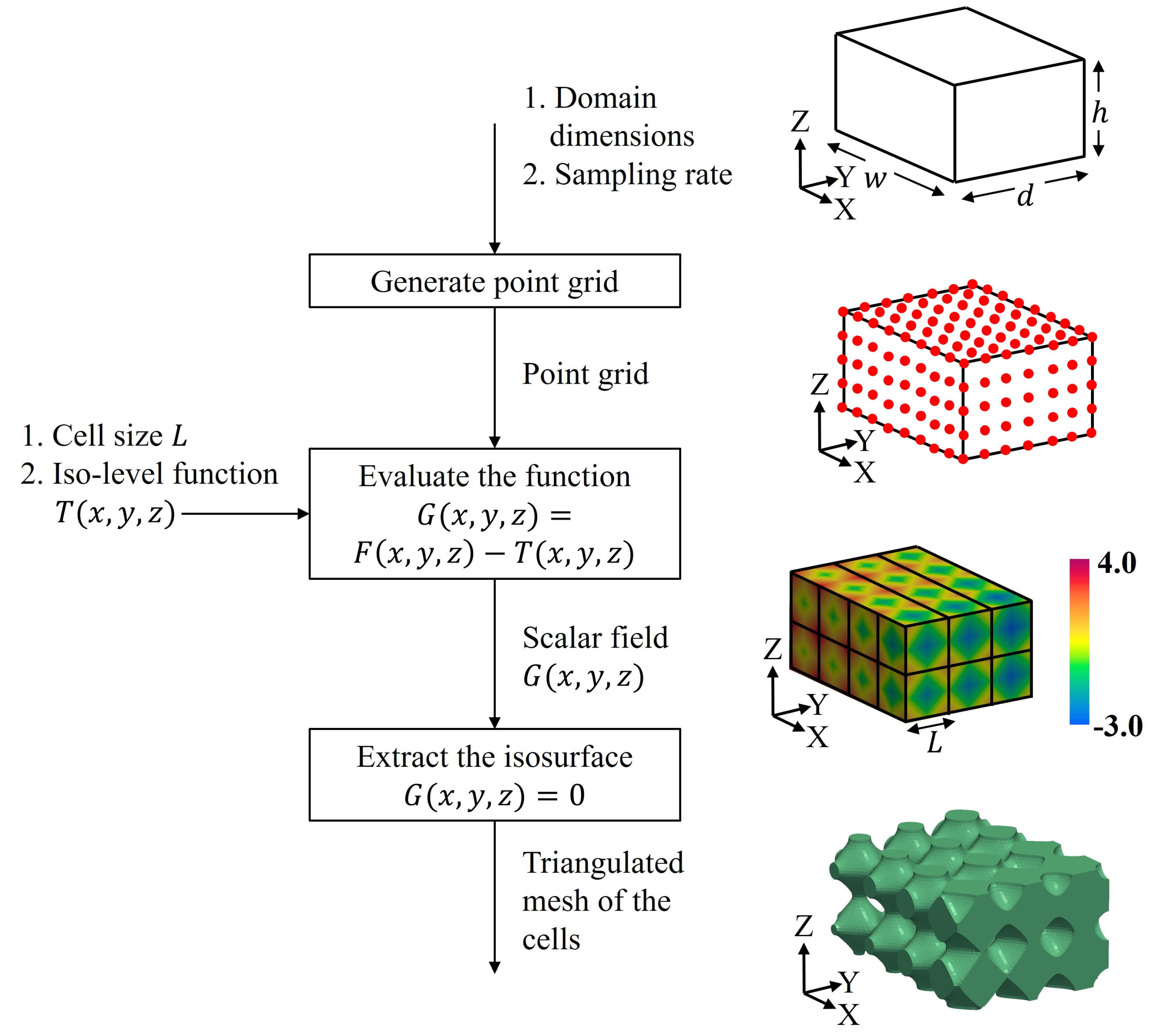
3.5. Generation of Variable-Density Surface Lattice Structures
- Generation of the point grid: the first step is to sample , given its dimensions and the grid sampling rate in which must be sampled. The output of this step is a point grid.
- Evaluation of the function : the function G is evaluated in the point grid obtained in the previous step. Apart from the point grid, it is necessary to provide (1) the size of the cell (L in Equation (4)), and (2) the iso-level function T. The outcome of this step is the scalar field .
- Extraction of the isosurface : the final step is to retrieve the isosurface from the scalar field generated in step 2 using Marching Cubes algorithm. This algorithm returns a triangular mesh that approximates the required isosurface.
3.6. Explicit Realization of a Density Field into Variable-Density Surface Lattice Structures: Problem Statement
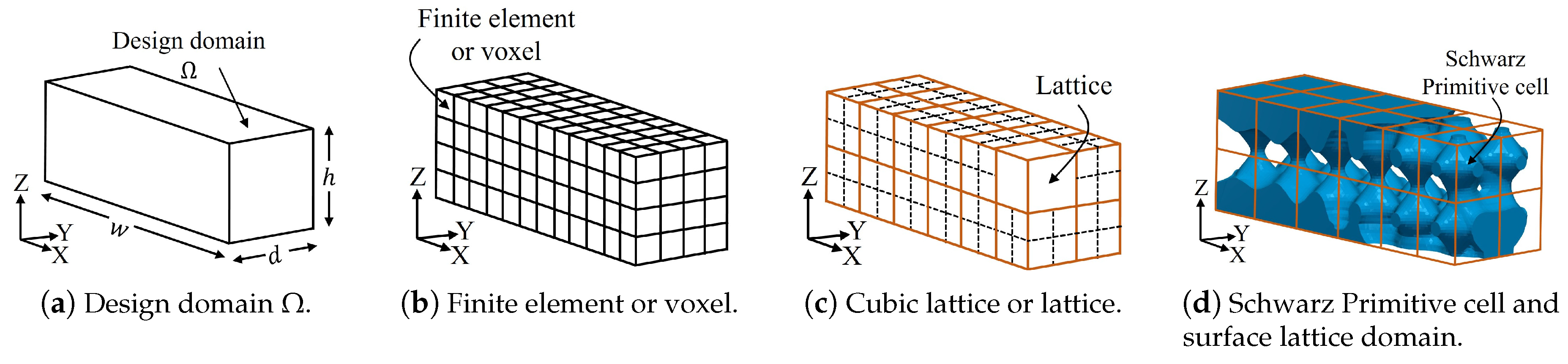
- A prismatic rectangular domain orthogonally oriented with respect to the World Coordinate System.
- A set E of cubic voxels, which partition , defined by a regular orthogonal grid. This set of voxels serve as FEA elements in the topology optimization.
- A density map defined on E, that is, , where represents the relative density of the i-th voxel (e.g., the dictated by the topology optimization algorithms).
- To generate a scalar (iso-value) function such that:
- (a)
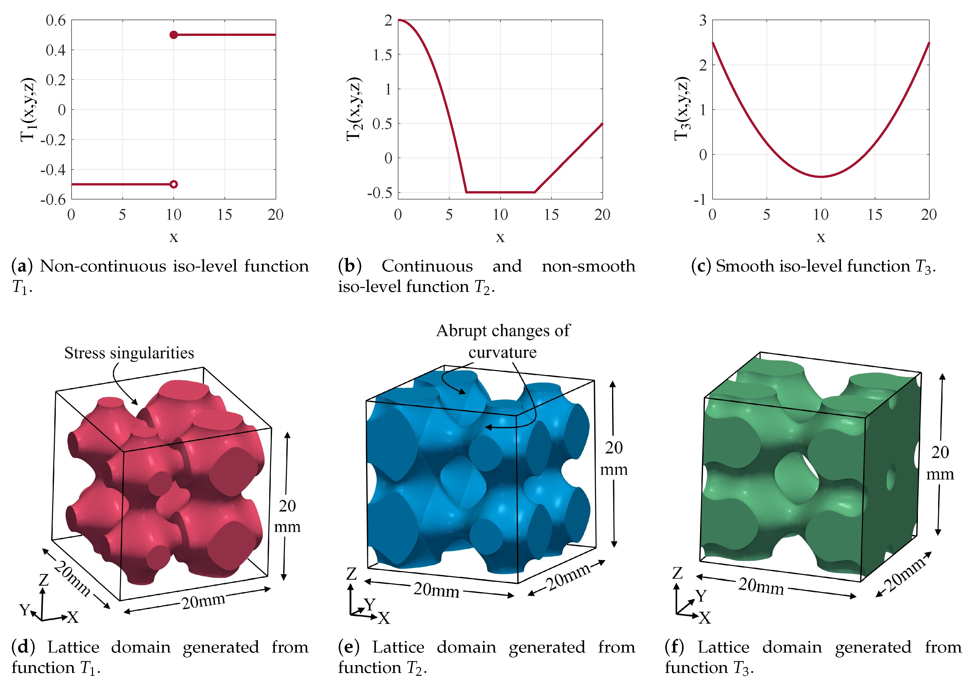
- T is bounded. In the Schwarz-modified case used in this work, , to ensure that the domain is not devoid of material.
- (b)
- T is continuous.
- (c)
- , where denotes the relative density of a periodic Schwarz cell with tuning parameter t. That is, for every point , the density induced at that point by the function T must be equal to the density of the voxel to which the point belongs.
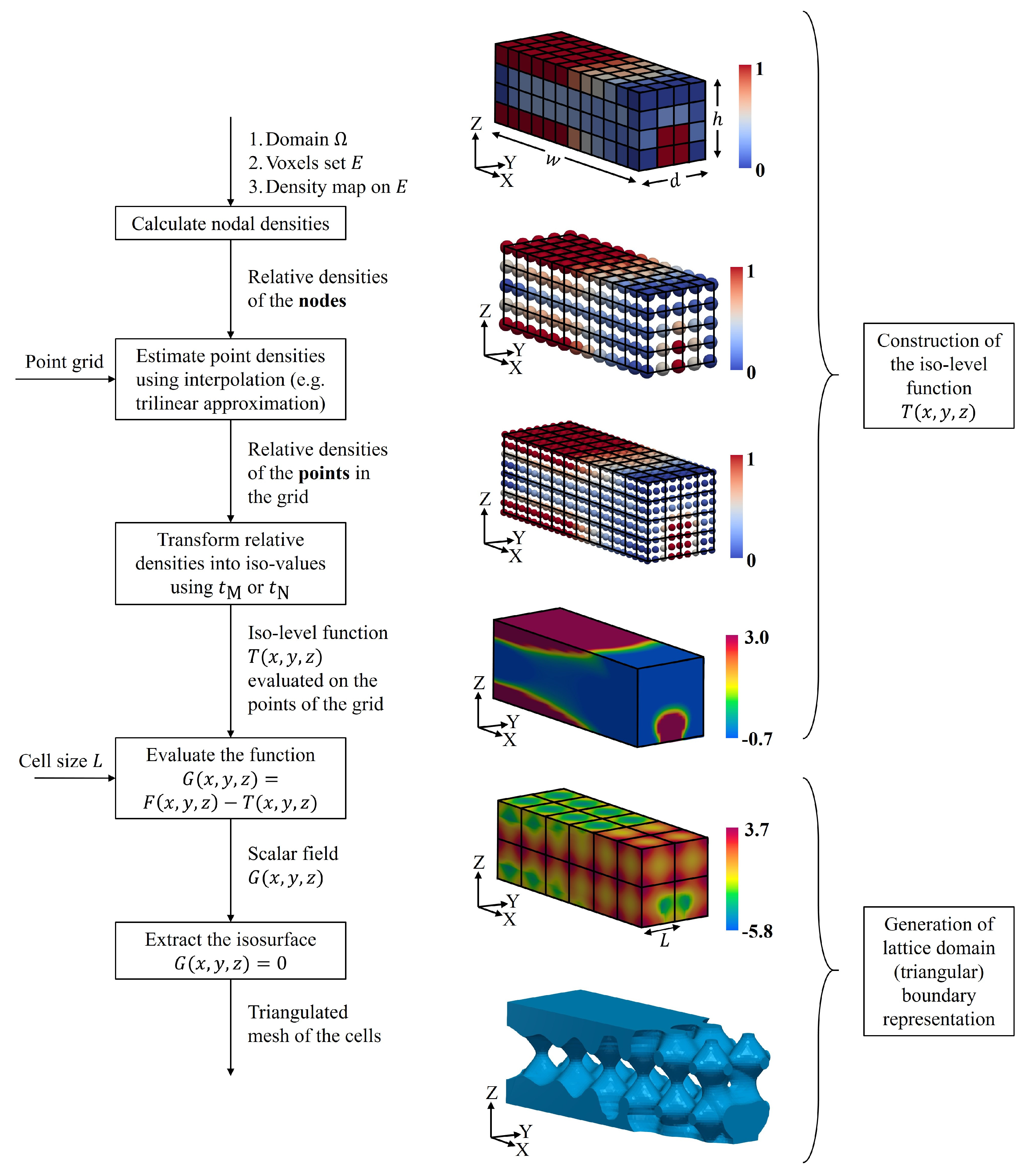
3.7. Explicit Realization of a Density Field into Variable-Density Surface Lattice Structures: Problem Solution
- Calculation of the vertex densities: in this step, the densities of the vertices Q of the voxels are computed. Let be a vertex that belongs to the voxels . The density of q is defined in Equation (16).
- Estimation of the densities of the points in the grid: once the vertex densities are calculated, these can be used to estimate the density of every point . Assuming (1) are the vertices of voxel , (2) are the vertex densities and (3) , the relative density of the point p is given by , (), where H is an interpolation function. This work uses trilinear interpolation for the simulations.
- Transformation of the relative densities into iso-values: the relative density of each point of the grid must be transformed into its corresponding iso-value. The function (or ) in Equation (7) (or Equation (9)) is used for this task. Therefore, the iso-level function of element is . If the number of voxels is N, the obtained iso-level function T is:It is important to remark that the function in Equation (17) is a piece-wise continuous function.
4. Results
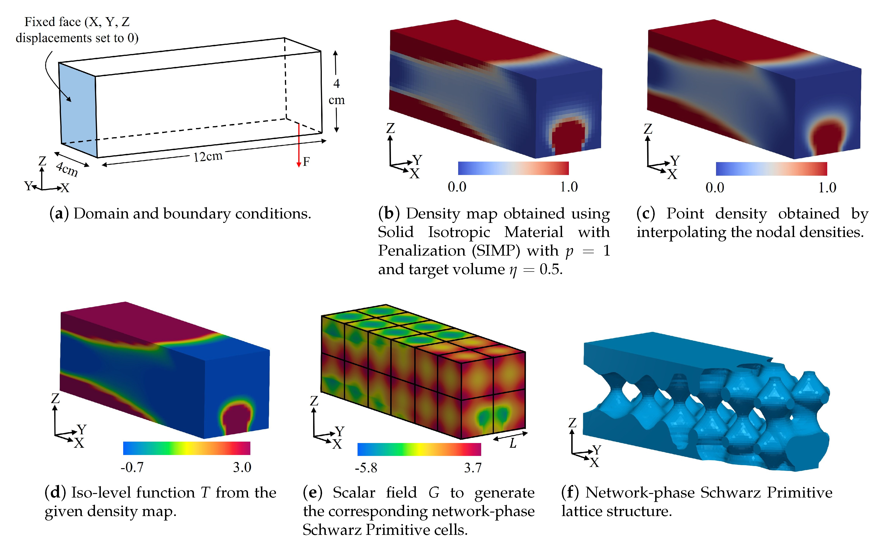
4.1. Density Field into Surface Lattice Structures. Applications in Topology Optimization
4.2. Physical Realization of the Devised Lattice Structures
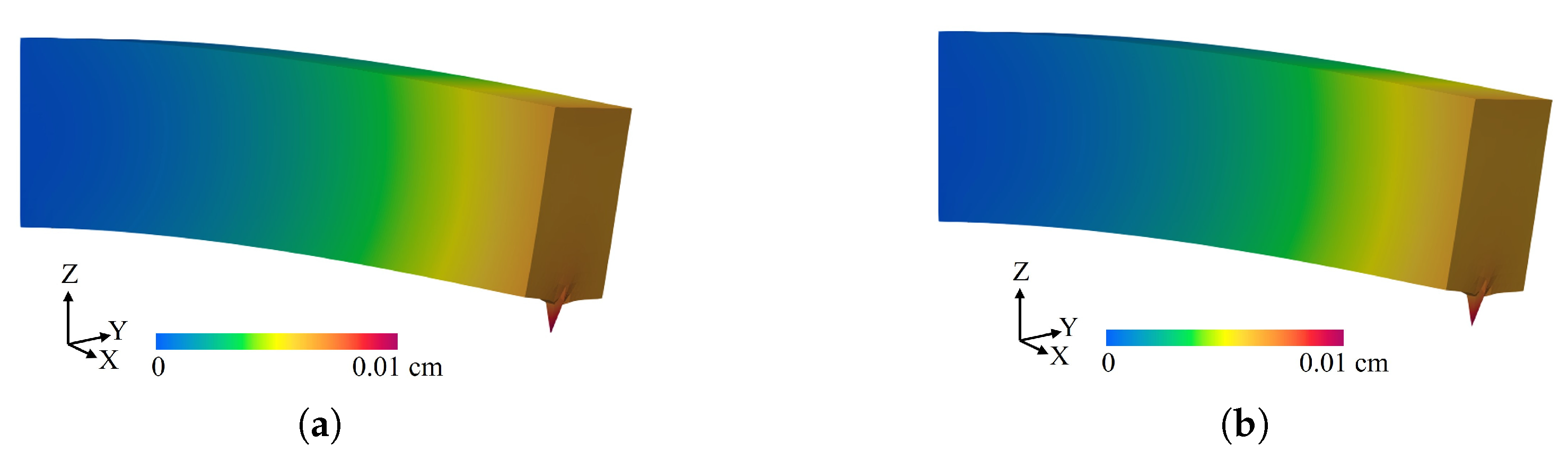
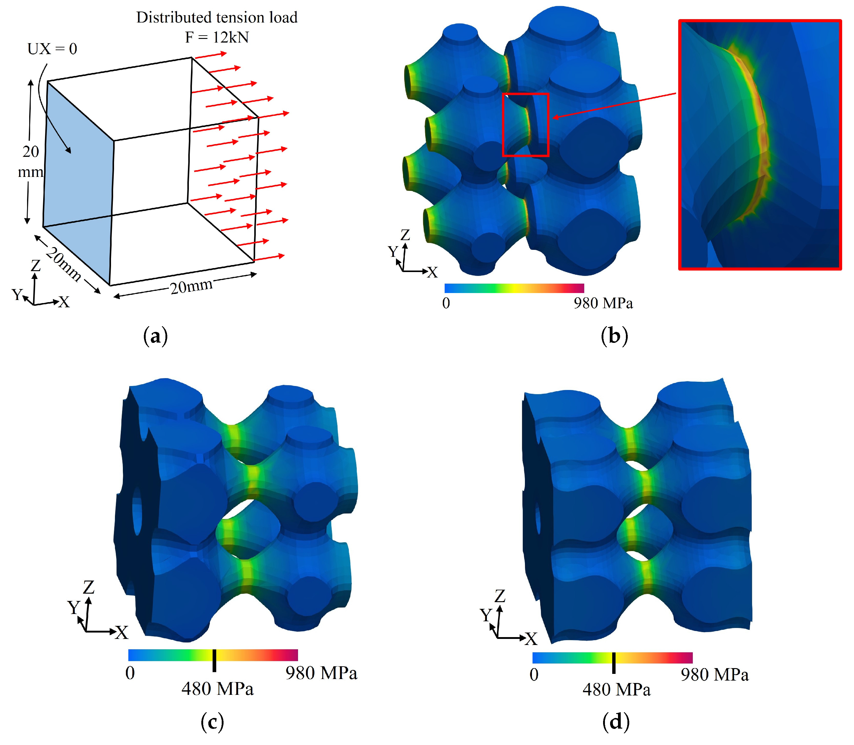
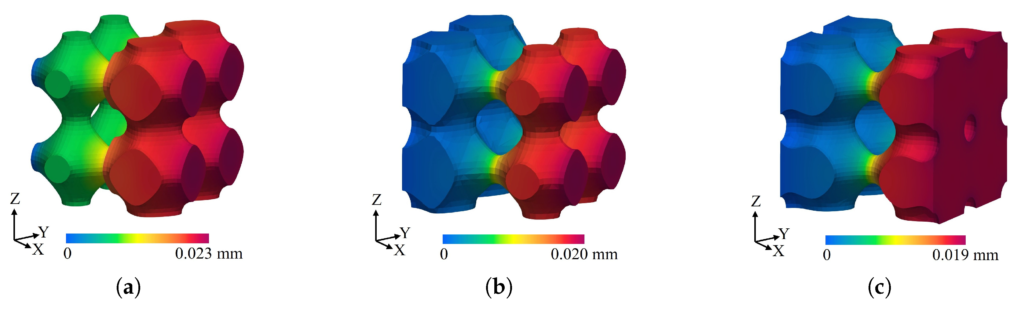
4.3. Stress Concentration in Variable-Density Surface Lattice Structures
5. Conclusions
Author Contributions
Funding
Conflicts of Interest
Abbreviations
| B-Rep: | Boundary representation of a solid object in . | |
| FEA: | Finite element analysis. | |
| SIMP: | Solid isotropic material with penalization, which is a topology optimization algorithm. | |
| : | , , denotes the compliance or total strain energy of a domain with vector of relative densities (J). | |
| : | Penalty factor aimed to polarize element relative densities around 0 and 1. | |
| : | Fraction of volume to be retained (or target volume) in the final design. | |
| V: | , , denotes the volume of a domain with vector of relative densities (mm or cm). | |
| : | Volume of the design domain (mm or cm). | |
| : | Young’s modulus of the bulk material (Pa). | |
| : | Young’s modulus of the i-th element of the mesh (Pa). | |
| L: | Length of the surface lattice cell (mm or cm). | |
| : | Relative density or volume fraction of a Schwarz Primitive. | |
| : | The function returns the relative density of a Schwarz Primitive cell generated with an iso-value t. | |
| (or ): | The function (or ) returns the relative density of a network-phase (or matrix-phase) Schwarz Primitive cell generated with an iso-value t. | |
| (or ): | The function (or ) gives the relative density of an element (or node ) of the mesh. | |
| : | Iso-value to generate a Schwarz Primitive cell. Tuning parameter related but not equal to the thickness of the walls of the cell. | |
| : | The function returns the iso-value that generates a Schwarz Primitive cell of relative density . | |
| (or ): | The function (or ) returns the iso-value that generates a network-phase (or matrix-phase) Schwarz Primitive cell of relative density . | |
| : | is the implicit function that characterizes the Schwarz Primitive surfaces. | |
| : | The iso-level function () used to produce variable-density surface lattice structures. The function T is the generalization of the value t. | |
| : | Scalar field that is evaluated to generate variable-density surface lattice structures. | |
| : | Rectangular prismatic subset of , which represents the design domain. | |
| : | Width, depth and height of (mm or cm). | |
| : | Partition of into voxels. The set denotes the voxels and the set denotes the vertices of the voxels. | |
| H: | Interpolation function. In this manuscript refers to tri-linear interpolation of point p given the values . | |
| : | Vector of relative densities of the N elements of the mesh M. | |
Appendix A. Iso-Level Functions

| Figure Numbers | Iso-Level Function |
|---|---|
| Figure 15a,d | |
| Figure 15b,e | |
| Figure 15c,f |
References
- Posada, J.; Toro, C.; Barandiaran, I.; Oyarzun, D.; Stricker, D.; de Amicis, R.; Pinto, E.B.; Eisert, P.; Döllner, J.; Vallarino, I. Visual Computing as a Key Enabling Technology for Industrie 4.0 and Industrial Internet. IEEE Comput. Graph. Appl. 2015, 35, 26–40. [Google Scholar] [CrossRef]
- Gao, W.; Zhang, Y.; Ramanujan, D.; Ramani, K.; Chen, Y.; Williams, C.B.; Wang, C.C.; Shin, Y.C.; Zhang, S.; Zavattieri, P.D. The status, challenges, and future of additive manufacturing in engineering. Comput.-Aided Des. 2015, 69, 65–89. [Google Scholar] [CrossRef]
- Liu, J.; Gaynor, A.T.; Chen, S.; Kang, Z.; Suresh, K.; Takezawa, A.; Li, L.; Kato, J.; Tang, J.; Wang, C.C.L.; et al. Current and future trends in topology optimization for additive manufacturing. Struct. Multidiscip. Optim. 2018, 57, 2457–2483. [Google Scholar] [CrossRef]
- Hou, W.; Yang, X.; Zhang, W.; Xia, Y. Design of energy-dissipating structure with functionally graded auxetic cellular material. Int. J. Crashworthin. 2018, 23, 366–376. [Google Scholar] [CrossRef]
- Maloney, K.J.; Fink, K.D.; Schaedler, T.A.; Kolodziejska, J.A.; Jacobsen, A.J.; Roper, C.S. Multifunctional heat exchangers derived from three-dimensional micro-lattice structures. Int. J. Heat Mass Transf. 2012, 55, 2486–2493. [Google Scholar] [CrossRef]
- Yin, S.; Wu, L.; Yang, J.; Ma, L.; Nutt, S. Damping and low-velocity impact behavior of filled composite pyramidal lattice structures. J. Compos. Mater. 2014, 48, 1789–1800. [Google Scholar] [CrossRef]
- Liu, J.; Ma, Y. A survey of manufacturing oriented topology optimization methods. Adv. Eng. Softw. 2016, 100, 161–175. [Google Scholar] [CrossRef]
- Montoya-Zapata, D.; Acosta, D.A.; Moreno, A.; Posada, J.; Ruiz-Salguero, O. Sensitivity Analysis in Shape Optimization using Voxel Density Penalization. In Spanish Computer Graphics Conference (CEIG); Casas, D., Jarabo, A., Eds.; The Eurographics Association: Geneve, Switzerland, 2019. [Google Scholar] [CrossRef]
- Sigmund, O. A 99 line topology optimization code written in Matlab. Struct. Multidiscip. Optim. 2001, 21, 120–127. [Google Scholar] [CrossRef]
- Montoya-Zapata, D.; Acosta, D.A.; Ruiz-Salguero, O.; Posada, J.; Sanchez-Londono, D. A General Meta-graph Strategy for Shape Evolution under Mechanical Stress. Cybern. Syst. 2019, 50, 3–24. [Google Scholar] [CrossRef]
- Tang, Y.; Kurtz, A.; Zhao, Y.F. Bidirectional Evolutionary Structural Optimization (BESO) based design method for lattice structure to be fabricated by additive manufacturing. Comput.-Aided Des. 2015, 69, 91–101. [Google Scholar] [CrossRef]
- Liu, J.; Yu, H.; To, A.C. Porous structure design through Blinn transformation–based level set method. Struct. Multidiscip. Optim. 2018, 57, 849–864. [Google Scholar] [CrossRef]
- Langelaar, M. Topology optimization of 3D self–supporting structures for additive manufacturing. Addit. Manuf. 2016, 12, 60–70. [Google Scholar] [CrossRef]
- Vanek, J.; Galicia, J.A.G.; Benes, B. Clever Support: Efficient Support Structure Generation for Digital Fabrication. Comput. Graph. Forum 2014, 33, 117–125. [Google Scholar] [CrossRef]
- Panesar, A.; Abdi, M.; Hickman, D.; Ashcroft, I. Strategies for functionally graded lattice structures derived using topology optimisation for Additive Manufacturing. Addit. Manuf. 2018, 19, 81–94. [Google Scholar] [CrossRef]
- Wu, J.; Wang, C.C.; Zhang, X.; Westermann, R. Self-supporting rhombic infill structures for additive manufacturing. Comput.-Aided Des. 2016, 80, 32–42. [Google Scholar] [CrossRef]
- Lee, D.W.; Khan, K.A.; Al-Rub, R.K.A. Stiffness and yield strength of architectured foams based on the Schwarz Primitive triply periodic minimal surface. Int. J. Plast. 2017, 95, 1–20. [Google Scholar] [CrossRef]
- Montoya-Zapata, D.; Cortés, C.; Ruiz-Salguero, O. FE-simulations with a simplified model for open-cell porous materials: A Kelvin cell approach. J. Comput. Methods Sci. Eng. 2019, 19, 989–1000. [Google Scholar] [CrossRef]
- Elmadih, W.; Syam, W.P.; Maskery, I.; Chronopoulos, D.; Leach, R. Mechanical vibration bandgaps in surface-based lattices. Addit. Manuf. 2019, 25, 421–429. [Google Scholar] [CrossRef]
- Helou, M.; Kara, S. Design, analysis and manufacturing of lattice structures: an overview. Int. J. Comput. Integr. Manuf. 2018, 31, 243–261. [Google Scholar] [CrossRef]
- Melchels, F.P.; Bertoldi, K.; Gabbrielli, R.; Velders, A.H.; Feijen, J.; Grijpma, D.W. Mathematically defined tissue engineering scaffold architectures prepared by stereolithography. Biomaterials 2010, 31, 6909–6916. [Google Scholar] [CrossRef]
- Ataee, A.; Li, Y.; Fraser, D.; Song, G.; Wen, C. Anisotropic Ti-6Al-4V gyroid scaffolds manufactured by electron beam melting (EBM) for bone implant applications. Mater. Des. 2018, 137, 345–354. [Google Scholar] [CrossRef]
- Li, D.; Liao, W.; Dai, N.; Dong, G.; Tang, Y.; Xie, Y.M. Optimal design and modeling of gyroid-based functionally graded cellular structures for additive manufacturing. Comput.-Aided Des. 2018, 104, 87–99. [Google Scholar] [CrossRef]
- Strano, G.; Hao, L.; Everson, R.M.; Evans, K.E. A new approach to the design and optimisation of support structures in additive manufacturing. Int. J. Adv. Manuf. Technol. 2013, 66, 1247–1254. [Google Scholar] [CrossRef]
- Afshar, M.; Anaraki, A.P.; Montazerian, H.; Kadkhodapour, J. Additive manufacturing and mechanical characterization of graded porosity scaffolds designed based on triply periodic minimal surface architectures. J. Mech. Behav. Biomed. Mater. 2016, 62, 481–494. [Google Scholar] [CrossRef] [PubMed]
- Yan, C.; Hao, L.; Hussein, A.; Raymont, D. Evaluations of cellular lattice structures manufactured using selective laser melting. Int. J. Mach. Tools Manuf. 2012, 62, 32–38. [Google Scholar] [CrossRef]
- Brackett, D.; Ashcroft, I.; Hague, R. Topology optimization for additive manufacturing. In Proceedings of the Solid Freeform Fabrication Symposium, Austin, TX, USA, 8–10 August 2011; Volume 1, pp. 348–362. [Google Scholar]
- Song, G.H.; Jing, S.K.; Zhao, F.L.; Wang, Y.D.; Xing, H.; Zhou, J.T. Design Optimization of Irregular Cellular Structure for Additive Manufacturing. Chin. J. Mech. Eng. 2017, 30, 1184–1192. [Google Scholar] [CrossRef]
- Zhang, P.; Toman, J.; Yu, Y.; Biyikli, E.; Kirca, M.; Chmielus, M.; To, A.C. Efficient Design–Optimization of Variable-Density Hexagonal Cellular Structure by Additive Manufacturing: Theory and Validation. J. Manuf. Sci. Eng. 2015, 137, 021004. [Google Scholar] [CrossRef]
- Alzahrani, M.; Choi, S.K.; Rosen, D.W. Design of truss-like cellular structures using relative density mapping method. Mater. Des. 2015, 85, 349–360. [Google Scholar] [CrossRef]
- Liu, X.; Shapiro, V. Sample–Based Design of Functionally Graded Material Structures. In Proceedings of the ASME 2016 International Design Engineering Technical Conferences and Computers and Information in Engineering Conference, Charlotte, NC, USA, 21–24 August 2016; p. 02. [Google Scholar] [CrossRef]
- Savio, G.; Meneghello, R.; Concheri, G. Design of variable thickness triply periodic surfaces for additive manufacturing. Prog. Addit. Manuf. 2019, 4, 281–290. [Google Scholar] [CrossRef]
- Liu, K.; Tovar, A. An efficient 3D topology optimization code written in Matlab. Struct. Multidiscip. Optim. 2014, 50, 1175–1196. [Google Scholar] [CrossRef]
- Wohlgemuth, M.; Yufa, N.; Hoffman, J.; Thomas, E.L. Triply Periodic Bicontinuous Cubic Microdomain Morphologies by Symmetries. Macromolecules 2001, 34, 6083–6089. [Google Scholar] [CrossRef]
- Maskery, I.; Sturm, L.; Aremu, A.; Panesar, A.; Williams, C.; Tuck, C.; Wildman, R.; Ashcroft, I.; Hague, R. Insights into the mechanical properties of several triply periodic minimal surface lattice structures made by polymer additive manufacturing. Polymer 2018, 152, 62–71. [Google Scholar] [CrossRef]
- Al-Ketan, O.; Al-Rub, R.K.A. Multifunctional Mechanical Metamaterials Based on Triply Periodic Minimal Surface Lattices. Adv. Eng. Mater. 2019, 21. [Google Scholar] [CrossRef]
- Ahrens, J.; Geveci, B.; Law, C. ParaView: An End-User Tool for Large-Data Visualization. In Visualization Handbook; Hansen, C.D., Johnson, C.R., Eds.; Butterworth-Heinemann: Burlington, MA, USA, 2005; pp. 717–731. [Google Scholar] [CrossRef]
- Liu, S.; Shin, Y.C. Additive manufacturing of Ti6Al4V alloy: A review. Mater. Des. 2019, 164, 107552. [Google Scholar] [CrossRef]


| Domain | Figure Number | Volume (cm) | Percentage of Material Saving (%) |
|---|---|---|---|
| Network-phase from original SIMP | Figure 10a | () | |
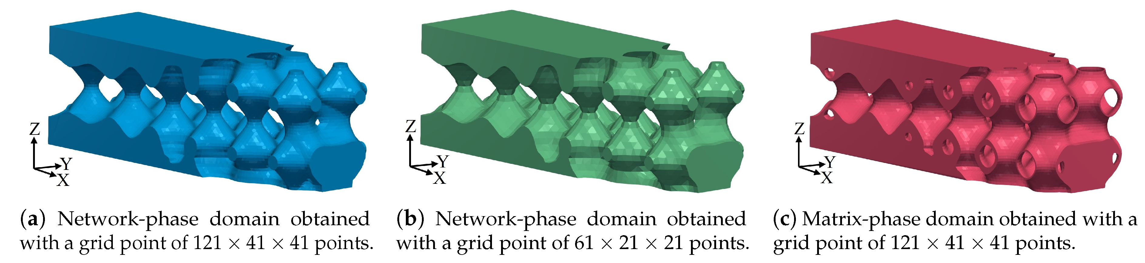
| Network-phase from original SIMP and point grid of | Figure 10b | () | |
| Matrix-phase from original SIMP | Figure 10c | () | |
| Network-phase from modified SIMP with | Figure 11b | () | |
| Matrix-phase from modified SIMP with | Figure 11c | () |
| Domain | Figures | Size | Machine | Technology | Bulk Material | Layer Thickness | Build Direction | Support Material | Heat Treatment |
|---|---|---|---|---|---|---|---|---|---|
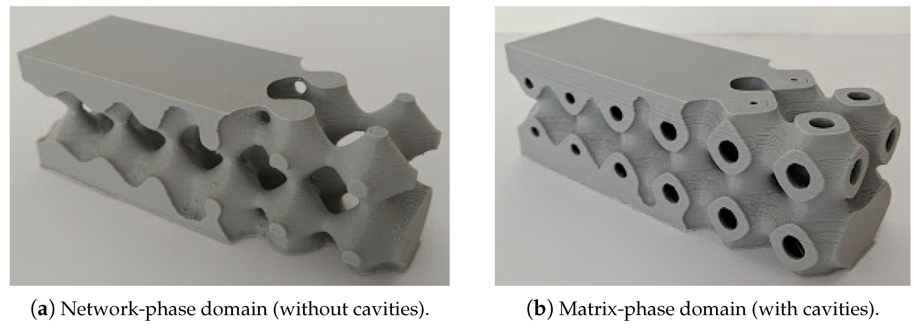
| Network-phase domain in Figure 11b (without cavities) | Figure 13a | 12 cm × 4 cm × 4 cm | Atom 2.0 | Fused Deposition Modeling | PLA (Polylactic acid) | 200 m | Z axis in Figure 11a | No | No |
| Matrix-phase domain in Figure 11c (with cavities) | Figure 13b | 12 cm × 4 cm × 4 cm | Atom 2.0 | Fused Deposition Modeling | PLA (Polylactic acid) | 200 m | Z axis in Figure 11a | Yes | No |
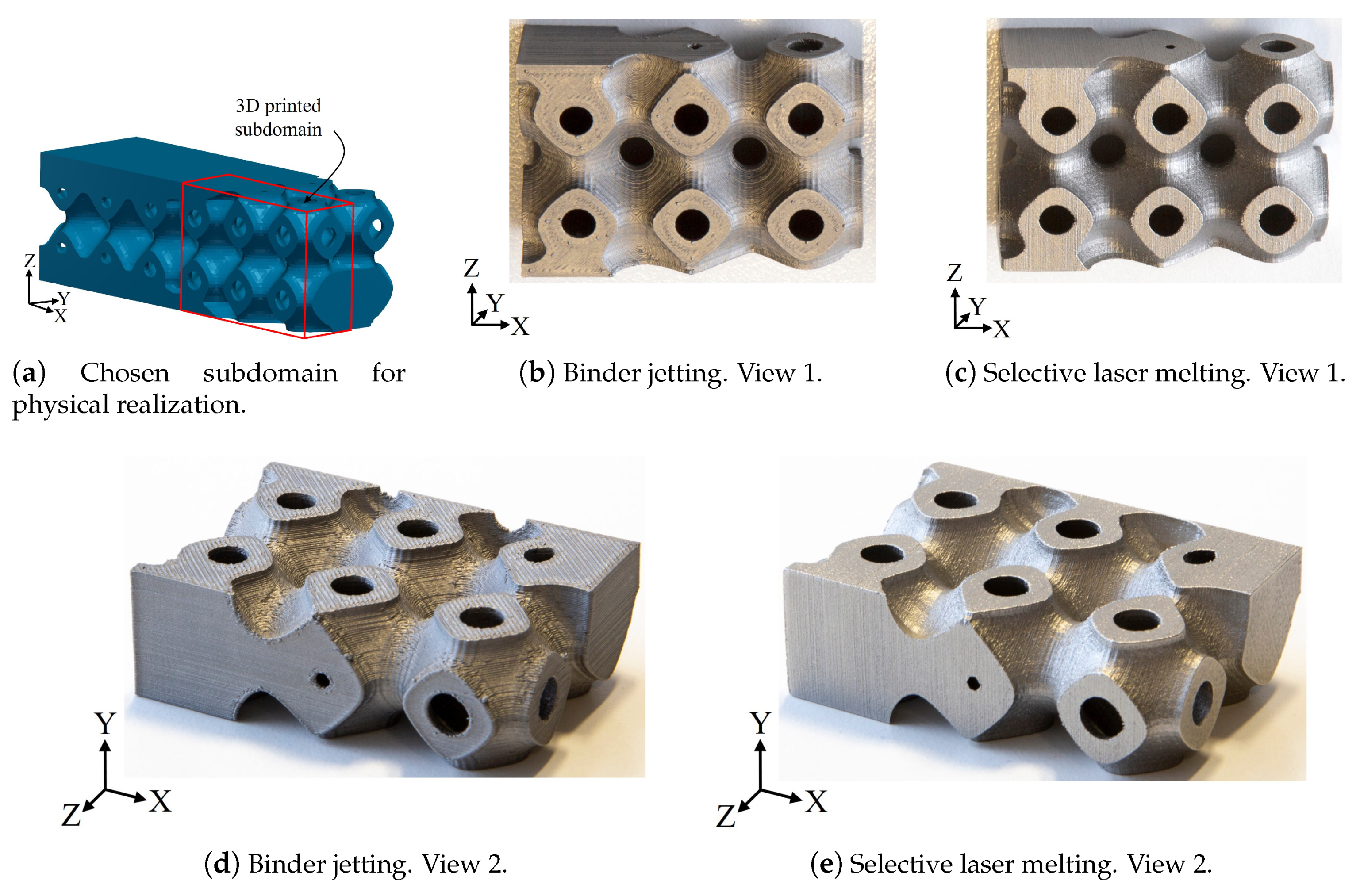
| Matrix-phase subdomain in Figure 14a | Figure 14b,d | 6 cm × 2 cm × 2 cm | Studio System (Desktop Metal) | Binder Jetting | 17–4PH stainless steel | 100 m | Y axis in Figure 14a | Yes | Debinding (12 h) Sintering (24 h) |
| Matrix-phase subdomain in Figure 14a | Figure 14c,e | 6 cm × 2 cm × 2 cm | Renishaw AM250 | Selective Laser Melting | 316L stainless steel | 100 m | X axis in Figure 14a | No | Stress relief (2 h) |
© 2019 by the authors. Licensee MDPI, Basel, Switzerland. This article is an open access article distributed under the terms and conditions of the Creative Commons Attribution (CC BY) license (http://creativecommons.org/licenses/by/4.0/).
Share and Cite
Montoya-Zapata, D.; Moreno, A.; Pareja-Corcho, J.; Posada, J.; Ruiz-Salguero, O. Density-Sensitive Implicit Functions Using Sub-Voxel Sampling in Additive Manufacturing. Metals 2019, 9, 1293. https://doi.org/10.3390/met9121293
Montoya-Zapata D, Moreno A, Pareja-Corcho J, Posada J, Ruiz-Salguero O. Density-Sensitive Implicit Functions Using Sub-Voxel Sampling in Additive Manufacturing. Metals. 2019; 9(12):1293. https://doi.org/10.3390/met9121293
Chicago/Turabian StyleMontoya-Zapata, Diego, Aitor Moreno, Juan Pareja-Corcho, Jorge Posada, and Oscar Ruiz-Salguero. 2019. "Density-Sensitive Implicit Functions Using Sub-Voxel Sampling in Additive Manufacturing" Metals 9, no. 12: 1293. https://doi.org/10.3390/met9121293
APA StyleMontoya-Zapata, D., Moreno, A., Pareja-Corcho, J., Posada, J., & Ruiz-Salguero, O. (2019). Density-Sensitive Implicit Functions Using Sub-Voxel Sampling in Additive Manufacturing. Metals, 9(12), 1293. https://doi.org/10.3390/met9121293