Article

Physical Modelling and Numerical Simulation of the Deep Drawing Process of a Box-Shaped Product Focused on Material Limits Determination

1
Faculty of Mechanical Engineering, Institute of Technology and Materials Engineering, Technical University of Košice, Mäsiarska 74, 040 01 Košice, Slovakia
2
Institute of Materials Research, Slovak Academy of Sciences, Watsonova 47, 040 01 Košice, Slovakia
*
Author to whom correspondence should be addressed.
Metals 2019, 9(10), 1058; https://doi.org/10.3390/met9101058
Submission received: 26 August 2019 / Revised: 25 September 2019 / Accepted: 26 September 2019 / Published: 28 September 2019
(This article belongs to the Special Issue Modelling and Simulation of Sheet Metal Forming Processes)

Abstract

:
Similitude theory helps engineers and scientists to accurately predict the behaviors of real systems through the application of scaling laws to the experimental results of a scale model related to the real system by similarity conditions. The theory was applied when studying the deep drawing process of a bathtub made from cold rolled low carbon aluminum-killed steel from the point of view of material limits. The bathtub model was created on the basis of geometric, physical, and mechanical similarity on a scale of 1:5. Thus, simulations and physical models were created. The simulation model was used to verify the combination yield locus/hardening law on the basis of comparing the thickness change. As a result, Hill 48/Krupkowski showed the minimal deviation by comparing data evaluated from numerical simulations and that measured on the physical model. Additionally, material anisotropy was modelled when virtual materials were defined from experimentally measured values of the plastic strain ratio. As an outcome, extra deep drawing quality steel with an average plastic strain ratio of rm ≥ 1.47 and an average strain hardening exponent of nm ≥ 0.23 must be used for the deep drawing of the bathtub.

1. Introduction

The deep-drawing process is widely used in automotive, transport, household, and other industries when metal sheets are processed. The optimization of process parameters, such as the blank shape, material, lubrication, gaps, drawbead dimensions, etc. requires good knowledge of the process and parameters influencing the quality of the drawn part [1]. Thus, the die design process for the drawing of stampings with complicated shapes is time- and cost-consuming due to testing of the concepts designed [2].
Manufacturing processes are tested either on physical models or by numerical simulations [3]. The real production process is difficult to test during its exploitation, so physical experiments are usually based on the scale model [4]. Similitude theory helps engineers or scientists to predict the behavior of a researched system through a scaled model. Langhaar [5] presented the general definition of similarity in mathematical terms for two functions. Szucs [6] widened the theory of similarity from functions to systems. Coutinho summarized the state-of-the-art knowledge on similitude theory and methodologies used to create reduced scale models, including those based on the use of dimensional analysis, differential equations, and energetic methods [7]. The theory of similarity and dimensional analysis in mechanics was also elaborated by Sedov [8].
Focusing on the metal forming processes, analysis of the similarity concept based on scaled model testing and dimensional analysis has taken place. Gronostajski proposed the plastic similarity condition for physical modelling of the axisymmetric backward extrusion of lead [9]. Davey introduced a novel scaling methodology using transport equations for the scaling of mass, momentum, energy, and entropy, as well as any associated material-constitutive relationships [10]. Al-Tamimi applied and validated the approach by means of scaled experimental and numerical and analytical solutions of scaled cold upsetting tests for cylindrical and ring samples for three trial materials [11]. Krishnamurthy applied the theory for the hot forging of the disk using numerical simulations of the real process and the scaled one. All the characteristics of the metal flow remained identical at all stages of the process [12]. Keran presented a study of the correlation between the workpiece size and forming force for a case of cylindrical body upsetting by using a numerical simulation. As a result, a difference of less than 3% compared with the results of the calculation using similarity theory was reached [13]. Ajiboye used the dimensional analysis based on the Buckingham π theorem for a sensitivity study of the frictional behavior in cold forging [14].
Accordingly, the deep drawing processes of the model need to be researched and designed under strictly defined conditions. The similarity criteria that must be considered when physically modelling the deep drawing process based on scaled models are
(a) the geometry similarity—the corresponding dimensions of the model and object have to be proportional; thus, the length scale factor is constant;
(b) the mechanical similarity—equal pressures, strain rates, press ram weights, and deformation works; and
(c) the physical similarity—the same material chemical composition, structure, temperature, friction, distribution of stress, strain, etc. [3,10,15].
Numerical simulations were used when designing the manufacturing processes in the 1990s to reduce time and costs. Silva utilized Pam-Stamp software to re-evaluate the stamping process for a rear seat and a structural reinforcement when changing the blank thickness and conventional steel to high strength steel [16]. Choudhury optimized the die geometry and determined the safe limit of the blankholder forces for plain carbon steel, reinforced steel, and aluminum alloy [17]. Padmanabhan numerically simulated the deep drawing process of bottles for LPG (bottled gas) by using DD3IMP FE code. The optimization of the variable blank holder force and friction condition at specific locations during deep drawing resulted in an increased minimum thickness in the deep drawn part [18]. Vafaeesefat proposed an algorithm to predict the initial blank shape from the desired part in the sheet metal forming process using LS-DYNA software [19]. Fracz used eta/Dynaform software when optimizing sheet metal forming of a cylindrical part made from AMS 5512 steel [20]. Čada used Dynaform software to evaluate the influences of the shape, size, and location of rectangular and semicircular draw beads on the sheet-metal forming process [21]. Labergere employed Abaqus software to propose and validate a global methodology to simulate the stamping of the embossed sheet and the capacity of the model to predict severe folds and the final shape of the part [22]. Using LS-Dyna software, Schrek researched the deep drawing process of tailor welded DP 600 and BH220 materials in tools with an elastic blankholder. They determined the values and points of application of the blankholder forces to achieve minimal movement of the weld interface [23].
As Roll presented in [15], it is important to describe material behavior and tribological factors in numerical simulations using proper mathematic models. This includes both yield loci definition and the hardening law. The use of the standard von Mises model to describe material behavior is not enough, and it needs to be widened to describe effects such as anisotropy and kinematic hardening. The problem is more emphasized when the simulation of springback is performed and new advanced high-strength steels or aluminum alloys are applied. Consequently, correct models for the material and friction coefficient must still be verified by experiments. Neto et al. numerically simulated the anisotropic behavior of the mild steel sheet used in the reverse deep drawing process of a cylindrical cup. The effect of the yield criterion on the numerical results was analyzed using three yield functions—von Mises, Hill’48, and Barlat Yld’91—combined with the Swift hardening law. The cup wall thickness distribution was strongly influenced by the yield criteria [24]. Other work by Neto et al. focused to the experimental and numerical analysis of a rail component made of mild steel and dual phase steel. They used the Swift hardening law to describe isotropic hardening and the Frederick–Armstrong law to describe the kinematic part of the work hardening combined with the Hill’48 yield criterion to describe the orthotropic plastic behavior of both metallic sheets. The results showed that the wrinkling behavior was strongly affected by the blank’s material as well as by the symmetry conditions (¼ of blank, full blank) defined in the numerical model [25]. Mulidran et al. focused on the springback prediction of a car body stamping made from aluminum alloy. The springback simulations were conducted with six yield functions (Barlat89, Barlat2000, Vegter-Lite, Hill90, Hill48 isotropic, and Hill48 orthotropic) combined with the Voce hardening model. Springback analysis was done in three sections, and the results were compared with the experimental values [26].
Chen researched the bathtub deep drawing process using numerical simulation [27]. It is supposed that he used the Hill isotropic definition of the yield locus and the point definition of the hardening curve. As a result, he determined an optimum drawbead distribution on the die face to avoid the formation of both fractures and wrinkles. Hojny [28] numerically simulated the stamping of the W1200 bathtub when the effects of the blank holder pressure and friction on the occurrence of fracture and wrinkling were investigated. He used the anisotropic Barlat model and point defined flow stress to define the material behavior.
In the article, numerical simulations based on the finite element method were performed to evaluate the influences of both the yield locus and the hardening law when deep drawing the model of box-shaped pressing—the bathtub model. The model pressing designed on the principle of similitude theory was numerically simulated for verification. The combination of the yield locus/hardening law was validated experimentally when compared with the thickness change in the selected sections. Simulations and experiments on the drawing quality of mild steel for enameling were performed, which is used in the production of real box-shaped pressing. Additionally, material anisotropy was modelled and verified using numerical simulation to determine the limit value from the point of view of fractures during deep drawing.

2. Materials and Methods

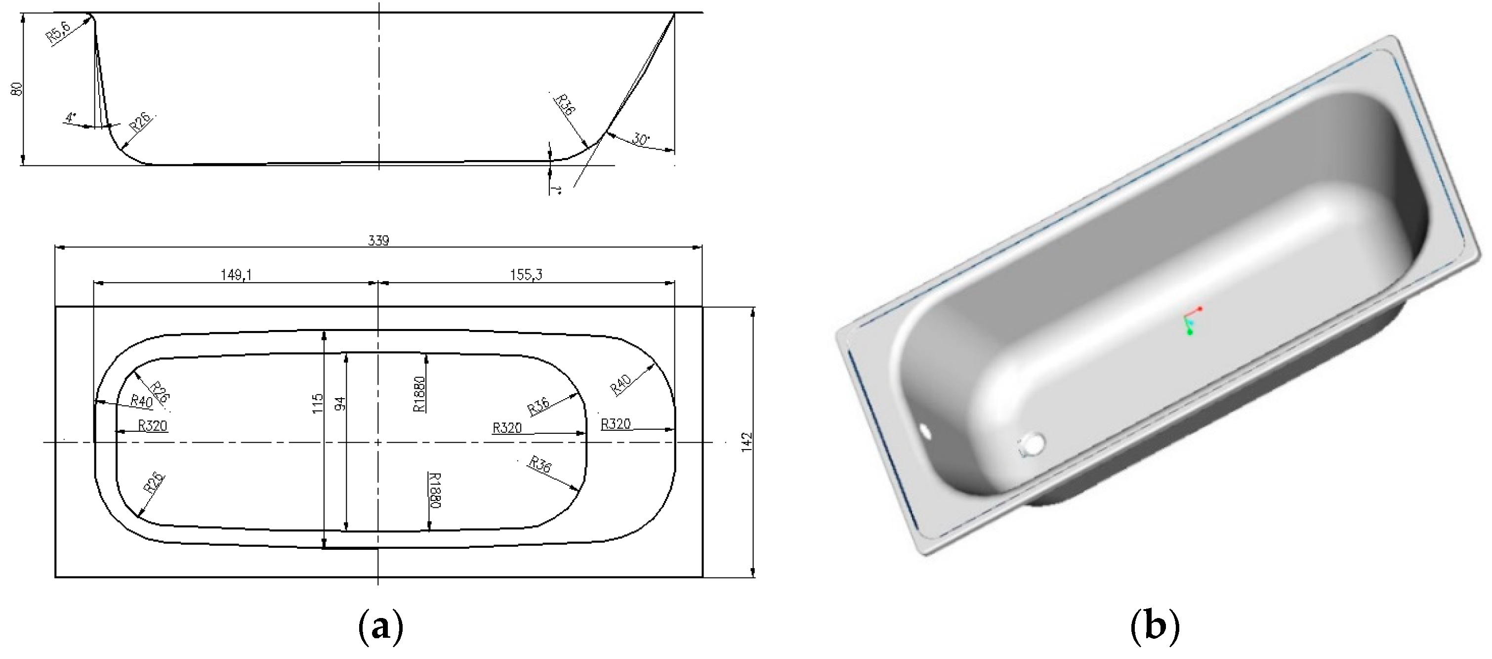
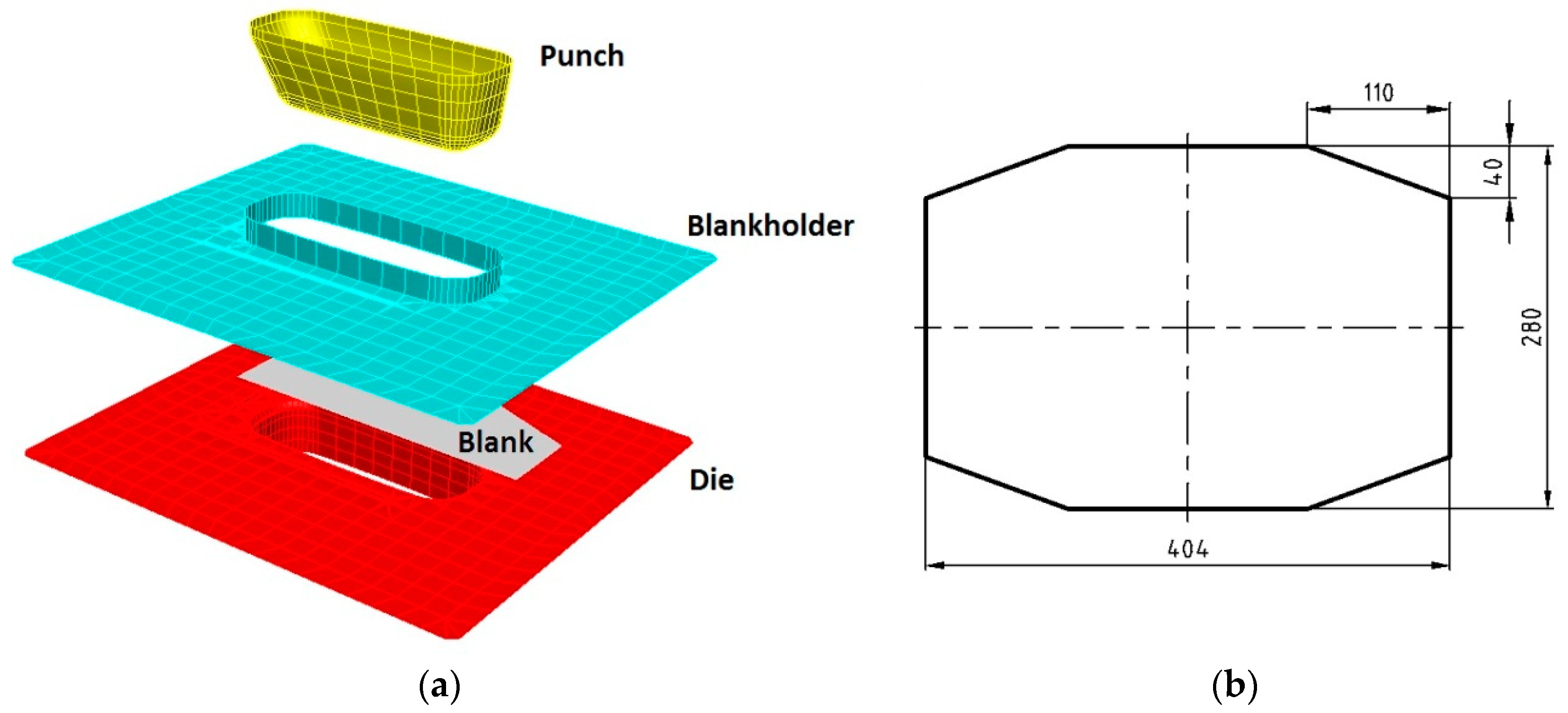
2.1. The Press-Die-Pressing System
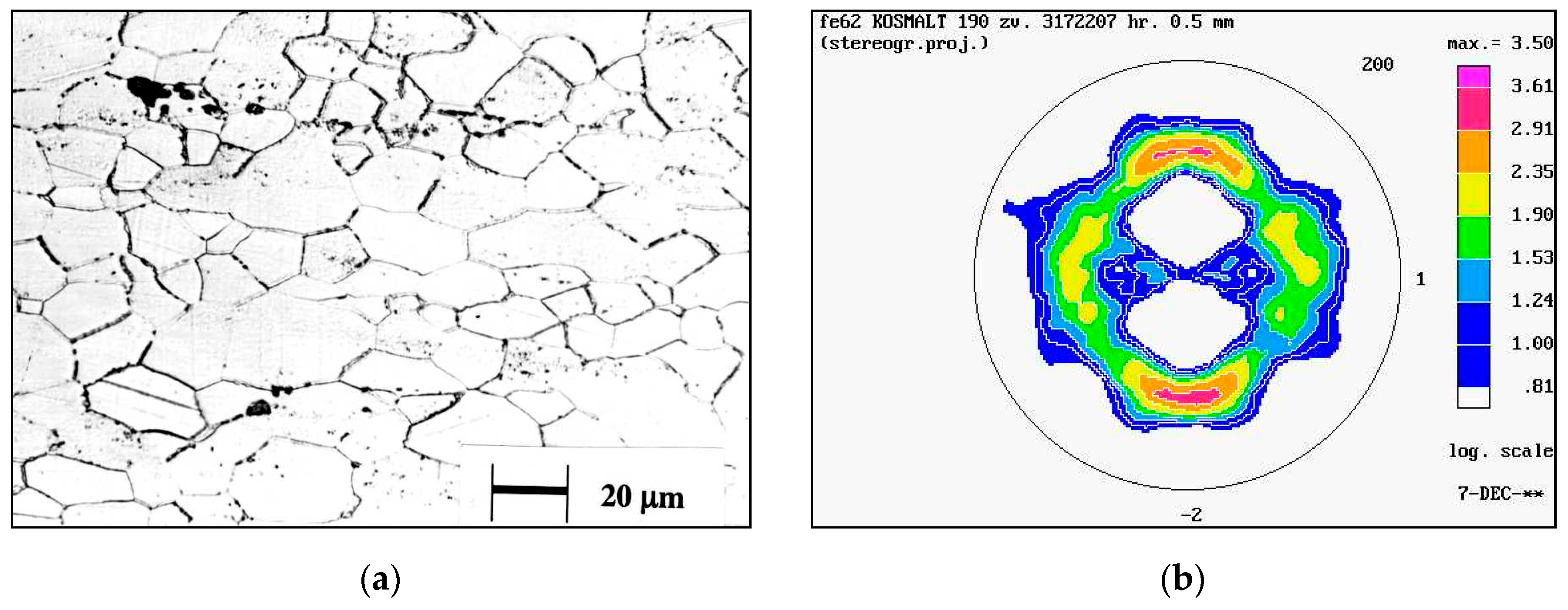
Bathtub model pressing was considered here as a box-shaped pressing. The model was designed according to similitude theory in order to verify the material parameters when deep drawing the real bathtub produced by Festap Ltd., Filakovo, Slovakia. The real bathtub pressing was scaled to the model (Figure 1) to meet the similarity criteria shown in Table 1. During real production, the steel sheet thickness decreases over the years from 2.5 to 1.63 mm; thus, the formability criteria of the material should be verified.
Based on the model dimensions and drawing die used for the real bathtub, the drawing die for the model pressing was designed. To reduce the material flow in the straight parts, drawbeads were used, and their positions, dimensions, and lengths were also scaled. An experimental drawing of the die is shown in Figure 2.

2.2. Material

The bathtubs used in the experiment were made from cold rolled steel sheet for enameling, which is produced by U.S. Steel Kosice. The deep drawing of the bathtub model was done using a Kosmalt 190 (i.e., DC06EK according to EN 10209) steel sheet with a thickness of 0.5 mm. This special steel had to meet two opposing requests: good formability and good enameling properties in the aspects of both the fishscale and the pinhole resistance. The steel belongs to a group of cold rolled low carbon aluminum-killed and annealed steel. This type of steel has a good hydrogen storage ability due to the numerous micro-voids generated after cold-rolling, which still exist after annealing [29]. The chemical composition of the steel is shown in Table 2; its microstructure and texture are shown in Figure 3.
The experimental material, Kosmalt 190, has a typical recrystallization structure. The density of the orientation components (111)<110> and (111)<112> is 10. The texture of the material is suitable for deep drawing. The structure is ferrite-pearlite-cementitic with a polyedric grain grade of 7 or occasionally grade 5. The cementite segregation is type 1A2, mainly on the grain boundaries in a few isolated cases in short rows.
For the numerical and physical experiments, Kosmalt 190 material with a nominal thickness of a0 = 0.5 mm was used. From the point of view of formability, the material properties are shown in Table 3. These were measured according to the following standards: mechanical properties by STN EN ISO 6892-1, the normal anisotropy ratio by STN EN ISO 10113, and the strain hardening exponent by STN EN ISO 10275 using the TIRAtest 2300 testing machine (TIRA Maschinenbau GmbH, Rauenstein, Germany) controlled by a PC.
Five specimens were measured in each rolling direction for each test. The elongation was measured by the length extensometer and the width reduction was measured by the width extensometer, both with a precision level of ±0.001 mm. The plastic strain ratio was calculated at the engineering strain level of 20% using automatic determination. The strain hardening exponent was evaluated within an engineering strain level of 5% to 20%. The average values and planar anisotropy were calculated as follows:
r m = 1 4 ( r 0 ° + 2 · r 45 ° + r 90 ° ) ,
Δ r = 1 2 ( r 0 ° 2 · r 45 ° + r 90 ° ) ,
n m = 1 4 ( n 0 ° + 2 · n 45 ° + n 90 ° ) ,
Δ n = 1 2 ( n 0 ° 2 · n 45 ° + n 90 ° ) .

2.3. Numerical Simulation Model

Numerical simulations were done using Pam-Stamp 2G software from the ESI Group (Paris, France). The simulation model was created using the 3D CAD/CAM software Creo, and its components were exported in neutral igs format. The die, punch, and blankholder were meshed using the Pam-Stamp 2G meshing module when importing CAD data. The meshed die components are shown in Figure 4a. To shorten the computing time, the symmetry of the blank along the longitudinal axis of the model was used. The blank shape (Figure 4b), dimensions, and its positioning against the die were also the same as for the real process and were scaled 1:5 to reach geometry similarity. The steel sheet rolling direction (0°) was positioned in the longitudinal axis of the bathtub model pressings.
There are two ways to represent drawing beads in a simulation model: (a) using a physical model—drawing beads need to be physically modelled on the CAD model of the blankholder and grooves on the die. This concept is a complicated way to simulate the blankholding stage individually before the drawing stage. Changing the restrictions on the bead geometry is complicated due to importation of a new blankholder model and meshing procedure; (b) using a numerical model—there is a macro within simulation software that can be used for drawbead action through restriction and the blankholing forces [27,30]. This property enables the actions of the drawbead on the blank and the blankholder to be represented without creating the geometry of the drawbead on the mesh. Thus, it is much easier to represent and modify a drawbead’s shape and dimensions. Drawbeads are represented by nodes and lines that are positioned against the die and the blankholder. Restriction and opening forces are calculated through the drawbead macro calculator with respect to its geometry. A simulation concept with a physical model of drawing beads was used, and its geometry (drawbead length, width, height, number, and position) was the same as the drawbead geometry of the experimental drawing die.
The validation meshing strategy was applied with a minimum element size of 0.1 and a maximum of 30, a chordal error of 0.15, and a maximum angle of 15° for radii and curved surfaces. Belytschko–Tsay shell 3-node and 4-node elements (triangles, squares, and rectangles) with the Gauss thickness integration rule were applied to the objects (punch, die, blankholder) and blank as well. The small radii on the drawbead and groove were meshed to six rectangular elements with a height of 0.25 mm; the die radius was meshed to six rectangular elements with a height of 1.45 mm. Both fulfilled the maximum angle of 15° between shells.
Because the size of blank mesh influences the results, it should be optimized to offer accurate results and the lowest time of calculation possible. Hence, an initial blank mesh size of 10 mm was applied along with the adaptive meshing strategy. This allowed the mesh size of the object in contact to be refined when necessary, especially in small radii on the drawbeads and the die. Thus, the refinement level was set to 5, and the final blank mesh size was 0.625 mm.

2.3.1. Material Hardening Model

Nowadays, different mathematical models are used to describe the plastic behavior of steel sheets: Hollomon (or Ludwik), Krupkowski (or Swift), Hocket‒Sherby, Gosh, Voce, Johnson‒Cook, Cowper‒Symonds etc. Some of these are strain rate and/or temperature dependent [30,31]. These were reached by fitting experimentally acquired data from tensile tests or other non-standardized tests, and they differ in terms of the effort required to calibrate the model and to reach the model’s constants. Two isotropic material hardening models were tested during the numerical simulation:
• Hollomon
σ = K · φ n
• Krupkowski
σ = K · ( φ 0 + φ p l ) n
where σ is the true stress, φ is the true strain, K is the strength coefficient, n is the strain hardening exponent, φ0 is the pre-strain, and φpl is the plastic strain.
The Hollomon hardening model was measured within the strain levels of 5% to 20%. The Krupkowski model was determined on the basis of Hollomon’s model parameters using the numerical iteration method. The models’ constants are shown in Table 4.

2.3.2. Material Yield Locus

The most important criterion in the numerical simulation is the yield locus, which describes the transition from an elastic state to a plastic one. The yield locus also expresses the relationships between stress components at the moment of yielding due to the multiaxial stress state during metal forming. Thus, the yield point measured during uniaxial tension in the tensile test is not enough to describe the yield locus even if it is easily measured. [32]
The most widely used yield criteria for isotropic materials are Tresca (the “maximum shear stress criterion”) and von-Mises (the “strain energy criterion”). However, the sheet metal exhibits a significant anisotropic property due to its crystallographic structure and the characteristics of the rolling process. Hence, in 1948, Hill [33] proposed an anisotropic yield criterion involving three orthogonal symmetry planes, which is expressed by the following quadratic function:
2 f ( σ i j ) = F ( σ y σ z ) 2 + G ( σ z σ x ) 2 + H ( σ x σ y ) 2 + 2 L τ y z 2 + 2 M τ z x 2 + 2 N τ x y 2 = 1 ,
where F, G, H, L, M, and N are constants specific to the anisotropy state of the material, and x, y, and z are the principal anisotropy axes [30,33]. Because the plane stress is assumed in numerical simulations of the sheet metal forming processes, the stress in the thickness direction is ignored due to its insignificance compared with that in the other two orthogonal directions. Furthermore, assuming that the principal directions of the stress tensor are coincident with the anisotropic axes, this criterion can be written as follows:
σ 1 2 2 r 0 1 + r 0 σ 1 σ 2 + r 0 ( 1 + r 90 ) r 90 ( 1 + r 0 ) σ 2 2 = σ 0 2 .
In 1990, Hill stated that the range of validity of Hill 48 had been explored through numerous experiments, and that it is well suited to specific metals and textures. For more recently developed steels of higher grades, Hill 90 was developed [34]. This is a yield criterion for metal sheets with planar anisotropy, and it is based on a non-quadratic yield function. This criterion takes into account different behaviors during the bending/unbending phase. The model is a generalization of Hill 48 with non-integer powers of the principal values of the deviatoric stresses. Its constitutive relation for plane stress conditions in terms of principal stress components can be written as follows: [30,34]
| σ 1 + σ 2 | m + α · | σ 1 σ 2 | m + | σ 1 2 σ 2 2 | m 2 1 · c o s ( 2 Φ ) [ β · ( σ 1 2 σ 2 2 ) + γ · ( σ 1 σ 2 ) 2 · c o s ( 2 Φ ) ] = 2 · σ Y m ,
where α, β, γ, and m are constants derived from the measured material data, Φ is the angle between the principal axes of the in-plane stress and the principal axes of anisotropy, and σY is the equi-biaxial yield stress.
The Hill 48 yield locus was defined by Lankford’s coefficients r0, r45, r90 (i.e., plastic strain ratios), and these were measured using tensile tests performed on the specimens taken at 0°, 45°, and 90° to the rolling direction (see Table 3).
To calculate the coefficients α, β, γ, and m for the Hill 90 yield locus, the Pam-Stamp 2G wizard was used. This calculation is based on an iterative method that minimizes a function whose variables are the yield stresses and the anisotropy coefficients (least-squares method). The user must define the uniaxial yield values Rp0.2 for each Lankford’s coefficient rα and either the Hill 90 coefficient m or the equi-biaxial yield stress σy. An equi-biaxial yield stress of σy = 220 MPa was used for the calculations, which was obtained from a hydraulic bulge test using the HYDROTEST device. Uniaxial yield values Rp0.2 and Lankford’s coefficients for the rolling directions of 15°, 30°, 60°, and 75° were additionally tested according to standards shown previously (Table 5). The values of the Hill 90 yield locus constants α, β, γ, and m are shown in Table 6.

2.3.3. Failure Criteria

Keeler-Brazier’s model of forming limit curve was used to determine the material fracture in a numerical simulation. The model was implemented in Pam-Stamp 2G software, and the value of φ1 when φ2 = 0 was calculated as follows: [30,35]
φ 1 ( 0 ) = ln [ 1 + ( 23.3 + 14.13 a 0 ) n 0.21 ]
when   φ 2   <   0   φ 1 = φ 1 ( 0 ) φ 2
when   φ 2   >   0   φ 1 = φ 1 ( 0 ) + 0.6 [ exp ( φ 2 1 ) ]
where a0 is the material thickness, and n is the strain hardening exponent. The left side of the FLC curve was calculated from Equation (11) and the right side from Equation (12).

2.3.4. Boundary Conditions
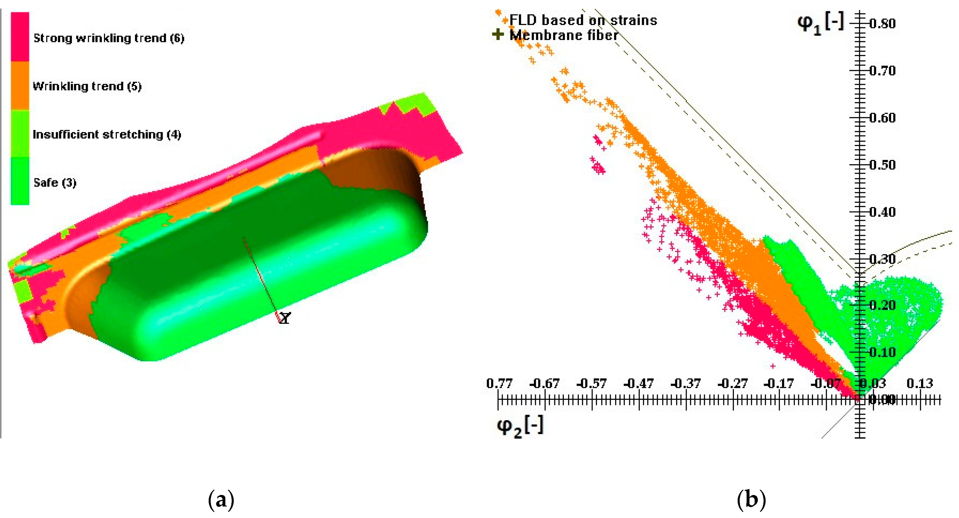
To perform numerical simulations, other boundary conditions or process parameters such as the blankholder force, friction, punch speed, and blankholder speed needed to be defined. Based on recommendations in the software manual, the blankholder speed was set to 2 m·s−1, and the punch speed was set to 5 m·s−1. In the z direction, both increased linearly from zero to the final value to prevent dynamic effects at contact. This was defined as the imposed velocity by the curve [30]. Contact conditions were defined by the friction coefficient and the Coulomb laws defined the friction. Water-based lubricant is used when real bathtubs are produced, so the friction coefficient was set to a constant value of 0.09 due to the friction between the steel sheet and tool steel [28,36]. The blankholder force was set to 340 kN when the bathtub model pressing free of wrinkles and fracture was drawn.

3. Results

Within the numerical simulations, each hardening model was combined with each yield criterion. Overall, four simulation concepts were done by changing the material hardening law and the yield locus. These combinations are shown in Table 7.
Qualitative evaluation of the numerical simulations was done using the FLD diagram in order to evaluate the deep drawing process from the point of view of both the wrinkles appearance and fracture. In all simulation concepts, fracture did not occur, while a wrinkle tendency was identified in the same areas. However, on the physical model, wrinkles were not identified. The result for simulation 2 is shown in Figure 5. The material is appeared to have very good formability, as shown by the value of the strain hardening exponent and the plastic strain ratios presented in Table 3.
To validate the material hardening law/yield locus combination, the wall thickness change was evaluated in selected sections. The sections used to measure the wall thickness change are shown in Figure 6. On the bathtub model pressing reached by the physical experiment, the thickness was measured using a micrometer (conical tips with flat spot of Ø 1 mm) three times at a single point, and the average thickness value was calculated. There was a distance of 5 mm between measurement points along the bathtub wall’s length.
The minimal thicknesses for the individual simulations and measured on the physical model are shown in Table 7. The minimal thickness was identified in the G-H area in the longitudinal section A-A for each simulation, i.e., at the radius of the inclined wall to the bottom. The second minimal thickness was identified in the D-E area, i.e., at the radius of the wall to the bottom for Hill 48 yield locus, but in the C-D area, i.e., at the wall, for Hill 90 yield locus. The minimal thickness in section B-B was found in the D-E area too. There was good agreement between the numerical simulation and the real measurement of thickness for each simulation representing the material hardening law/yield locus combination when considering the minimum thickness position. A comparison of the relative thickness change evaluated from the numerical simulations and measured on the bathtub model pressing is shown in Figure 7.
To assess the hardening law/yield locus combination, the deviation of the thickness evaluated from the numerical simulation and measured on the physical model was calculated as follows:
Dev = ( Th simul Th real ) Th nom · 100 [ % ]
where Thsimul is the thickness evaluated from the numerical simulation, Threal is the thickness measured on the physical model, and Thnom is the nominal steel sheet thickness. The results are shown in Table 8 and in Figure 8. Based on the evaluation using the minimal thickness criterion, the best combination seems to be the Hill 48 yield locus and the Krupkowski material hardening law. The values of thickness at both critical regions were the closest to the thicknesses measured on the bathtub model pressing. The graph on Figure 8 shows the deviation of thickness evaluated from the numerical simulation and the thickness measured on the bathtub model pressing for each combination material hardening law/yield locus.
As mentioned previously, enameling steel must meet two opposing requests: good drawability and good enameling properties. Steel used in the physical experiment and numerical simulation belongs to the group of cold rolled low carbon aluminum-killed and annealed steel. From the point of view of drawability, this steel shows anisotropy due to its production process [37]. Thus, the effect of anisotropy was researched by numerical simulation to determine the minimal values when pressing free of fracture was reached in the model.
Based on the material properties shown in Table 3, other two materials were modelled from the point of view of its anisotropy. Directional values of plastic strain ratios were lowered, as shown in Table 9: about 0.1 in the rolling direction, about 0.05 at 45°, and about 0.2 at 90°. The differences in each direction were chosen on the basis of the formability evaluation of different grades of Kosmalt steel sheet, as presented in [37]. Then, the deep drawing process was numerically simulated, and the results are shown in Figure 9 and Figure 10.
When analyzing the results, the critical area of the bathtub model pressings was found to be the bottom radii at the corner. Thus, localized necking or fracture occurred when the plastic strain ratios were lowered in the 0°, 45°, and 90° directions. Considering the blank positioning (rolling direction of 0° in the longitudinal axis) and the directional dependence of the plastic strain ratio, i.e., its anisotropy, it is the location of r45 where the lowest value was measured. The results comply with those of [37], because the plastic strain ratio expresses the steel sheet’s resistance to thinning. Thus, greater thinning of the thickness appears in the direction of the lowest plastic strain ratio.

4. Discussion

Previously published research on the bathtub deep drawing process by numerical simulation was focused on determining an optimum drawbead distribution on the die face [27] and the effects of the blankholder pressure and friction on the occurrence of fracture and wrinkling [28], but the material model definition was not clear. The bathtub model deep drawing process was researched in the presented study from the point of view of, firstly, mathematic modelling of the yield locus and the hardening law and, secondly, modelling the material anisotropy limit.
The bathtub model deep drawing process was designed to reach geometric and physical similarity by using scaled modelling die and the same material, deformation process, and friction characteristics [7,9,10,11,12,13]. Thus, the Buckingham π theorem was applied and a physical model of the drawing die was designed at a scale of 1:5. Consequently, the simulation model was defined in PamStamp 2G software when the friction was set to 0.09 [30,36] and the blankholder force was 340 kN (the specific blankholder pressure was 6 MPa) to reach a model pressing free of wrinkles and fractures.
Because special steel for enameling is used for the production of bathtubs, four simulations were done to verify the combination yield locus/hardening law. It is desirable to note that the hardening curves described in Equations (5) and (6) are consistent with experimental ones only at a certain strain stage, and with large strains, the flow curve reaches saturation [38]. Thus, necking and fracture were judged by a forming limit curve [39]. Concerning the yield locus, both anisotropic criteria came from directionally measured plastic strain ratios, while Hill 48 is well adapted for strongly anisotropic materials (r > 1) and Hill 90 is used for materials with planar anisotropy (r < 1) [40]. The validity of the combination yield locus/hardening law was judged by comparing the thickness change in selected sections [16,18,20]. As a result, the Hill 48 yield locus combined with the Krupkowski hardening law offered the lowest thickness deviation (2.4%) when values calculated from numerical simulations and the physical model were compared. The results comply with [24] and were also used for mild steel and drawing quality steel when the deep drawing process was numerically simulated [16,17,21,25]. The selection of a proper mathematical model for the yield locus and hardening law is even more important for metal sheets and processes, especially when new types of steel or springback phenomena are simulated [17,25,26]. To define these models, more tests than just measuring uniaxial tension with a tensile test or biaxial tension with the Bulge test are necessary [15,32].
Keeler‒Brazier’s model determined the fracture limit and necking (marginal zone) in numerical simulations. Because it outcomes from a large number of experiments, it is well adopted in the numerical simulation of low carbon steels. It is easy to define using the strain hardening exponent and the thickness of material, while both influence the formability of the material [41,42,43]. However, constant strain paths are required during deep drawing, and their linearity was confirmed using software. This is also supported by the fact that the strain pathways in the first drawing of axisymmetric and uniform sectioned parts are satisfactorily linear, and the FLD for the as-received condition can be used comfortably when making formability assessments [39].
As an outcome of numerical simulations done for virtual materials, cold rolled low carbon aluminum-killed steel used for enameling must meet the conditions of rm ≥ 1.47 and nm ≥ 0.23 to obtain bathtub model pressings free of fracture. To improve the deep drawing process of the bathtub model pressing or the real bathtub in production, it is recommended that these values are higher. This is because the plastic strain ratio improves the steel sheet’s resistance to thinning of the thickness, while the strain hardening exponent unifies the strain distribution during deformation and prevents necking [37].
To improve the drawability, new steels have been developed such as ultra-low carbon Ti-IF steel, decarbonized (De-C) steel [29], and boron-microalloyed steel [44,45]. These possess excellent deep drawability with a lower yield stress and a higher elongation, plastic strain ratio, and strain hardening exponent compared with those of low carbon Al-killed steels. For Ti-IF and De-C steel, this is because of the very low carbon component when Ti is added, which stabilizes all of the carbon and nitrogen atoms, eliminates ageing, and improves elongation in the rolling direction [29,44,45,46]. Modern ideas to improve the ductility and preserve the high strength of sheet metal for deep drawing lies in the use of materials with ultrafine grained structures when complemented with coarse grained elements [47].

5. Conclusions

The bathtub model deep drawing process was researched in the presented study from the point of view of, firstly, mathematic modelling of the yield locus and hardening law and, secondly, modelling of the material anisotropy limit. Based on the numerical simulations and physical experiment performed, the following outputs can be concluded:
  • The Hill 48 and Hill 90 yield locus mathematical models and the Hollomon and Krupkowski hardening law mathematical models for cold rolled low carbon aluminum-killed steel for enameling were determined from tensile tests at angles of 0°, 45°, and 90° to the rolling direction and bulge tests. Experimental Kosmalt 190 steel with a thickness of a0 = 0.5 mm showed extra deep drawing quality with rm = 1.57 and nm = 0.226.
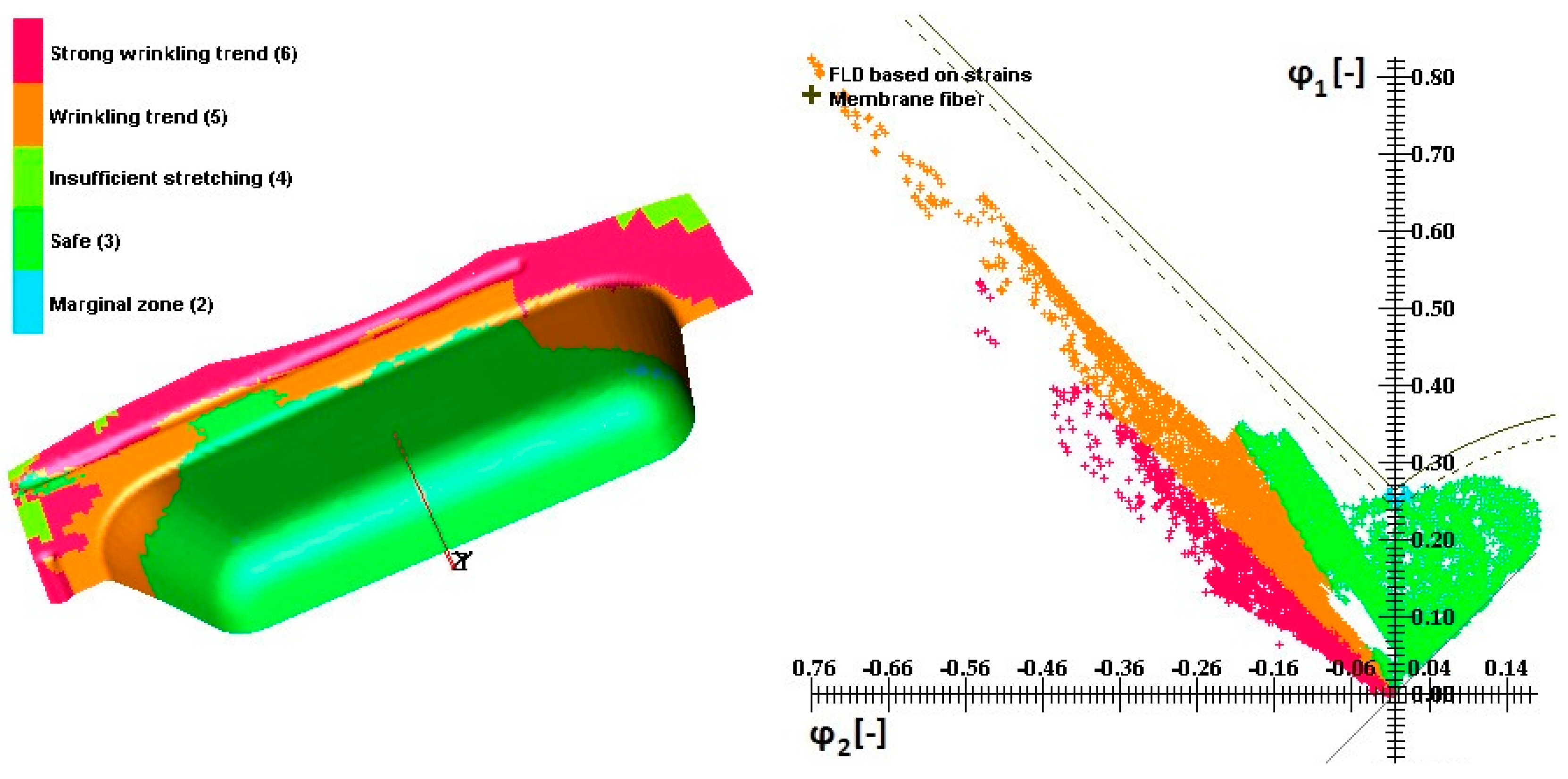
  • In all numerical simulations and physical experiments, the bathtub model pressing was drawn free of fracture and wrinkles when simulated at the same blankholder force (340 kN) and friction (0.09) values. Keeler-Brazier’s mathematic model was used to define the forming limit curve and to determine material fracture in numerical simulations.
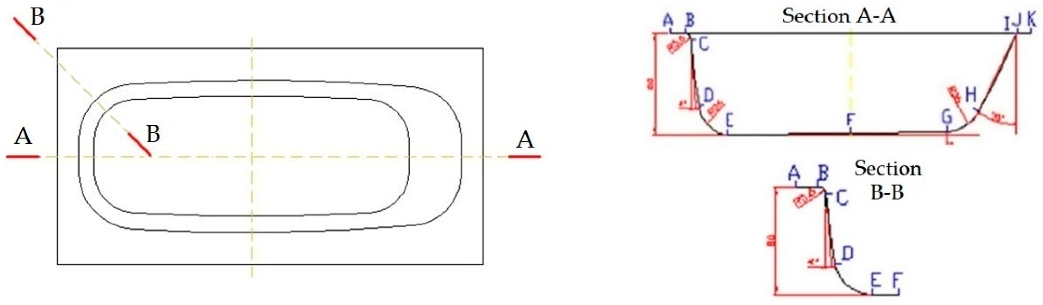
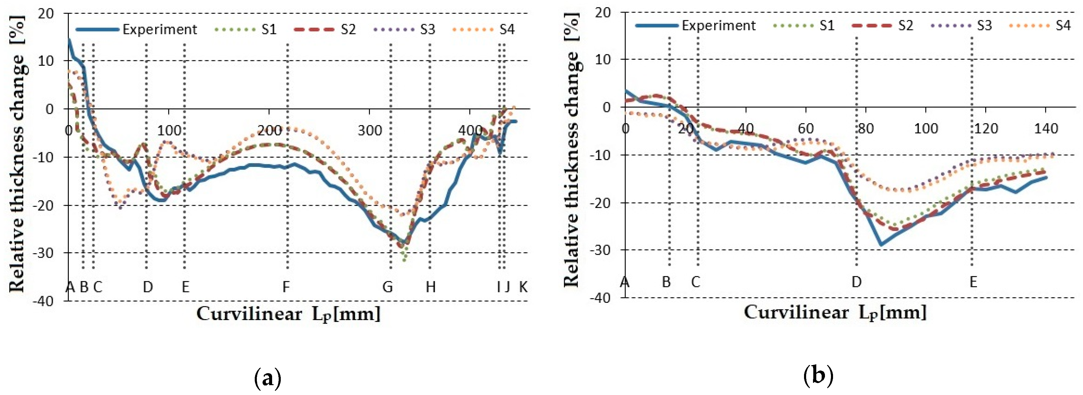
  • The best yield locus/hardening law combination appeared to be Hill 48/Krupkowski. This was determined by comparing the wall thicknesses of model pressing in selected sections after simulations and physical experiments. The deviations at the local minima were 0.7% and −1.0% in section A-A (longitudinal) and 2.4% in section B-B (corner). The course of relative thickness change evaluated from numerical simulations and experimental measurements showed good conformity.
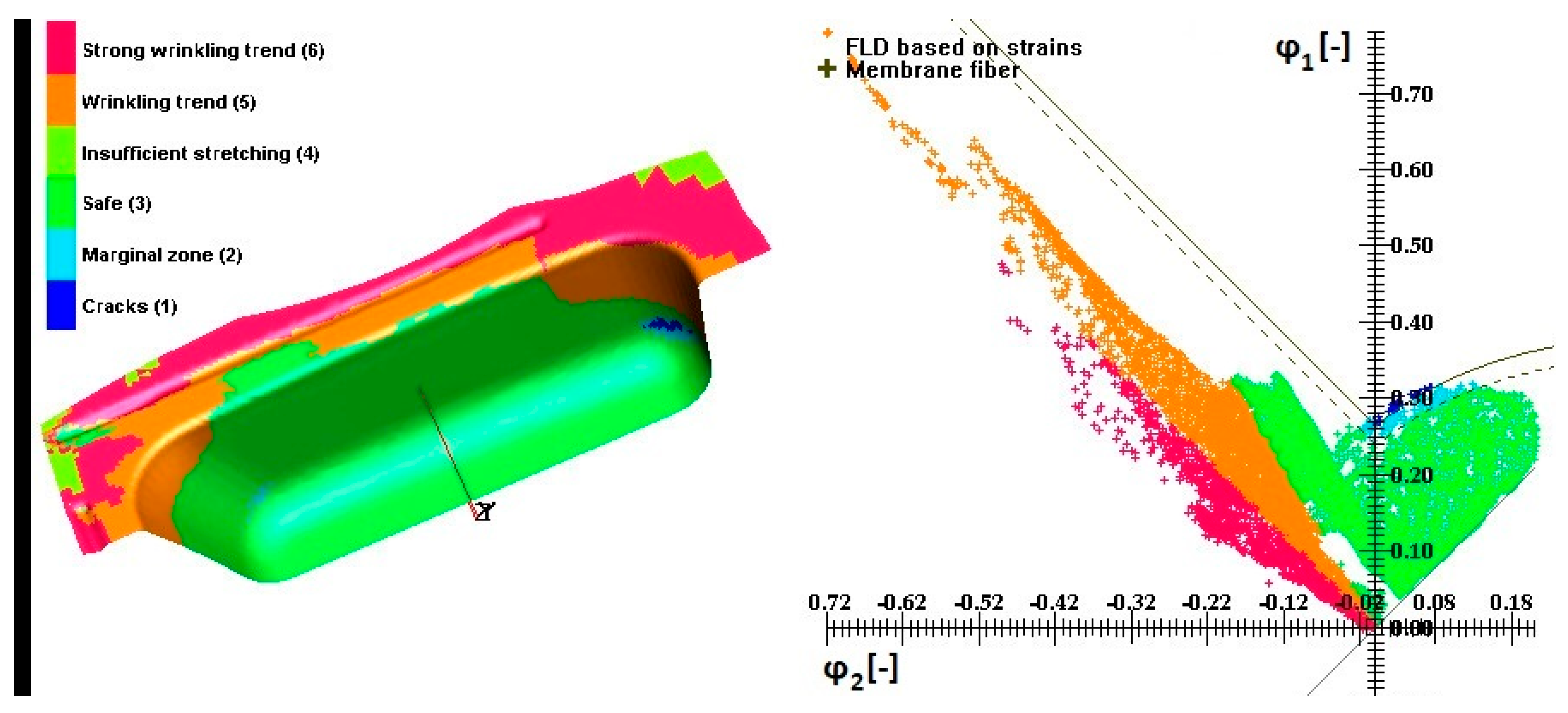
  • The material’s anisotropy limits were found to be rm = 1.47 and nm = 0.23 when the model pressing free of fracture was drawn in a numerical simulation. Virtual materials were defined from experimentally measured values of the plastic strain ratio.

Author Contributions

M.T. and E.E. designed the experiment; M.T. and J.K. performed and evaluated the numerical simulations; M.T. and J.H. designed the model die and performed and evaluated the physical experiment; M.T., E.E., J.K., and J.H. analyzed the results; M.T. wrote the article.

Funding

This research received no external funding.

Acknowledgments

The work was accomplished under the grant project VEGA 2-0080-19 “Prediction of weldability and formability for laser welded tailored blanks made of combined high strength steels with CAE support” and project APVV-0273-12 “Supporting innovations of autobody components from the steel sheet blanks oriented to the safety, the ecology and the car weight reduction”.

Conflicts of Interest

The authors declare no conflict of interest.

References

  1. Menezes, L.F.; Teodosiu, C. Three-dimensional numerical simulation of the deep-drawing process using solid finite elements. J. Mater. Process. Technol. 2000, 97, 100–106. [Google Scholar] [Green Version]
  2. Thomas, W.; Oenoki, T.; Altan, T. Process simulation in stamping—Recent applications for product and process design. J. Mater. Process. Technol. 2000, 98, 232–243. [Google Scholar] [CrossRef]
  3. Spišák, E. Mathematical Modelling and Simulation of Technological Processes—Deep Drawing, 1st ed.; ELFA, Ltd.: Košice, Slovakia, 2000; p. 156. ISBN 80-7099-530-0. [Google Scholar]
  4. Jha, A.; Sedaghati, R.; Bhat, R. Dynamic Testing of Structures Using Scale Models. In Proceedings of the 46th AIAA/ASME/ASCE/AHS/ASC Structures, Structural Dynamics & Materials Conference, Austin, TX, USA, 18–21 April 2005; AIAA 2005-2259. American Institute of Aeronautics and Astronautics: Reston, VA, USA, 2005. [Google Scholar] [Green Version]
  5. Langhaar, H.L. Dimensional Analysis and Theory of Models, 1st ed.; John Wiley & Sons: New York, NY, USA, 1951; ISBN 9780471516781. [Google Scholar]
  6. Szucz, E. Similitude and Modeling: Fundamental Studies in Engineering, 1st ed.; Elsevier: Amsterdam, The Netherlands, 1980; Volume 2. [Google Scholar]
  7. Coutinho, C.P.; Baptista, A.J.; Rodrigues, J.D. Reduced scale models based on similitude theory: A review up to 2015. Eng. Struct. 2016, 119, 81–94. [Google Scholar] [CrossRef]
  8. Sedov, L.I. Similarity and Dimensional Methods in Mechanics, 10th ed.; CRC Press: Boca Raton, FL, USA, 1993; p. 496. ISBN 9780849393082. [Google Scholar]
  9. Gronostajski, Z.; Hawryluk, M. Analysis of metal forming processes by using physical modeling and new plastic similarity condition. In Proceedings of the CP907, 10th ESAFORM Conference on Material Forming, Zaragoza, Spain, 18–20 April 2007. [Google Scholar]
  10. Davey, K.; Darvizeh, R.; Al-Tamimi, A. Finite Similitude in Metal Forming. In Proceedings of the NUMIFORM 2016: The 12th International Conference on Numerical Methods in Industrial Forming, Troyes, France, 4–7 July 2016. [Google Scholar]
  11. Al-Tamimi, A.; Darvizeh, R.; Davey, K. Experimental investigation into finite similitude for metal forming processes. J. Mater. Process. Technol. 2018, 262, 622–637. [Google Scholar] [CrossRef]
  12. Krishnamurthy, B.; Bylya, O.; Davey, K. Physical modelling for metal forming processes. Procedia Eng. 2017, 207, 1075–1080. [Google Scholar] [CrossRef]
  13. Keran, Z.; Piljek, P.; Ciglar, D. Metal forming similarity theory in numerical simulations. J. Technol. Plast. 2016, 41, 38–45. [Google Scholar]
  14. Ajiboye, J.S.; Jung, K.H.; Im, Y.T. Sensitivity study of frictional behavior by dimensional analysis in cold forging. J. Mech. Sci. Technol. 2010, 24, 115–118. [Google Scholar] [CrossRef]
  15. Roll, K. Simulation of sheet metal forming—Necessary developments in the future. In Proceedings of the NUMISHEET, 7th International Conference on Numerical Simulation of 3D Sheet Metal Forming Processes, Interlaken, Switzerland, 1–5 September 2008; ETH Zürich: Zürich, Switzerland, 2008; pp. 3–11. [Google Scholar]
  16. Silva, M.B.; Baptista, R.M.S.O.; Martins, P.A.F. Stamping of automotive components: A numerical and experimental investigation. J. Mater. Process. Technol. 2004, 155, 1489–1496. [Google Scholar] [CrossRef]
  17. Choudhury, I.A.; Lai, O.H.; Wong, L.T. PAM-STAMP in the simulation of stamping process of an automotive component. Simul. Model. Pract. Theory 2006, 14, 71–81. [Google Scholar] [CrossRef]
  18. Padmanabhan, R.; Oliveira, M.C.; Alves, J.L.; Menezes, L.F. Numerical simulation and analysis on the deep drawing of LPG bottles. J. Mater. Process. Technol. 2008, 200, 416–423. [Google Scholar] [CrossRef] [Green Version]
  19. Vafaeesefat, A. Finite Element Simulation for Blank Shape Optimization in Sheet Metal Forming. Mater. Manuf. Process. 2011, 26, 93–98. [Google Scholar] [CrossRef]
  20. Frącz, W.; Stachowicz, F.; Pieja, T. Aspects of verification and optimization of sheet metal numerical simulations process using the photogrammetric system. Acta Metall. Slovaca 2013, 19, 51–59. [Google Scholar] [CrossRef]
  21. Čada, R.; Tiller, P. Evaluation of Draw Beads Influence on Intricate Shape Stamping Drawing Process. Technol. Eng. 2014, 11, 5–10. [Google Scholar] [CrossRef] [Green Version]
  22. Labergere, C.; Badreddine, H.; Msolli, S.; Saanouni, K.; Martiny, M.; Choquart, F. Modeling and numerical simulation of AA1050-O embossed sheet metal stamping. Procedia Eng. 2017, 207, 72–77. [Google Scholar] [CrossRef]
  23. Schrek, A.; Švec, P.; Brusilová, A.; Gábrišová, Z. Simulation process deep drawing of tailor welded blanks DP600 and BH220 materials in tool with elastic blankholder. J. Mech. Eng. Stroj. Caopis 2018, 68, 95–102. [Google Scholar] [CrossRef]
  24. Neto, D.M.; Oliveira, M.C.; Alves, J.L.; Menezes, L.F. Influence of the plastic anisotropy modelling in the reverse deep drawing process simulation. Mater. Des. 2014, 60, 368–379. [Google Scholar] [CrossRef]
  25. Neto, D.M.; Oliveira, M.C.; Santos, A.D.; Alves, J.L.; Menezes, L.F. Influence of boundary conditions on the prediction of springback and wrinkling in sheet metal forming. Int. J. Mech. Sci. 2017, 122, 244–254. [Google Scholar] [CrossRef] [Green Version]
  26. Mulidran, P.; Šiser, M.; Slota, J.; Spišák, E.; Sleziak, T. Numerical Prediction of Forming Car Body Parts with Emphasis on Springback. Metals 2018, 8, 435. [Google Scholar] [CrossRef]
  27. Chen, F.K.; Chiang, B.H. Analysis of die design for the stamping of a bathtub. J. Mater. Process. Technol. 1997, 72, 421–428. [Google Scholar] [CrossRef]
  28. Hojny, J.; Wozniak, D.; Glowacki, M.; Zaba, K.; Nowosielski, M.; Kwiatkowski, M. Analysis of die design for the stamping of a bathtub. Arch. Metall. Mater. 2015, 60, 661–666. [Google Scholar] [CrossRef]
  29. Sun, Q.; Xu, C.; Jiang, W. Study on the enameling properties of cold-rolled sheet steels containing different alloyed elements. Glass Enamel 2015, 6, 1–5. [Google Scholar]
  30. ESI Group. Pam-Stamp 2015 User’s Guide; ESI Group: Paris, France, 2015. [Google Scholar]
  31. Gerlach, J.; Kessler, L.; Linnepe, M. A study regarding material aspects for numerical modelling of mild steels. In Proceedings of the IDDRG 2009 Conference—Material Property Data for More Effective Numerical Analysis, Golden, CO, USA, 1–3 June 2009; pp. 351–360. [Google Scholar]
  32. Wang, L.; Lee, T.C. The effect of yield criteria on the forming limit curve prediction and the deep drawing process simulation. Int. J. Mach. Tools Manuf. 2006, 46, 988–995. [Google Scholar] [CrossRef]
  33. Hill, R.A. Theory of the yielding and plastic flow of anisotropic metals. Proc. R. Soc. Lond. Ser. A Math. Phys. Sci. 1948, 193, 281–297. [Google Scholar]
  34. Hill, R. Constitutive modelling of orthotropic plasticity in sheet metals. J. Mech. Phys. Solids 1990, 38, 405–417. [Google Scholar] [CrossRef]
  35. Keeler, S.P.; Brazier, W.G. Relationship between Laboratory Material Characterization and Press-Shop Formability. Microalloying 1975, 75, 517–530. [Google Scholar]
  36. Hrivňák, A.; Evin, E. Formability of Steels, 1st ed.; Elfa: Košice, Slovakia, 2004; ISBN 80-89066-93-3. [Google Scholar]
  37. Pollák, L.; Tomáš, M.; Kuzmišin, J. Material formability and anisotropy of steel sheets for enamelling. In Proceedings of the 2005 International Scientific Conference on Structural Materials, Trnava, Slovakia, 22 June 2005; STU Bratislava: Bratislava, Slovakia, 2005; pp. 1–9. [Google Scholar]
  38. Beygelzimer, Y.; Kulagin, R.; Toth, L.S.; Ivanisenko, Y. The self-similarity theory of high pressure torsion. Beilstein, J. Nanotechnol. 2016, 7, 1267–1277. [Google Scholar] [CrossRef] [Green Version]
  39. Paul, S.K. Path independent limiting criteria in sheet metal forming. J. Manuf. Process. 2015, 20, 291–303. [Google Scholar] [CrossRef]
  40. Koc, M. Hydroforming for Advanced Manufacturing, 1st ed.; Woodhead Publishing: Amsterdam, The Netherlands, 2008; ISBN 9781845693282. [Google Scholar]
  41. Banabic, D. Sheet Metal. Forming Processes—Constitutive Modelling and Numerical Simulation, 1st ed.; Springer: Berlin/Heidelberg, Germany, 2010. [Google Scholar]
  42. Shaw, J.; Chen, M.; Watanabe, K. Metal Forming Characterization and Simulation of Advanced High Strength Steels. SAE Trans. 2001, 110, 926–935. [Google Scholar]
  43. Tisza, M.; Kovácx, Z.P. New methods for predicting the formability of sheet metals. Prod. Process. Syst. 2012, 5, 45–54. [Google Scholar]
  44. Denes, E.; Gergely, J.; Szabados, O.; Vero, B. A Comparative Study of the Properties of Low Carbon Aluminium-killed and Boron-microalloyed Steels for Enamelling. In Proceedings of the XXI International Enamellers Congress, Shanghai, China, 18–22 May 2008; pp. 274–281. [Google Scholar]
  45. Zhao, Y.; Huang, X.; Yu, B.; Chen, L.; Liu, X. Influence of boron addition on microstructure and properties of a low-carbon cold rolled enamel steel. Procedia Eng. 2017, 207, 1833–1838. [Google Scholar]
  46. Yi, Z.; Hongyan, W.; Linxiu, D. Effect of Continuous Annealing Process on Microstructure and Properties of Ultra-Low Carbon Cold Rolled Enamel Steel. In Proceedings of the 24th International Enamellers Congress, Chicago, IL, USA, 28 May–1 June 2018; pp. 115–122. [Google Scholar]
  47. Estrin, Y.; Beygelzimer, Y.; Kulagin, R. Design of Architectured Materials Based on Mechanically Driven Structural and Compositional Patterning. Adv. Eng. Mater. 2019. [Google Scholar] [CrossRef]
Figure 1. The box-shaped pressing—bathtub model: (a) 2D sketch; (b) 3D view.
Metals 09 01058 g001
Figure 2. Experimental drawing of the die: (a) overview; (b) details of drawbeads and grooves; (c) dimensions of the drawbeads [mm].
Metals 09 01058 g002
Figure 3. Microstructure and texture of the Kosmalt 190 material in the rolling direction: (a) microstructure; (b) texture.
Metals 09 01058 g003
Figure 4. Simulation model and blank: (a) meshed components of the drawing die; (b) shape and dimensions of the blank.
Metals 09 01058 g004
Figure 5. Results of simulation 2: (a) qualitative evaluation; (b) forming limits diagram.
Metals 09 01058 g005
Figure 6. Section of the bathtub model used to measure the thickness (the rolling direction 0° was on the longitudinal axis).
Metals 09 01058 g006
Figure 7. Relative thickness change of the bathtub model: (a) Sec. A-A; (b) Sec. B-B.
Metals 09 01058 g007
Figure 8. Thickness deviation calculated for the local minima in selected sections.
Metals 09 01058 g008
Figure 9. Results of the numerical simulation for virtual B material with rm = 1.47.
Metals 09 01058 g009
Figure 10. Results of the numerical simulation for virtual C material with rm = 1.37.
Metals 09 01058 g010
Table 1. Similarity criteria for the box-shaped pressing—bathtub model.
ParameterReal BathtubBathtub Model
Geometry similarity (scale 1:5)
Length [mm]1695339
Width [mm]710142
Height [mm]40080
Wall to bottom radius [mm]
(i.e., Punch radius [mm])
13026
Wall to flange radius [mm]
(i.e., Die radius [mm])
285.6
Mechanical similarity
PressHydraulic
Fritz Muller BZE 2000
Hydraulic
Fritz Muller BZE 100
Ram working velocity [mm·s−1]2515
Die and punch materialCast steelCast steel
Physical similarity
MaterialEnameling steel KosmaltEnameling steel Kosmalt
LubricantVantol SVantol S
Table 2. Chemical composition of the Kosmalt 190 material [wt %].
CMnPSAlNCuNiCr
0.0300.1400.0090.0080.0420.0030.0140.0150.013
Table 3. Formability parameters of Kosmalt 190 material.
Dir.
[°]
Rp0.2
[MPa]
Rm
[MPa]
A80
[%]
r
[–]
rm
[–]
Δr
[–]
n
[–]
nm
[–]
Δn
[–]
0158 ±0.9280 ±1.345.5 ±0.31.58 ±0.036 0.226 ±0.002
45159 ±1.1286 ±0.942.4 ±0.51.33 ±0.0321.570.470.227 ±0.0010.226–0.001
90155 ±1,0279 ±0.545.4 ±0.52.02 ±0.052 0.225 ±0.001
Note: Rp0.2—yield strength; Rm—ultimate tensile strength; A80—elongation (80 mm initial gage length); r—plastic strain ratio (r-value); rm—average r-value; Δr—planar anisotropy of r-value. n—strain hardening exponent (n-value); nm—average n-value; Δn—planar anisotropy of n-value.
Table 4. Hollomon and Krupkowski model constants.
ModelK [MPa]n [–]φ0 [–]
Hollomon4960.226-
Krupkowski5050.2480.00899
Table 5. Additional values of yield strength and the plastic strain ratio.
DirectionRp0.2 [MPa]r [–]
15166 ±1.11.56 ±0.037
30166 ±1.31.46 ±0.041
60168 ±0.92.03 ±0.029
75165 ±1.22.14 ±0.040
Table 6. Calculated values of the Hill 90 yield locus.
αβγm
1.561581.1931720.21093.02902
Table 7. Minimal thicknesses evaluated from numerical simulations and measured in the experiment.
Simulation
Number
Yield Locus/Hardening Law Minimal Thickness [mm]
Section A-ASection B-B
C-EG-HD-E
S1Hill 48/Hollomon0.4210.3300.380
S2Hill 48/Krupkowski0.4170.3630.375
S3Hill 90/Hollomon0.4050.3980.416
S4Hill 90/Krupkowski0.4120.3960.417
Experiment0.413 ± 0.0060.368 ± 0.0080.363 ± 0.006
Table 8. Deviation of the local minimal thicknesses for the simulation and physical experiment.
Simulation NumberSection A-ASection B-B
C-EG-HD-E
S11.7%–7.6%3.4%
S20.7%–1.0%2.4%
S3–1.7%5.9%10.6%
S4–0.3%5.7%10.8%
Table 9. Anisotropy parameters of the models used in the numerical simulation.
Materialr0r45r90rmResult
Kosmalt 1901.581.332.021.57Ok
Virtual B1.481.281.821.47Necking
Virtual C1.381.231.621.37Fracture
Note: nm = 0.226.

