Determination of Residual Stresses in an Oxidized Metallic Alloy under Thermal Loadings

Abstract
:1. Introduction
1.1. Background and Motivations
1.2. Aims of the Work
1.3. Experimental Requirements
2. Materials and Methods
2.1. Materials
2.2. Experimental Measurement
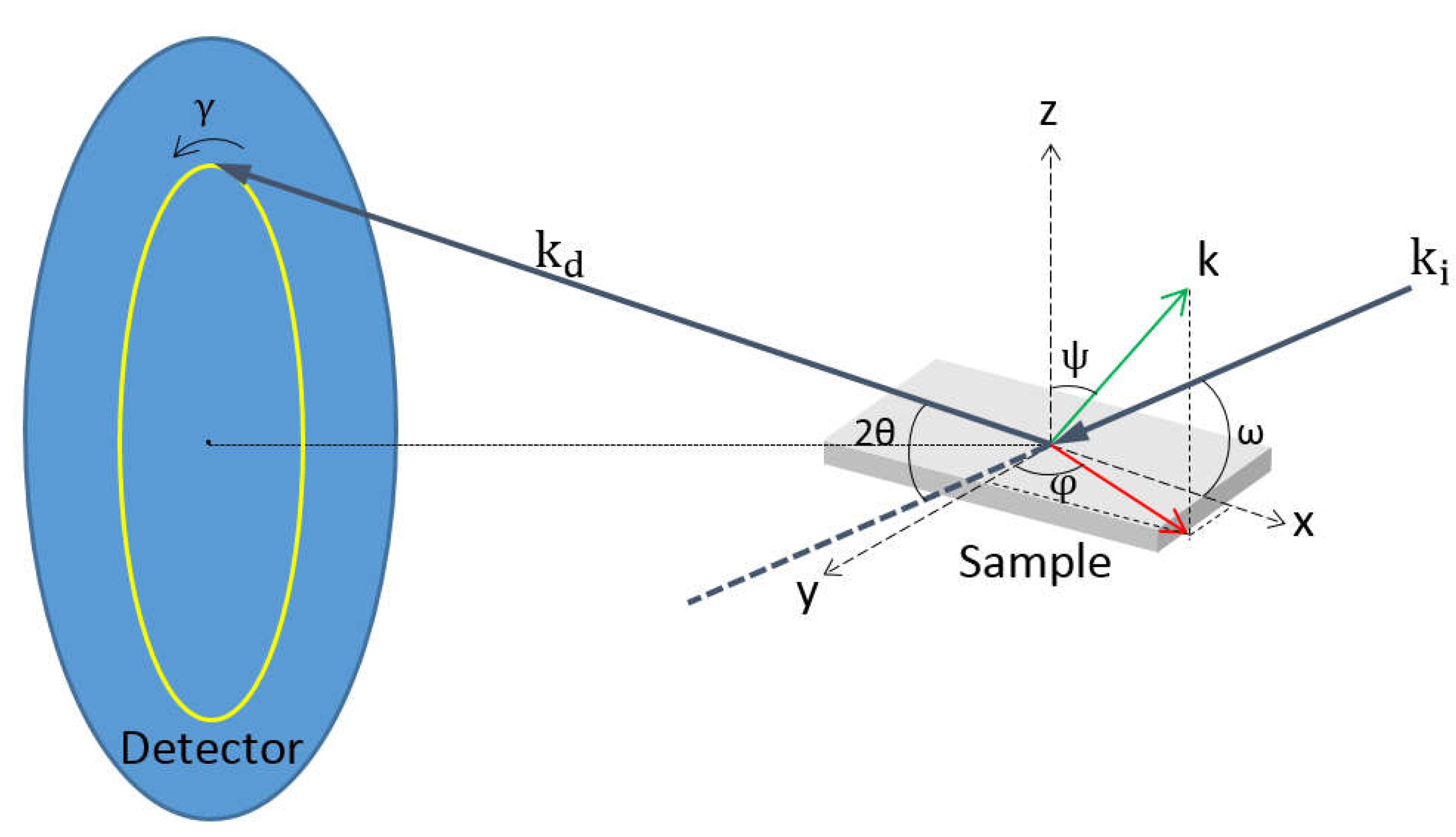
2.2.1. Experimental Setup
- Note the detected intensity of the uncut incident beam
- Adjust the sample to partially cut off the incident beam, detected intensity is then less than the previous intensity
- Rotate the sample around the axis to find the ideal position, for which the detected intensity is maximum. After this adjustment, the surface of the sample is then parallel to the incident beam
- Adjust precisely the height of the sample so that the detected intensity is equal to the ideal position
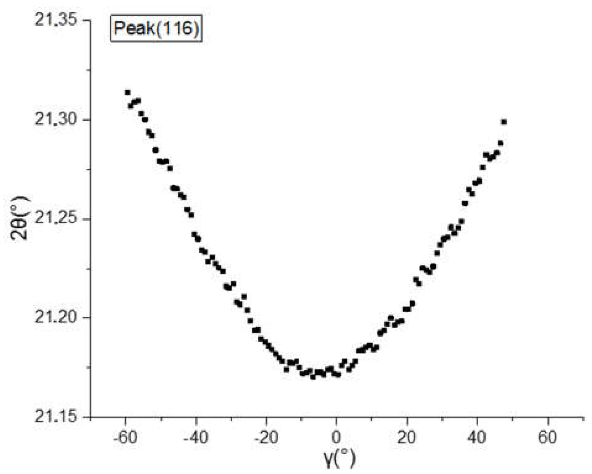
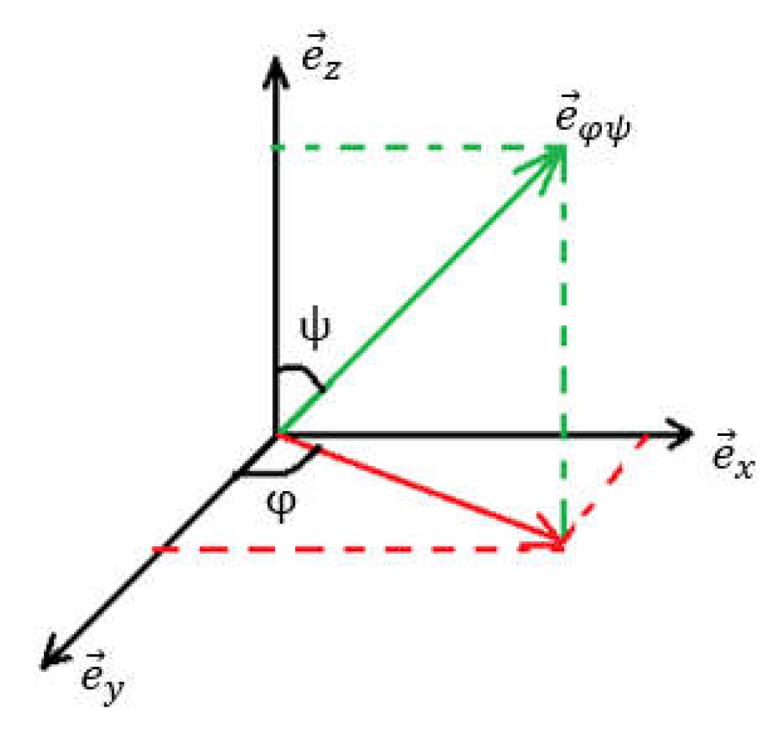
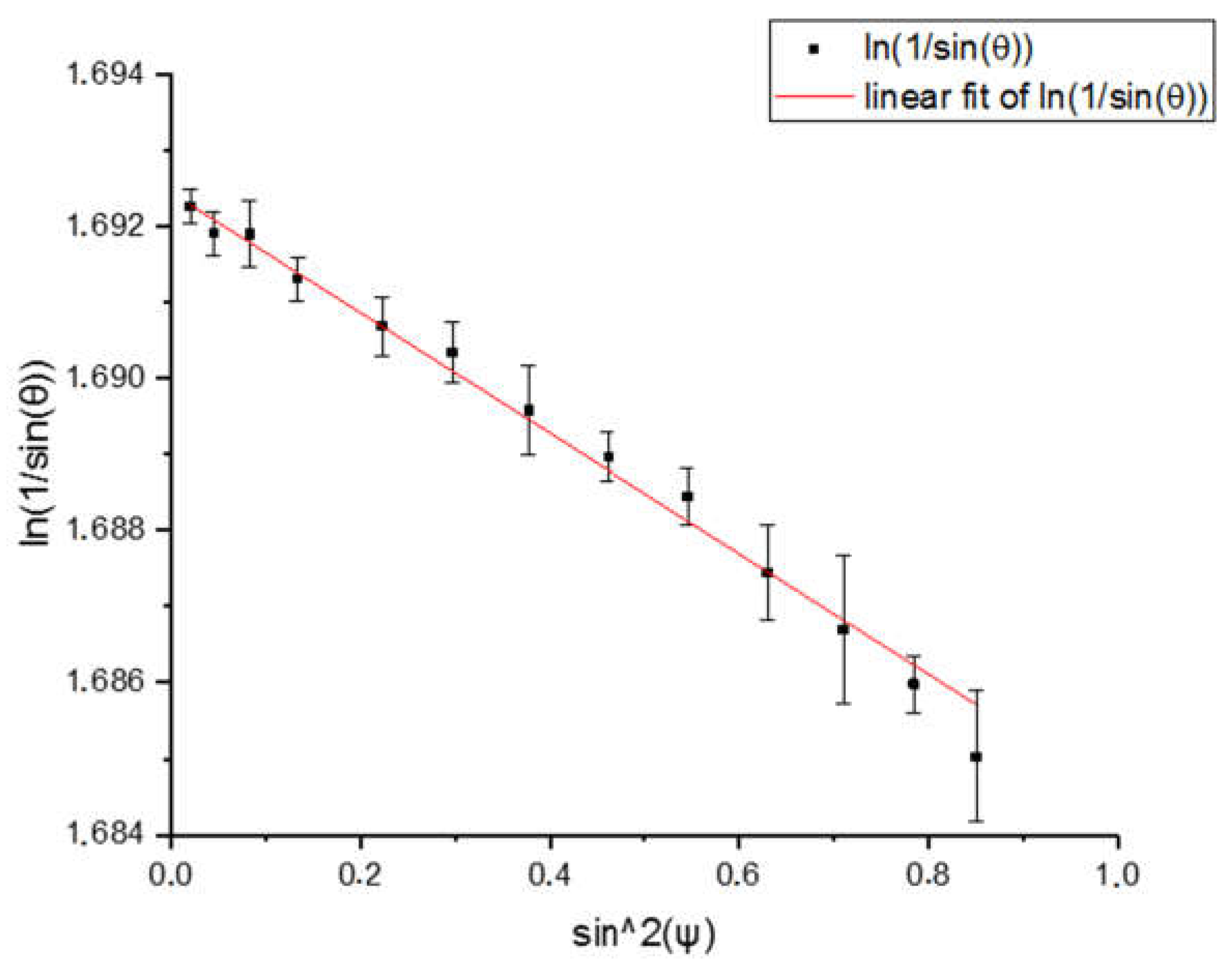
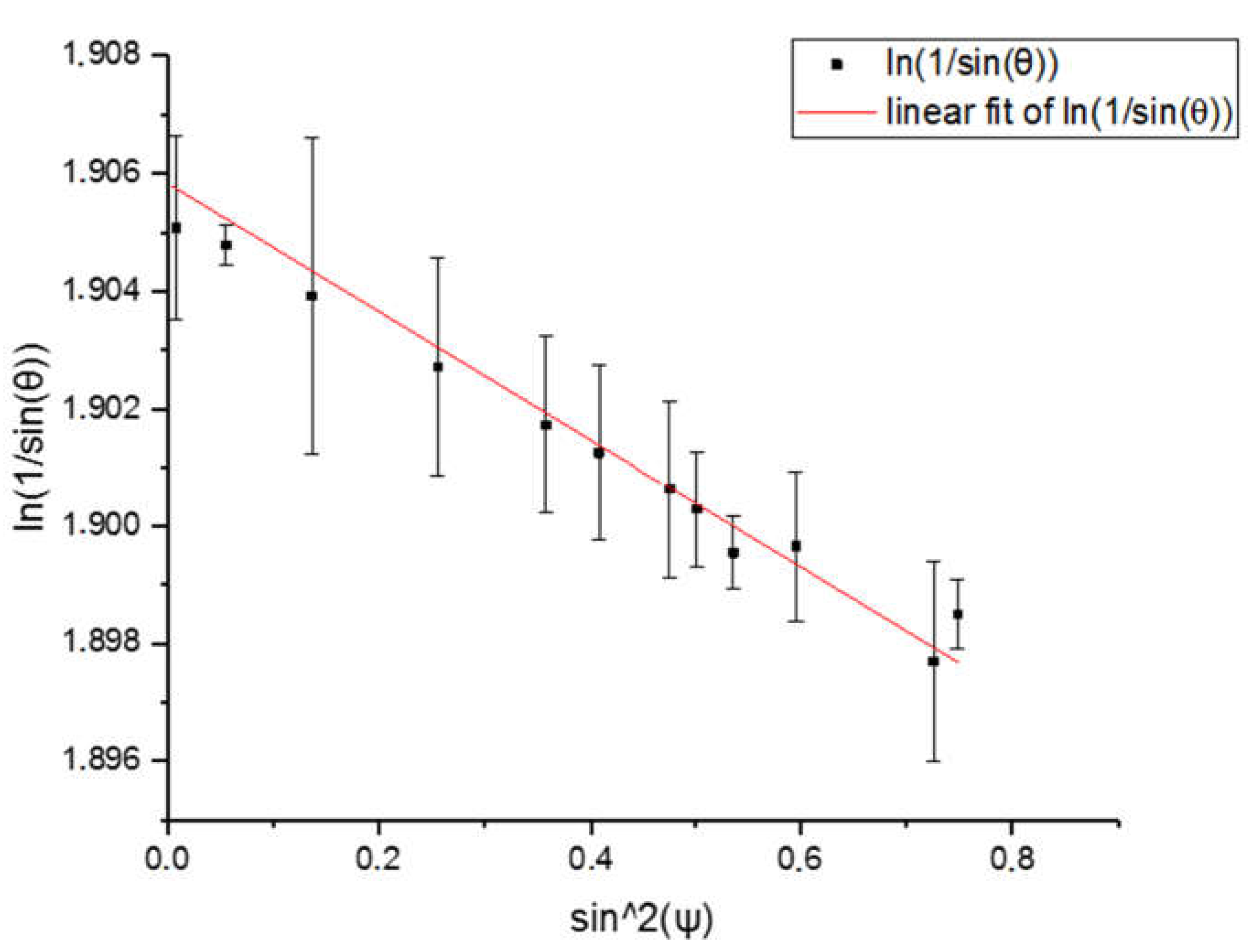
2.2.2. Sin2ψ Method
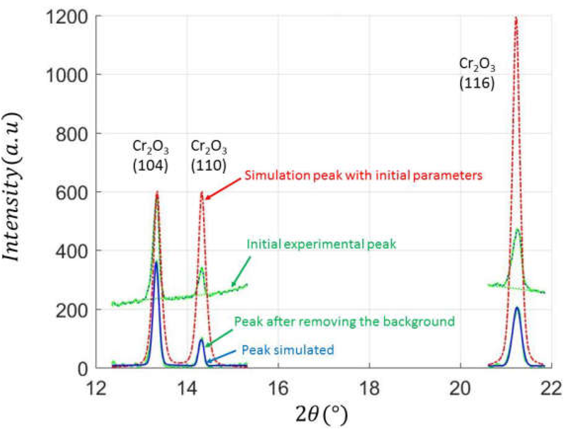
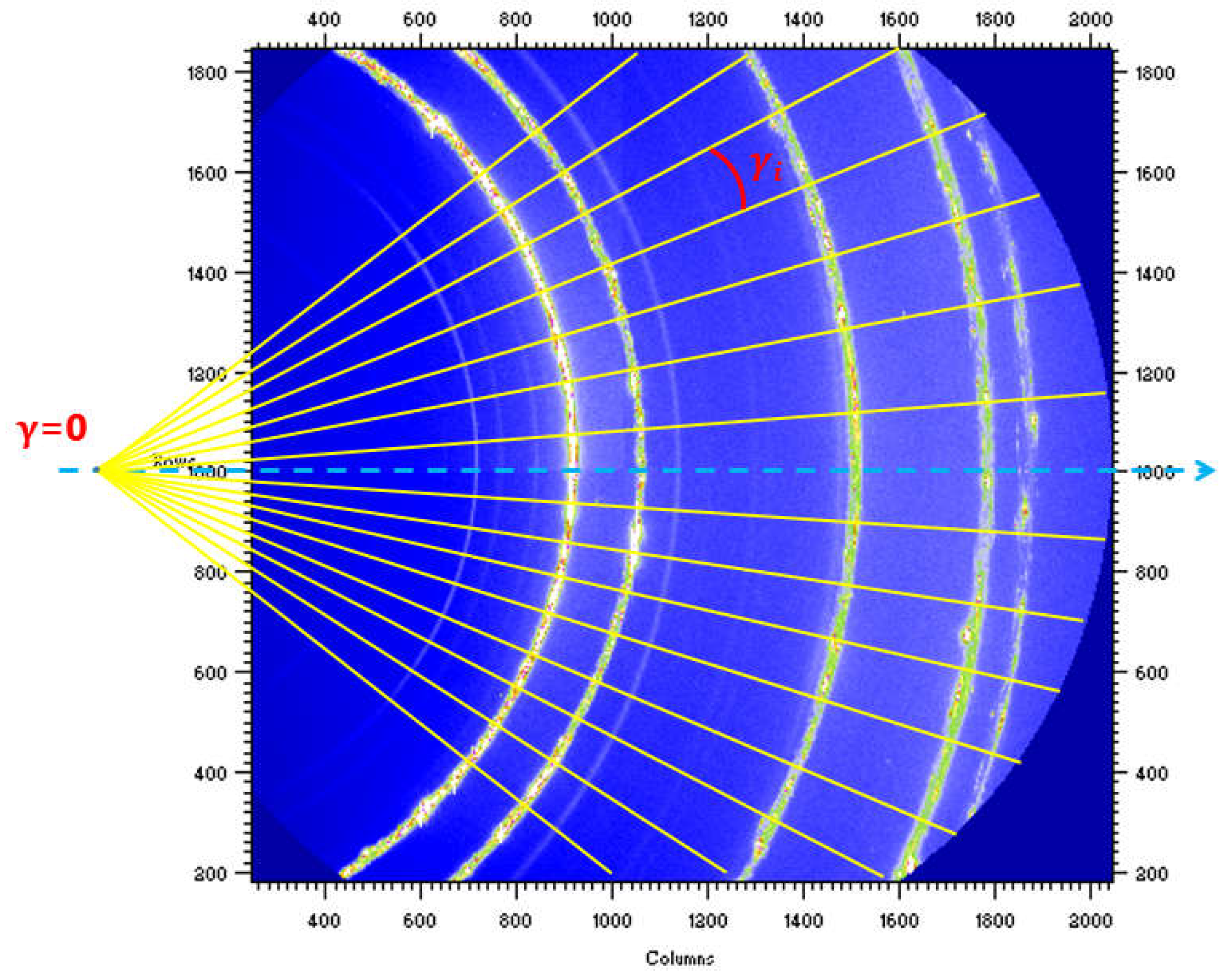
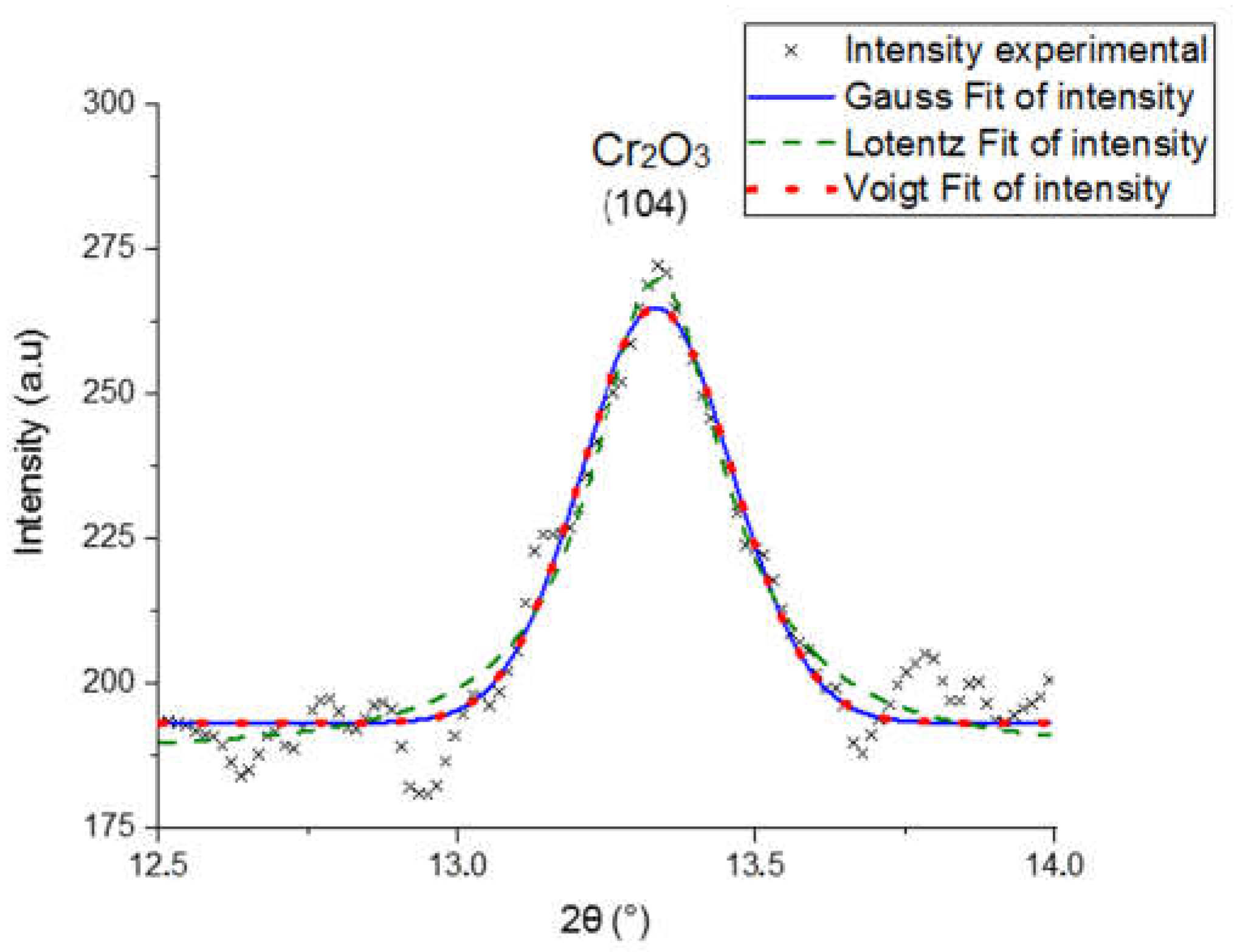
2.2.3. Data Processing
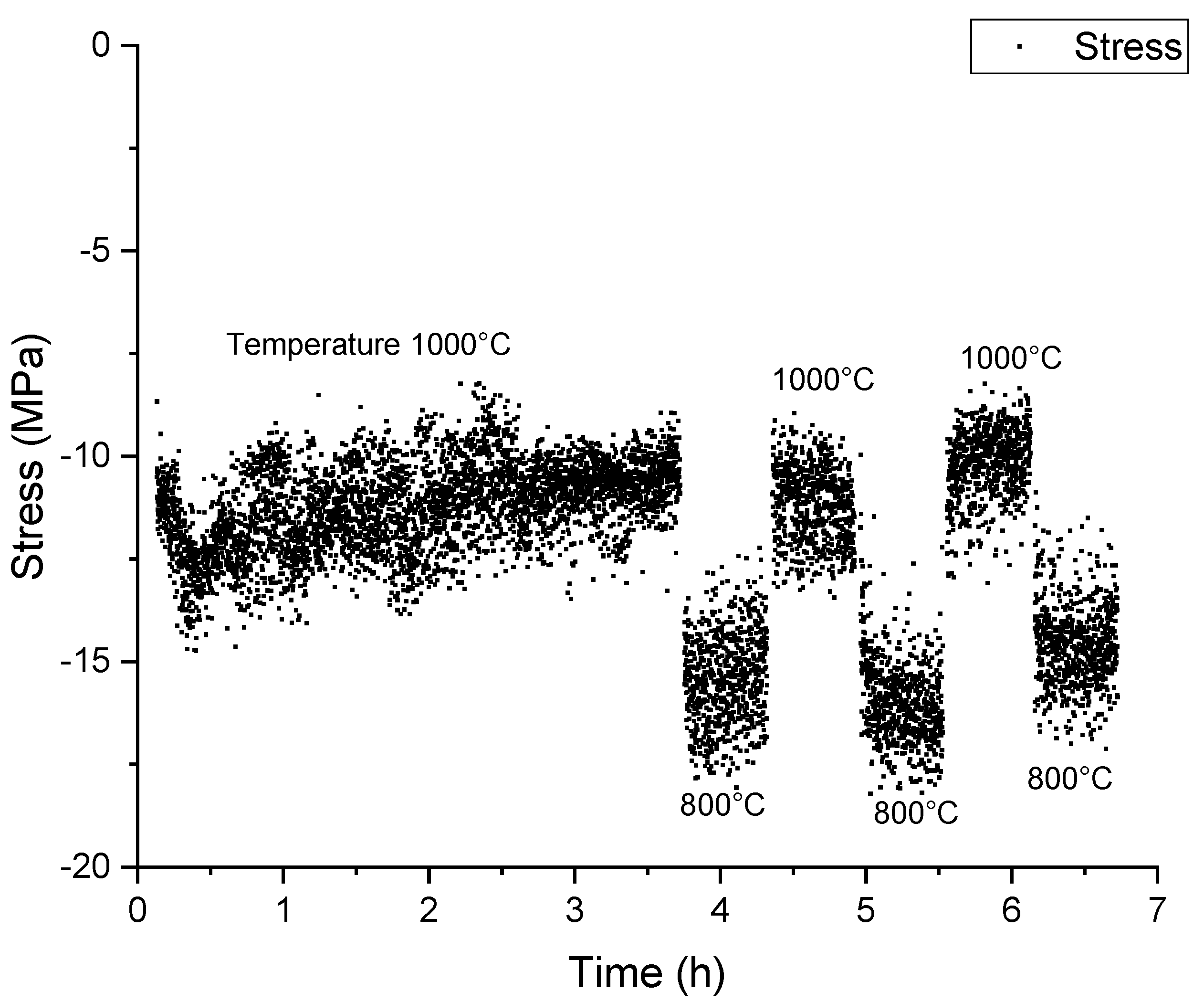
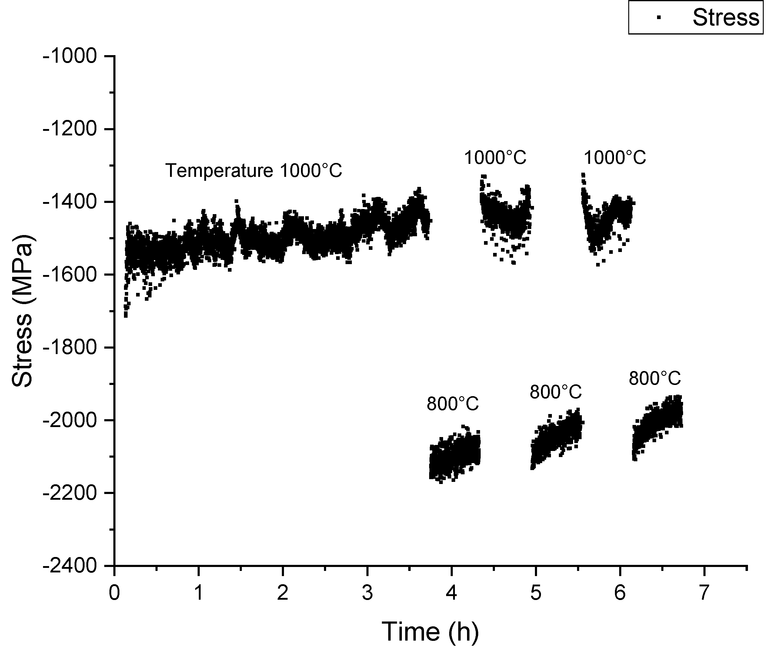
2.2.4. Stress versus Time Results
2.3. Stress Corrections
- Dilatation correction: at the beginning of each temperature plateau, a procedure is applied to adjust the position of the sample; its height is corrected from the dilation effect. Therefore, the X-ray should irradiate the same place, whatever the temperature is. However, an uncertainty is associated to this correction step.
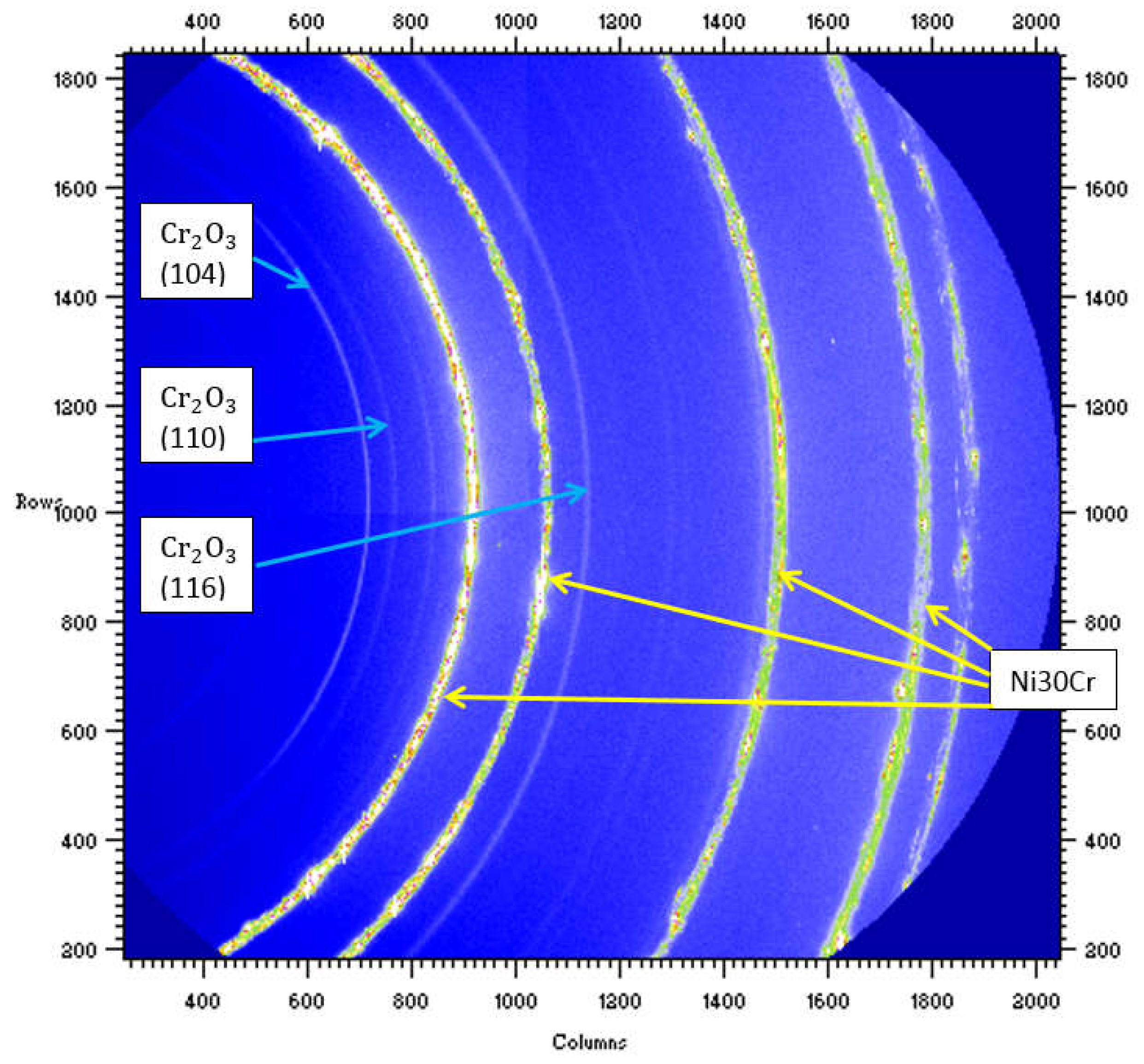
- Calibration procedure: to get the angular positions of the diffracted rings, it is necessary to establish a correspondence between the rings and pixels positions on the area images. To achieve such a goal, the obtained raw data have been systematically corrected by using references standard positions (NIST Silicon or Cr2O3) analyzed in the same diffraction conditions. However, an uncertainty is also associated to this procedure.
2.3.1. Correction with Method 1
2.3.2. Correction with Method 2
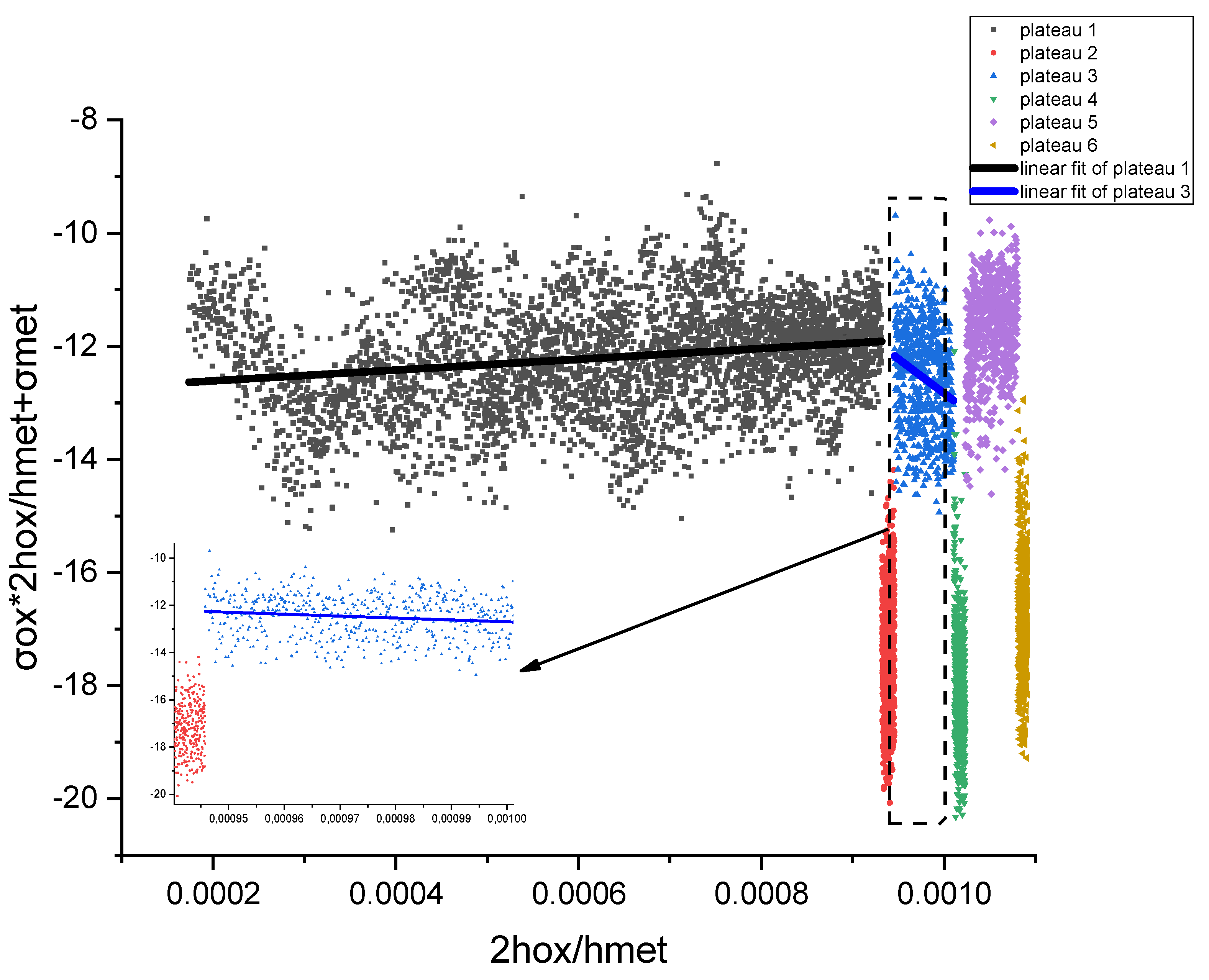
2.3.3. Offset Calculation
3. Results
3.1. Stress Evoution in the Metal Taking into Account the Offset Correction
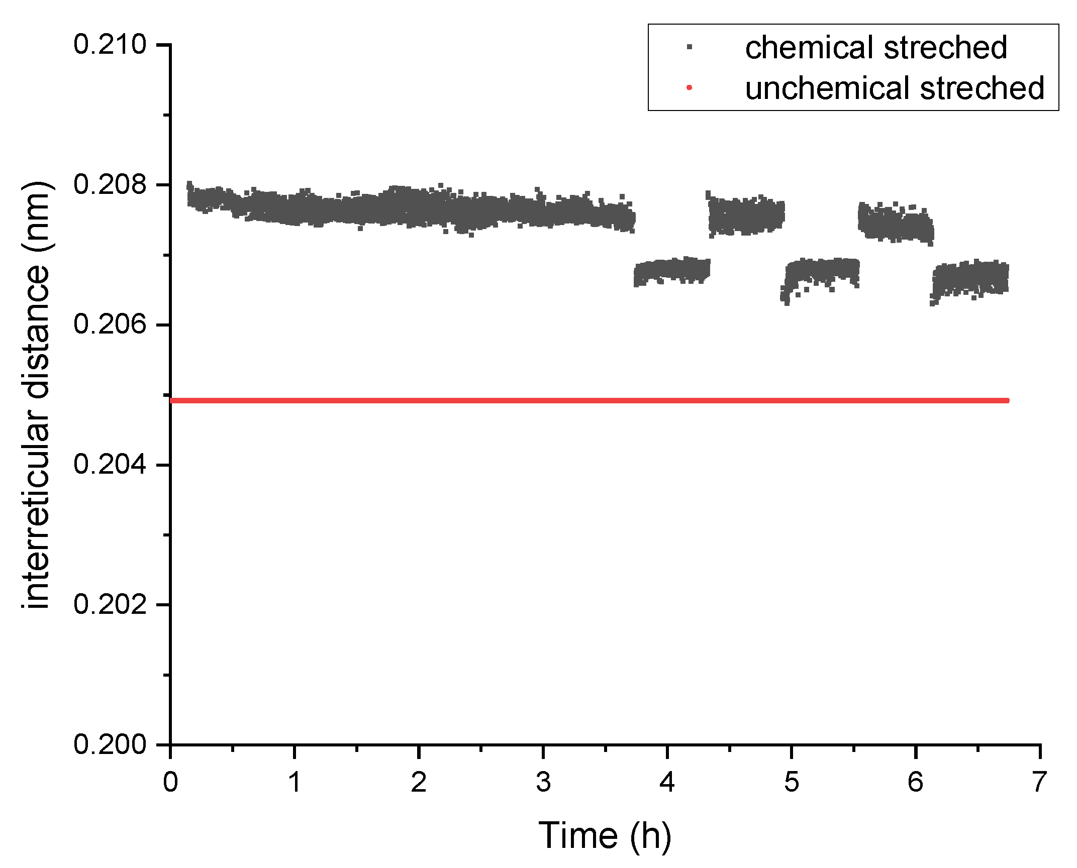
3.2. Influence of the Experimental and Physical Parameters on the Interreticular Distance
4. Conclusions
Author Contributions
Funding
Acknowledgments
Conflicts of Interest
References
- Schütze, M. Protective Oxide Scales and Their Breakdown; Wiley: Hoboken, NJ, USA, 1991. [Google Scholar]
- Kofstadt, P. High Temperature Corrosion; Elsevier: London, UK, 1998. [Google Scholar]
- Huntz, A.M.; Pieraggi, B. Oxydation des Matériaux Métalliques; Hermès Science: Paris, France, 2003. [Google Scholar]
- Panicaud, B.; Grosseau-Poussard, J.L.; Tao, Z.; Rakotovao, F.; Geandier, G.; Renault, P.O.; Goudeau, P.; Boudet, N.; Blanc, N. Frequency analysis for investigation of the thermomechanical mechanisms in thermal oxides growing on metals. Acta Mech. 2017, 228, 3595–3617. [Google Scholar] [CrossRef]
- Panicaud, B.; Grosseau-Poussard, J.L.; Kemdehoundja, M.; Dinhut, J.F. Mechanical features optimization for α-Cr2O3 oxide films growing on alloy NiCr30. Comput. Mater. Sci. 2009, 46, 42–48. [Google Scholar] [CrossRef]
- Tao, Z.J.; Rakotovao, F.; Grosseau-Poussard, J.L.; Panicaud, B. Determination of stress fields and identification of thermomechanical parameters in a thermally grown oxide under thermal cycling loadings, using advanced models. Adv. Mater. Res. 2014, 996, 896–901. [Google Scholar] [CrossRef]
- Ruan, J.L.; Pei, Y.; Fang, D. Residual stress analysis in the oxide scale/metal substrate system due to oxidation growth strain and creep deformation. Acta Mech. 2012, 223, 2597–2607. [Google Scholar] [CrossRef]
- Faurie, D.; Geandier, G.; Renault, P.-O.; Le Bourhis, E.; Thiaudière, D. Sin2ψ analysis in thin films using area detectors: non-linearity due to set-up, stress state and microstructure. Thin Solid Films 2013, 530, 25–29. [Google Scholar] [CrossRef]
- François, M. Unified description for the geometry of X-ray stress analysis: proposal for a consistent approach. J. Appl. Crystallogr. 2008, 41, 44–55. [Google Scholar] [CrossRef]
- Liu, J.; Saw, R.E.; Kiang, Y.-H. Calculation of Effective Penetration Depth in X-ray Diffraction for Pharmaceutical Solids. J. Pharm. Sci. 2010, 99, 3807–3814. [Google Scholar] [CrossRef] [PubMed]
- Faraoun, H.; Aourag, H.; Esling, C.; Seichepine, J.L.; Coddet, C. Elastic properties of binary NiAl, NiCr and AlCr and ternary Ni2AlCr alloys from molecular dynamic and Abinitio simulation. Comput. Mater. Sci. 2005, 33, 184–191. [Google Scholar] [CrossRef]
- Abdullah, M.M.; Rajab, F.M.; Al-Abbas, S.M. Structural and optical characterization of Cr2O3 nanostructures: Evaluation of its dielectric properties. AIP Adv. 2014, 4, 027121. [Google Scholar] [CrossRef]
- Ionescu, C.C. Caractérisation des mécanismes d’usure par tribocorrosion d’alliages modèles Ni–Cr. Ph.D. Thesis, École Centrale Paris, Paris, France, 2012. [Google Scholar]
- Trindade, V.B.; Krupp, U.; Hanjari, B.Z.; Yang, S.; Christ, H.-J. Effect of alloy grain size on the high-temperature oxidation behavior of the austenitic steel TP 347. Mater. Res. 2005, 8, 371–375. [Google Scholar] [CrossRef]
- Rakotovao, F.N. Relaxation des contraintes dans les couches de chromine développées sur alliages modèles (NiCr et Fe47Cr): Apport de la diffraction in-situ à haute température sur rayonnement Synchrotron à l’étude du comportement viscoplastique: effets d’éléments réactifs. Ph.D. Thesis, Université de La Rochelle, La Rochelle, France, 2016. [Google Scholar]
- Tao, Z.J. Etude expérimentale et modélisation des caractéristiques mécaniques d’une couche d'oxyde sous charges thermiques. Ph.D. Thesis, Université de Technologie de Troyes, Troyes, France, 2018. [Google Scholar]
- Guerain, M. Contribution à l'étude des mécanismes de relaxation de contraintes dans les films de chromine sur Ni-30Cr et Fe-47Cr: approche multi-échelles par spectroscopie Raman et microdiffraction Synchrotron. Ph.D. Thesis, Université de La Rochelle, La Rochelle, France, 2012. [Google Scholar]
- JCPDS DATABASE; Provided with Bruker Diffractometer; Bruker: Billerica, MA, USA, 2017.
- Petrović, S.; Bundaleski, N. Structure and surface composition of NiCr sputtered thin films. Sci. Sinter. 2006, 38, 155–160. [Google Scholar] [CrossRef]


| Ni. | Cr | Si | Mn | C (ppm) | P (ppm) | S (ppm) |
|---|---|---|---|---|---|---|
| 69.65 | 30.22 | <0.01 | <0.01 | 230 | 30 | 40 |
| 800 °C | ||||
| Stiffness | Cr2O3 (104) | Cr2O3 (110) | Cr2O3 (116) | Ni30Cr (111) |
| (TPa−1) | −0.824 | −1.018 | −0.805 | −1.622 |
| 0.5 (TPa−1) | 3.987 | 4.557 | 3.927 | 6.886 |
| 1000 °C | ||||
| Stiffness | Cr2O3 (104) | Cr2O3 (110) | Cr2O3 (116) | Ni30Cr (111) |
| (TPa−1) | −0.817 | −1.010 | −0.867 | −1.837 |
| 0.5 (TPa−1) | 3.999 | 4.561 | 4.136 | 7.752 |
| Plane (hkl) Cr2O3 | (104) | (110) | (116) | Plane (hkl) | NiCr (111) |
|---|---|---|---|---|---|
| 2θ Theoretical (°) | 13.25 | 14.30 | 21.20 | 2θ Theoretical (°) | 17.22 |
| Phase | Variation of | Minimum Error Bar | Maximum Error Bar | Average Error Bar | Proportion of Average Error Bar |
|---|---|---|---|---|---|
| Oxide | 7.2 × 10⁻³ | 2.3 × 10⁻⁴ | 9.8 × 10⁻⁴ | 4.8 × 10⁻⁴ | 6.7% |
| Metal | 7.4 × 10⁻³ | 3.5 × 10⁻⁴ | 2.7 × 10⁻³ | 1.3 × 10⁻³ | 17.6% |
| Temperature (°C) | 800 | 900 | 1000 |
|---|---|---|---|
| ( ) | 2.18 × 10⁻¹³ | 6.08 × 10⁻¹³ | 5.56 × 10⁻¹² |
| Plan (hkl) Cr2O3 | (104) | (110) | (116) | Plan (hkl) NiCr | (111) |
|---|---|---|---|---|---|
| Distances between crystallographic planes (nm) | 0.2665 | 0.24794 | 0.16725 | Distances between crystallographic planes (nm) | 0.20492 |
© 2018 by the authors. Licensee MDPI, Basel, Switzerland. This article is an open access article distributed under the terms and conditions of the Creative Commons Attribution (CC BY) license (http://creativecommons.org/licenses/by/4.0/).
Share and Cite
Wang, Z.; Grosseau-Poussard, J.-L.; Panicaud, B.; Geandier, G.; Renault, P.-O.; Goudeau, P.; Boudet, N.; Blanc, N.; Rakotovao, F.; Tao, Z. Determination of Residual Stresses in an Oxidized Metallic Alloy under Thermal Loadings. Metals 2018, 8, 913. https://doi.org/10.3390/met8110913
Wang Z, Grosseau-Poussard J-L, Panicaud B, Geandier G, Renault P-O, Goudeau P, Boudet N, Blanc N, Rakotovao F, Tao Z. Determination of Residual Stresses in an Oxidized Metallic Alloy under Thermal Loadings. Metals. 2018; 8(11):913. https://doi.org/10.3390/met8110913
Chicago/Turabian StyleWang, Zhimao, Jean-Luc Grosseau-Poussard, Benoît Panicaud, Guillaume Geandier, Pierre-Olivier Renault, Philippe Goudeau, Nathalie Boudet, Nils Blanc, Felaniaina Rakotovao, and Zhaojun Tao. 2018. "Determination of Residual Stresses in an Oxidized Metallic Alloy under Thermal Loadings" Metals 8, no. 11: 913. https://doi.org/10.3390/met8110913
APA StyleWang, Z., Grosseau-Poussard, J.-L., Panicaud, B., Geandier, G., Renault, P.-O., Goudeau, P., Boudet, N., Blanc, N., Rakotovao, F., & Tao, Z. (2018). Determination of Residual Stresses in an Oxidized Metallic Alloy under Thermal Loadings. Metals, 8(11), 913. https://doi.org/10.3390/met8110913