Mathematical Model for Prediction and Optimization of Weld Bead Geometry in All-Position Automatic Welding of Pipes

Abstract

In this study all-position automatic tungsten inert gas (TIG) welding was exploited to enhance quality and efficiency in the welding of copper-nickel alloy pipes. The mathematical models of all-position automatic TIG weld bead shapes were conducted by the response surface method (RSM) on the foundation of central composition design (CCD). The statistical models were verified for their significance and adequacy by analysis of variance (ANOVA). In addition, the influences of welding peak current, welding velocity, welding duty ratio, and welding position on weld bead geometry were investigated. Finally, optimal welding parameters at the welding positions of 0° to 180° were determined by using RSM.

1. Introduction

With the fast development of heavy industries, all-position automatic tungsten inert gas (TIG) welding of pipes had been widely applied to industries such as shipbuilding, nuclear power, chemical industries, and natural gas transportation. Welding plays an important role in joining pipes [1]. Traditional all-position welding of pipes is manual arc welding, but it has low welding efficiency, poor stability, and high cost. Moreover, the manual operation of pipe welding is a challenge to the welder. In order to overcome the aforementioned shortcomings of manual arc welding, an all-position automatic TIG welding process has been developed in recent years. At present, there are four types of automatic TIG butt-welding equipment for pipelines: closed welding heads, open welding heads, orbital welding trolleys, and thick-walled narrow gap TIG welding heads.

In all-position automatic TIG welding of pipes, especially for vertical and overhead position welding, it is a challenge to control the liquid metal flow down from the molten pool under the action of gravity. Therefore, there is a need to adjust welding parameters to keep the droplet transition smooth. In order to obtain high-quality weld beads, selecting optimal weld parameters and controlling the weld bead profile are important. As is well known, weld bead shape has a noteworthy influence on the mechanical properties of lap joints. In all-position automatic TIG welding of pipes, the weld bead profile is impacted not only by the weld parameters such as weld background current, weld peak current, weld speed, weld voltage, but also by the welding position. Therefore, it is hard to obtain several optimal parameters to receive perfect weld bead profiles. To realize this goal, the connection between weld parameters and weld bead shapes need to be established. A lot of research has been undertaken to establish mathematical models to optimize parameters and obtain the relationship [2,3]. Xu et al. [4] optimized the narrow gap all-position gas metal arc (GMA) welding parameters by employing the response surface method (RSM) and building regression models to predict the parameters of weld bead geometry. Rao et al. [5] had obtained the influence of welding parameters and statistical models for the prediction of weld bead shapes in pulsed GMA welding. Koleva [6] researched the connection with electron beam welding parameters and weld bead geometry; moreover, the mathematical model can optimize welding parameters. Karthikeyan and Balasubramanian used RSM to optimize friction stir spot welding procedure parameters and to obtain maximum lap shear strength of the lap joint [7]. The statistical model was built at an invariable position in inchoate research. However, in all-position automatic TIG welding of pipes, the welding position should be used as the input parameter of the statistical model because the weld includes flat, vertical and overhead positions [8], and welding position impacts the weld bead profile.

RSM can be used to predict the weld bead shape and mechanical properties in the welding process [9,10,11,12]. The ultimate goal of this paper is to build a new all-position automatic TIG pipes’ welding procedure and a mathematical model of weld bead geometry using RSM.

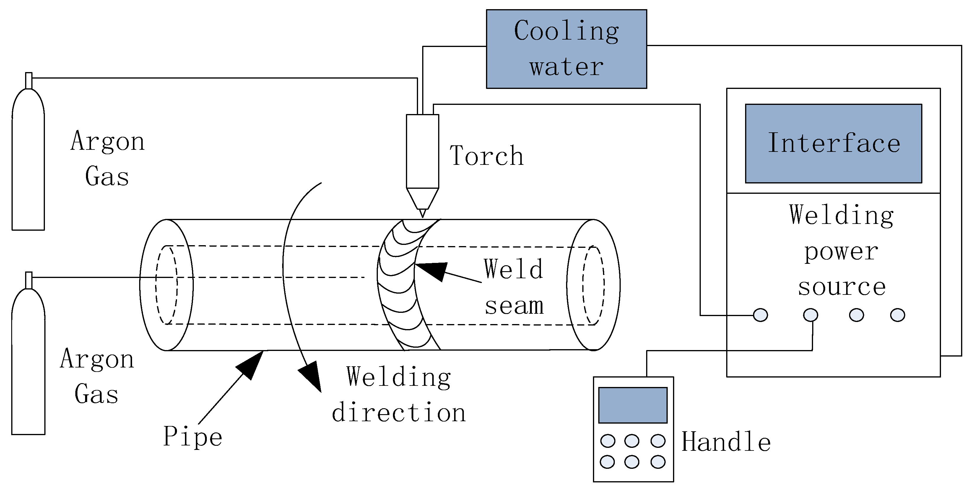
2. Materials and Methods

The schematic diagram of the system for all-position automatic TIG welding of pipelines is shown in Figure 1. The system includes an iOrbital 5000 welding machine, a TOA77 welding torch, a control panel, two argon tanks, a welding fixture and a cool water circulation system. The welding process was as follows:

Figure 1. The schematic diagram of the system for all-position automatic tungsten inert gas (TIG) welding of pipes.

(1)

Fixing the pipes with a welding fixture.

(2)

Inputting the cool water and argon gas into the TOA77 welding torch.

(3)

The protective gas was inputted into the pipes.

(4)

The welding torch weld around the pipes.

The workpieces used in this study are UNS (Unified Numbering System for Metas and Alloys) C70600 with dimensions of Φ57 mm × 300 mm × 2 mm, but there is a flaring end of the pipe and the diameter is 62 mm, as shown in Figure 2. The chemical compositions of the parent metal are listed in Table 1. In this study, experiments were executed with one-sided welding with double-sided shaping without an opening groove and welding wire, because the experiments melt the parent metal as filler metals. There is an angle of 30 degrees between the torch and the pipe vertical direction. Before welding, two pipes without a groove were fixed with a gap of 0.5 mm, and they were then lap welded. To ensure the stability of the welding process and avoid weld joints from being influenced by impurities and surface oil contamination, the pipes should be cleaned before welding. Pure argon (99.9% purity) was selected as a shielding gas with a flow rate of 15 L/min on the surface of the pipes and a flow rate of 20 L/min in the pipes to prevent the base metal from oxidizing in the air and enhancing the quality of the weld bead. The tungsten electrode diameter was 3.2 mm and the taper was 60°.

Figure 2. The schematic diagram of the lap joint.

Table 1. Chemical compositions of parent metal (wt%).

Chemical Element	Ni	Fe	Mn	Pb	S	C	Zn	P	Cu
Measured Value	10.66	1.60	0.79	0.01	0.0023	0.0065	0.019	0.01	Bal

In Figure 3, the specimens for weld bead shape observation were cut from the cross-section of the pipes, sealed with bake lite resin, then ground with a series of emery papers (grit size 400, 600, 800, 1200, 1500, 2000 and 2500), polished with a 1.0-μm diamond paste, and etched with an etchant of 5 g ferric chloride + 16 mL hydrochloric acid + 60 mL ethanol. Finally, a high-dynamic camera model NSC1003 (New Imaging Technologies, Paris, France) was used to photograph the weld bead shape and calculate the weld width, weld depth and weld thickness by image processing software. Reducing measurement error is important to the experiments, and therefore each value was measured three times. Then the average of the three measured values was calculated as experimental data.

Figure 3. The cross-section of the weld bead. (weld width (W), weld depth (D), weld thickness (T)).

In this investigation, due to the working range of individual factor being extensive, a central composition rotatable four-factor, five-level factorial design matrix was selected. The design software Design-Expert (V 10. 0. 7, Stat-Ease, MN, USA) was used to establish the design matrix and process the experimental data.

The steps of this investigation are as follows:

(a)

Validation of the primary factors;

(b)

Confirming the working range of the control variables;

(c)

Establishing trial matrix by Design-Expert V10.0.7 software;

(d)

Conducting the experiments as per the design matrix;

(e)

Recording the response parameters;

(f)

Building statistical models;

(g)

Calculating regression coefficients of the multinomial;

(h)

Checking the adequacy of the statistical model;

(i)

Verification of models;

(j)

Receiving, finally, the statistical model;

(k)

Analysis of results;

(l)

Optimizing welding parameters.

3. Creating Mathematical Model

Based on the initial experimental results, four very important welding parameters affecting the weld bead geometry are the welding peak current (I), welding velocity (V), welding duty ratio (d) and welding position (P). The duty ratio is the ratio of welding peak current time to the pulse period. In order to create a mathematical model to describe and forecast the weld bead geometry in all-position automatic welding, I, V, d, and P were chosen as input parameters. The schematic diagrams of the weld bead shape and welding position are shown in Figure 3 and Figure 4, respectively.

Figure 4. Schematic diagram of welding position.

Before this experiment, the control variable method was used to find out the working range of input parameters. The working range was determined by the steady welding procedure and invisible weld defects. In order to obtain optimized welding parameters, the establishment of a test parameter matrix adopts the center composed design (CCD) in the regression design method. In the CCD design, the upper and lower limit values of the input parameters were coded as ± β, the value of β is dependent on the number of input parameters and β = ${(2^k)}^{1/4}$, k is the number of input parameters. The upper level and lower level were coded as ±1 respectively and the center point was coded as 0. In this research, there are 4 input parameters, so β is 2. Therefore, the upper and lower limit values of the input parameters were coded as ±2. The codes values for intermediate levels can be calculated by Equation (1):

$$X_i=2\left[2X-\left(X_{max}+X_{min}\right)\right]/\left[X_{max}-X_{min}\right]$$

(1)

In Equation (1), $X_i$ is the desired code value of a variable $X$, and range of values of $X$ is from $X_{min}$ to $X_{max}$; $X_{max}$ is the upper limits and $X_{min}$ is lower limits of the variable $X$ [13,14].

The factor levels and coded values have been listed in Table 2. The experimental design matrix (Table 3) includes 30 sets of coded situations and constitutes a full replication four-factor factorial design of 16 points, 8 star points and 6 center points [7].

Table 2. Important weld parameters and their levels for copper–nickel alloy pipe.

Factors	Unit	Coded Value
		−2	−1	0	1	2
I	A	114	117	120	123	126
V	mm/min	57	60	63	66	69
d	%	40	45	50	55	60
P	°	0	45	90	135	180

Table 3. Trial design matrix and response of copper–nickel alloy lap joints.

Std	Run	Coded Variables				Response Parameters
		I (A)	V (mm/min)	D (%)	P (degree)	W (mm)	D (mm)	T (mm)
1	7	117	60	45	45	1.416	0.29	1.978
2	10	123	60	45	45	1.615	0.363	2.142
3	6	117	66	45	45	1.016	0.199	1.797
4	19	123	66	45	45	1.325	0.272	1.89
5	11	117	60	55	45	2.877	0.577	2.541
6	24	123	60	55	45	4.2	0.851	2.751
7	22	117	66	55	45	1.575	0.315	1.995
8	26	123	66	55	45	2.373	0.462	2.232
9	29	117	60	45	135	3.255	0.637	2.185
10	30	123	60	45	135	4.956	1.02	2.314
11	14	117	66	45	135	2.583	0.525	1.932
12	8	123	66	45	135	3.591	0.706	2.73
13	5	117	60	55	135	4.074	0.835	3.024
14	23	123	60	55	135	5.796	1.298	2.541
15	16	117	66	55	135	3.297	0.606	2.379
16	15	123	66	55	135	5.754	1.179	2.034
17	12	114	63	50	90	2.268	0.441	2.331
18	28	126	63	50	90	3.717	0.762	2.436
19	20	120	57	50	90	3.402	0.697	2.667
20	9	120	69	50	90	2.856	0.462	1.827
21	27	120	63	40	90	2.226	0.356	1.659
22	4	120	63	60	90	5.859	1.201	2.478
23	13	120	63	50	0	0.987	0.202	1.533
24	17	120	63	50	180	4.032	0.826	2.184
25	3	120	63	50	90	3.412	0.699	2.331
26	2	120	63	50	90	3.533	0.724	2.826
27	25	120	63	50	90	3.641	0.528	2.461
28	21	120	63	50	90	2.755	0.597	2.098
29	1	120	63	50	90	2.562	0.74	2.356
30	18	120	63	50	90	2.878	0.742	2.501

In order to better reflect the weld bead geometry, reasonable response parameters need to be selected. The response parameters were named weld width (W), weld depth (D), and weld thickness (T). Figure 3 shows the cross section of weld bead.

On the foundation of central composite design matrix, the value of input parameters, response parameters and the regression model can be built. The connection between measured response and the input parameters could be shown as y = f ($x_1$, $x_2$,…, $x_i$) + ε, where y is the value of measured response, $x_i$ is the value of the input parameter, and ε is the systematic error. Y is a power transformation of y [11,15], so the second-order polynomial can be expressed as Equation (2):

$$Y=b_0+{\sum }_{i=1}^4{b}_i{x}_i+{\sum }_{i=1}^3{\sum }_{j=i+1}^4{b}_{ij}{x}_i{y}_j+{\sum }_{i=1}^4{b}_{ii}{x}_i{}^2$$

(2)

where, b₀ is the average of the measured response, the regression coefficients such as b_i, b_ij and b_ii depend on linear, interaction and squared terms of factors, respectively.

Almost all response surface method problems can be approximated by these polynomials, and the regression coefficients could be obtained by the least squares method.

The regression model adopts the method of stepwise regression. Firstly, the regression model eliminates the insignificant terms and calculates the regression coefficients until the significant terms and the lack-of-fit terms of the regression model meet the requirements of the regression model. Finally, the relational expressions about all-position automatic TIG welding of the pipe within the range of 0–180° were obtained as Equations (3)–(8), which show the relationship between weld geometry shape and input parameters.

The final equations in terms of coded factors are given as follows:

W = 3.07 + 0.52 I − 0.32 V + 0.73 d + 0.96 P + 0.19 I × d + 0.27 I × P + 0.22 d² − 0.16 P²

(3)

D = 0.64 + 0.12 I − 0.087 V + 0.16 d + 0.20 P + 0.047 I × d + 0.065 I × P + 0.034 d² − 0.032 P²

(4)

T = 2.36 + 0.042 I − 0.17 V + 0.17 d + 0.13 P − 0.098 I × d − 0.12 V × d − 0.11 P²

(5)

The final equations in terms of actual factors are given as follows:

W = 100.19346 − 0.64732 I − 0.10788 V − 2.29476 d − 0.20122 P + 0.012846 I × d + 0.00197176 I × P + 0.00898719 d² − 0.000783063 P²

(6)

D = 22.87088 − 0.15965 I − 0.028847 V − 0.47648 d − 0.050128 P + 0.00311250 I × d + 0.000478241 I × P + 0.00134656 d² − 0.0000160301 P²

(7)

T = −62.80003 + 0.34011 I + 0.34775 V + 1.32831 d + 0.012728 P − 0.00652083 I × d − 0.00811250 V × d − 0.0000546879 P²

(8)

Analysis of variance (ANOVA) was used to determine the significance and suitability of the regression model. Table 4, Table 5 and Table 6 show the ANOVA analysis of the weld width, the weld depth and the weld thickness model respectively.

Table 4. Results of analysis of variance (ANOVA) for model of weld width.

Source	Sum of Squares	df *	Mean Square	F Value	p Value (Prob > F)	Significance
Model	47.8	8	5.98	30.86	<0.0001	Significant
I	6.42	1	6.42	33.17	<0.0001	-
V	2.51	1	2.51	12.98	0.0017	-
d	12.69	1	12.69	65.56	<0.0001	-
P	22.04	1	22.04	113.82	<0.0001	-
I × d	0.59	1	0.59	3.07	0.0945	-
I × P	1.13	1	1.13	5.85	0.0247	-
d2	1.44	1	1.44	7.42	0.0127	-
P2	0.72	1	0.72	3.69	0.0683	-
Residual	4.07	21	0.19	-	-	-
Lack of Fit	3.04	16	0.19	0.92	0.5944	Not Significant
Pure Error	1.03	5	0.21	-	-	-
Cor total	51.87	29	-	-	-	-

* Degree of freedom (df), a concept in statics, indicates the number of unconstrained variables in calculating a statistical magnitude. According to the usual definition, df = n − k, n is the number of samples and k is the number of constrained variables or conditional number, while k is also the quantity of the other independent statistical magnitude in calculating one statistical magnitude.

Table 5. Results of ANOVA for model of weld depth.

Source	Sum of Squares	df	Mean Square	F Value	p Value (Prob > F)	Significance
Model	2.21	8	0.28	31.63	<0.0001	Significant
I	0.33	1	0.33	37.60	<0.0001	-
V	0.18	1	0.18	20.56	0.0002	-
d	0.6	1	0.6	68.85	<0.0001	-
P	0.93	1	0.93	106.39	<0.0001	-
I × d	0.035	1	0.035	3.99	0.0589	-
I × P	0.067	1	0.067	7.63	0.0117	-
d2	0.032	1	0.032	3.69	0.0685	-
P2	0.030	1	0.030	3.43	0.0782	-
Residual	0.18	21	0.008744	-	-	-
Lack of Fit	0.14	16	0.009019	1.15	0.4786	Not Significant
Pure Error	0.039	5	0.007863	-	-	-
Cor total	2.40	29	-	-	-	-

Table 6. Results of ANOVA for model of weld thickness.

Source	Sum of Squares	df	Mean Square	F Value	p Value (Prob > F)	Significance
Model	2.64	7	0.38	7.89	<0.0001	Significant
I	0.043	1	0.043	0.9	0.3544	-
V	0.72	1	0.72	15.15	0.0008	-
d	0.72	1	0.72	15.15	0.0008	-
P	0.40	1	0.40	8.46	0.0081	-
I × d	0.15	1	0.15	3.20	0.0872	-
V × d	0.24	1	0.24	4.96	0.0365	-
P2	0.35	1	0.35	7.39	0.0125	-
Residual	1.05	22	0.048	-	-	-
Lack of Fit	0.76	17	0.045	0.78	0.6845	Not Significant
Pure Error	0.29	5	0.058	-	-	-
Cor total	3.69	29	-	-	-	-

Using Design Expert V 10.0.7 Software can calculate the value of coefficient and the significance of each coefficient was confirmed by Student’s t test and p values. The values of “Prob > F” less than 0.0500 indicate model terms are significant and values greater than 0.1000 indicate the model terms are not significant [16,17]. Table 4, Table 5 and Table 6 show the result of ANOVA for the W model, D model and T models, respectively, and the models’ F values are 30.86, 31.63 and 7.89. The probability of F (prob > F) is less than 0.0001, in other words, these models are significant. Sometimes, these models show that the test results of lack-of-fit are insignificant relative to the pure error, insignificant lack-of-fit represents that the quadratic model is adequate. According to Table 4, I, d and P are the most important factors of the W model; V, (I × d), (I × P), d² and P² also could affect W. From Table 5, I, d and P are the most important factors of the D model; V, (I × d), (I × P), d² and P² also could affect D. I, V, d, P, (I × d), (V × d) and P² could affect T as shown in Table 6.

4. Verification of Models

To assure that the established model can predict and control the weld bead shape in actual application, it should test the accuracy of the mathematical model. The test experiments were executed by assigning diverse values for experimental variables within their working limits, but distinguishing them from the values of the design matrix. The values of input parameters, predicted response, actual response and percentage errors are listed in Table 7 respectively. It shows that the percentage errors for any models are less than 9%, and all the percentage errors are within the scope of industrial engineering requirements. Therefore, the statistical models can predict and optimize weld bead shape.

Table 7. Predicted values and actual values of the weld bead geometry.

Designation	Run	1	2	3	4	5
Input Parameters	I (A)	123	122	119	117	115
	V (mm/min)	60	60	60	62	63
	d (%)	55	45	40	60	55
	P (degree)	0	45	90	135	180
Predicted Values	W (mm)	1.977	1.818	2.788	3.958	4.067
	D (mm)	0.426	0.372	0.574	0.783	0.799
	T (mm)	2.071	2.091	2.194	2.707	2.406
Actual Values	W (mm)	1.839	1.978	2.581	3.615	4.256
	T (mm)	0.346	0.346	0.596	0.759	0.954
	W (mm)	2.204	1.991	2.345	2.891	2.278
Percentage Error ** (%)	W	−6.98	8.8	−7.43	−8.67	4.65
	D	−7.04	−6.99	3.38	−4.29	6.88
	T	6.42	−4.78	7.03	6.8	−5.32

** Percentage error = $\frac{actual value-predicted value}{predicted value}$ × 100.

5. Results and Discussion

According to the all models, the prime and interaction influences of input weld parameters on weld bead geometry can be found.

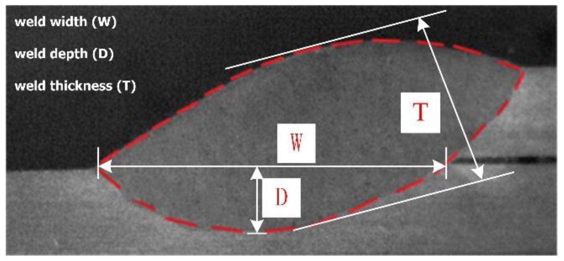
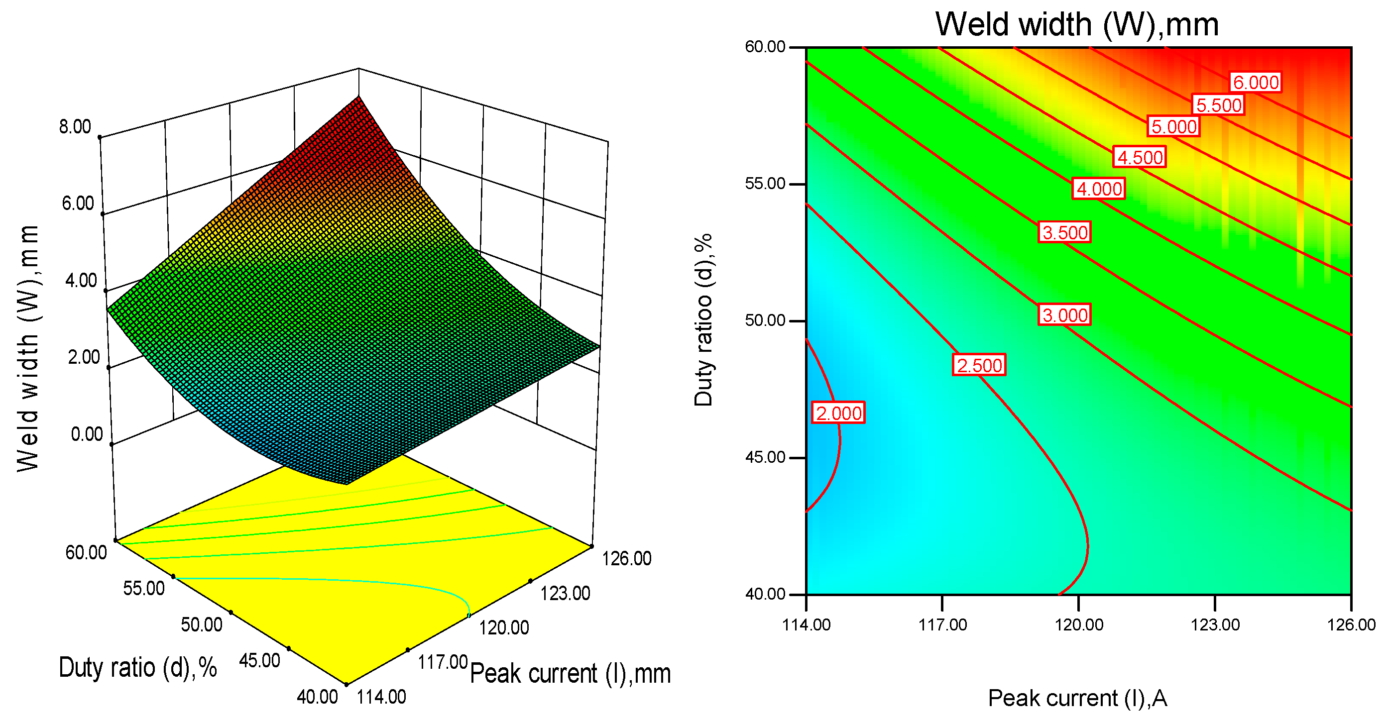
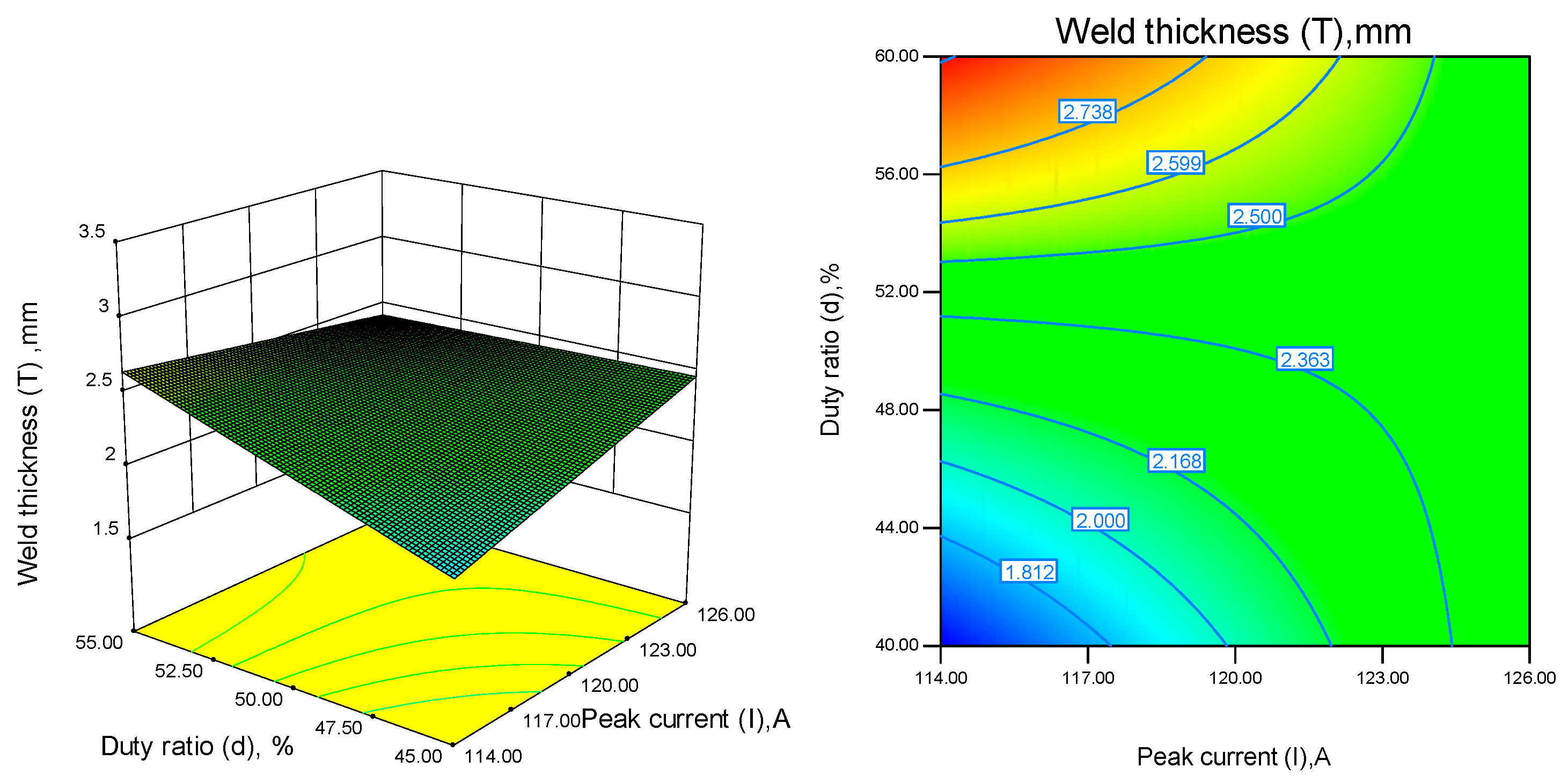
5.1. Influences of Welding Peak Current on Weld Width (W), Weld Depth (D), and Weld Thickness (T)

Considering the influence of the single factor welding peak current on the weld bead geometry, it can be shown from Figure 5 that the welding peak current increases with the increase in weld width, weld depth and weld thickness. This is because with weld peak current increasing leads to heat input increase per unit time, which is good for the weld metal melted and enhancing the deposition efficiency. As the peak current increases, the weld width and depth increase significantly, while weld thickness increases less. The weld thickness increases gradually from 2.331 to 2.436 mm with the increase in welding peak current from 114 to 126 A. This is because as the weld peak current increases, the arc force also increases, and the liquid metal is blown to both sides of the molten pool under the action of arc force, so the weld thickness increases indistinctly.

Figure 5. Influence of weld peak current on weld bead. (Welding velocity (V) = 63 mm/min, welding duty ratio (d) = 50%, welding position (P) = 90°).

5.2. Influences of Weld Velocity on W, D and T

Figure 6 indicates that the increase of welding velocity leads to the decrease in the heat input and volume of liquid filler metal per unit time of the weld bead, so the weld width, the weld depth and the weld thickness are correspondingly reduced.

Figure 6. Influence of welding velocity on weld bead. (Welding peak current (I) = 120 A, d = 50%, P = 90°).

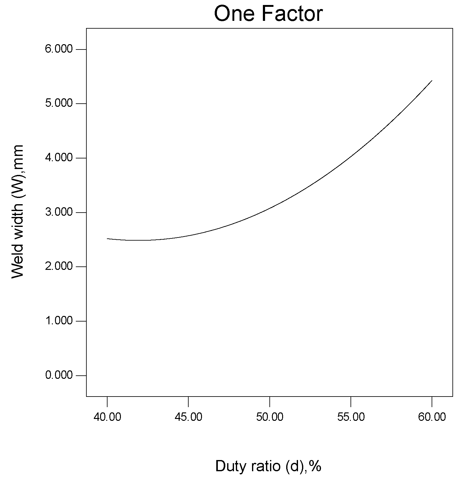
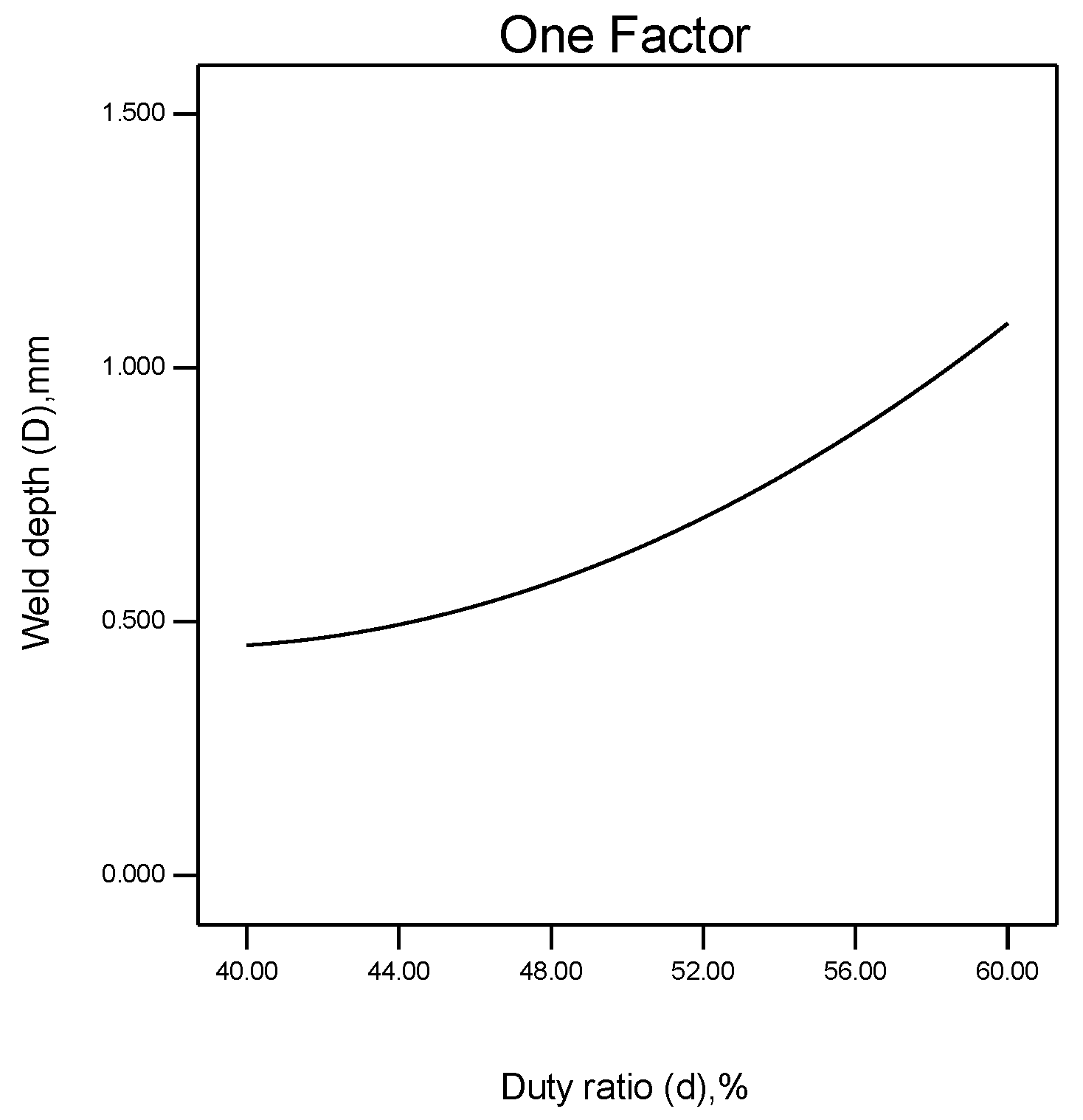
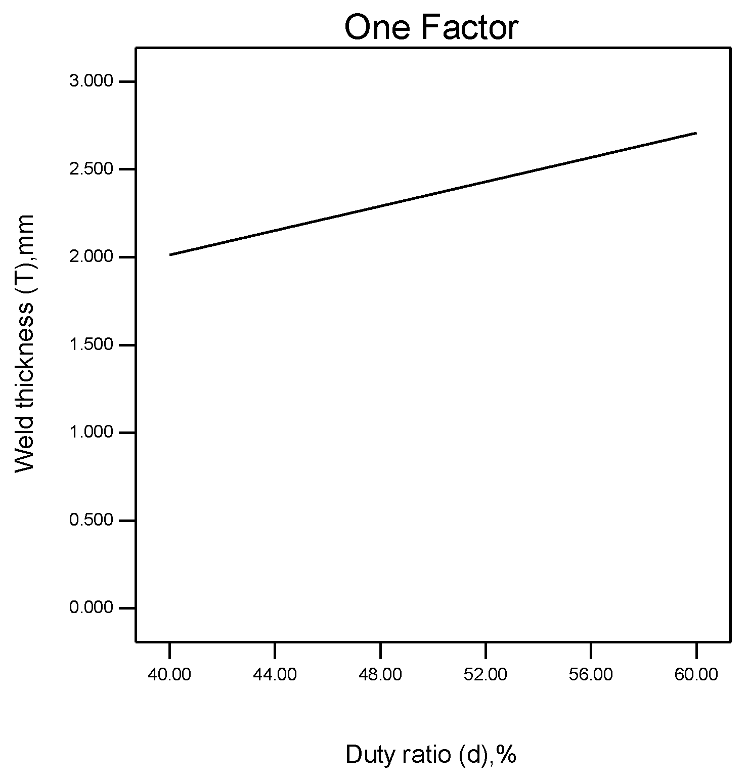
5.3. Effects of Duty Ratio on W, D and T

As shown in Figure 7, Figure 8 and Figure 9, as the duty ratio increases, the weld width, depth and thickness increase correspondingly. This is due to increases in the heat input and volume of the liquid filler metal per unit time of the weld bead. The weld width and depth have a quadratic parabolic relationship with the duty ratio, and the slope of the curve growth is getting bigger and bigger. Because the duty ratio is increased, the weld heat input to the weld bead is larger and the more heat that is accumulated per unit time, the more favorable is the melting of the weld metal so the rate of weld width and weld depth growth is increasing. It can be seen from Figure 9 that the weld thickness increases linearly with increasing duty ratio, although the increase in duty ratio and the accumulation of welding heat contribute to the weld thickness, but excessive heat leads to liquid metal loss on the weld surface.

Figure 7. Influence of duty ratio on weld width.

Figure 8. Influence of duty ratio on weld depth.

Figure 9. Influence of duty ratio on weld thickness.

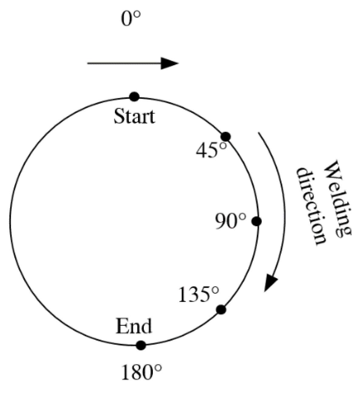
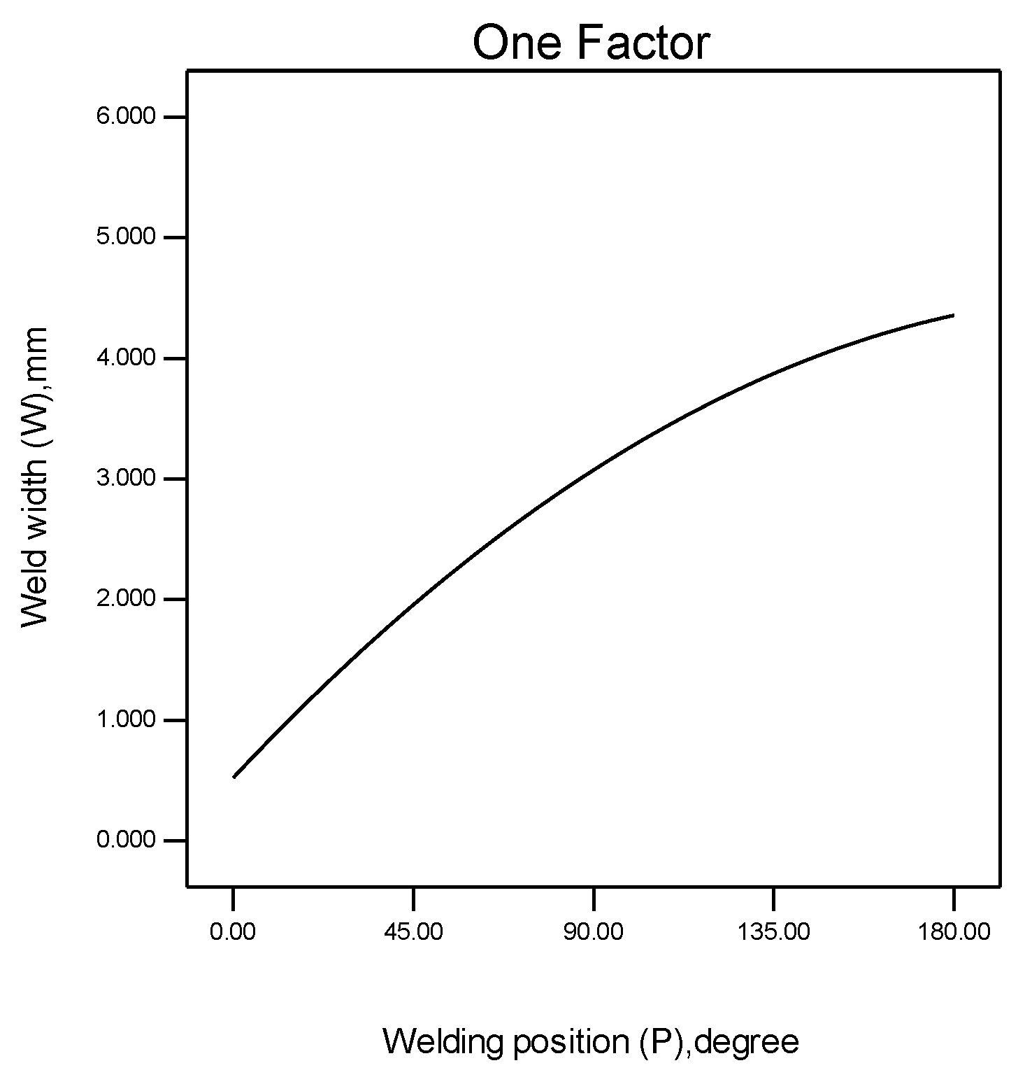
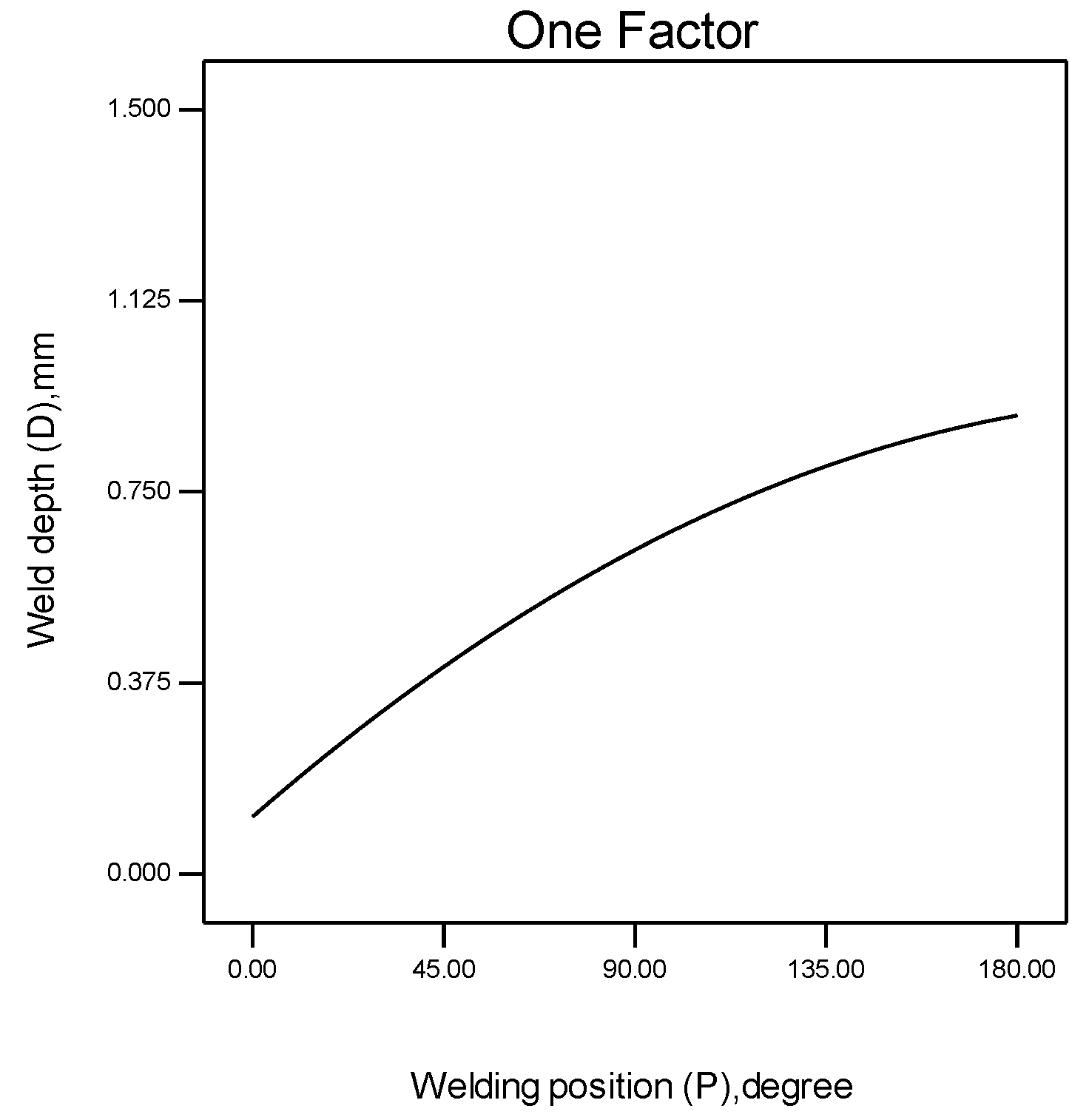
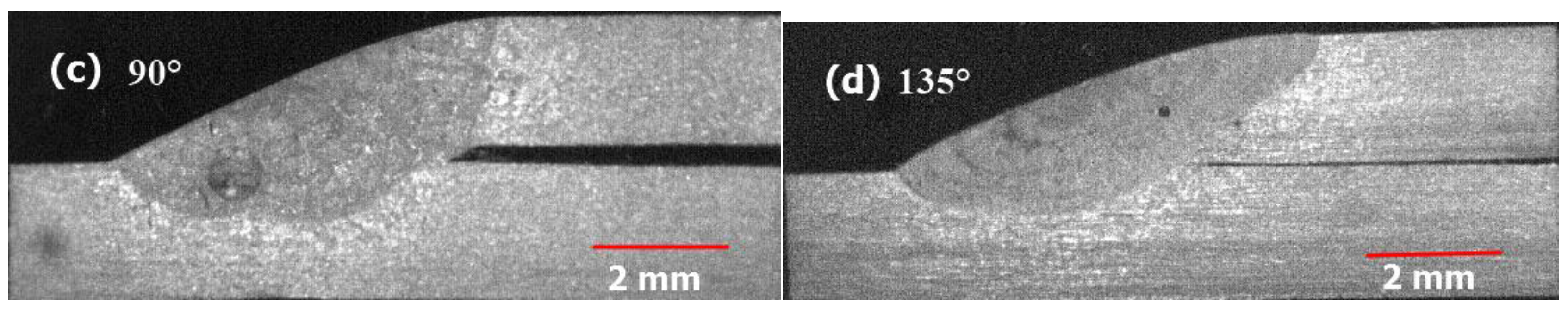
5.4. Effects of Welding Position on W, D and T

As shown in Figure 10 and Figure 11, as the degree of welding position increases, the weld width and weld depth increase correspondingly in the welding interval of 0–180°. The weld width and weld depth have a quadratic parabolic relationship to the degree of welding position, and the slope of the curve is getting smaller and smaller due to the gravity of the molten pool and the flow of molten metal along the weld bead during welding. Figure 12 shows the weld thickness increases first and then decreases. The gravity of the molten pool at different welding positions was shown in Figure 13. It was decomposed into a tangential force Gt and a radial force Gr. When welding in the 0–180° interval, the molten pool is subjected to the tangential force Gt, which leads to the molten liquid metal flowing down along the weld bead, and the flowing liquid metal can preheat the remaining weld bead and fill the weld bead, so the shape parameters of the weld width, weld depth and the weld thickness will increase with the increasing of the welding position degree. But when welding is in the 0–90°interval, the molten pool is subjected to the radial force Gr, and Gr = G cosθ. As the degree of the welding position increases, the radial force becomes smaller and smaller, and the direction of the radial force points to the center of the pipe; In the 90–180° interval welding, the molten pool is subjected to the direction of the radial force back to the center of the pipe, and Gr = G sin(θ − 90); with the welding position degree increasing, Gr becomes larger and larger, hindering the increase in weld width, depth and thickness. Therefore, the slope of the curve growth is getting smaller and smaller. Figure 12 shows the peak value of weld thickness for all values of P is received when P is 116°.

Figure 10. Influence of welding position on weld width.

Figure 11. Influence of welding position on weld depth.

Figure 12. Influence of welding position on weld thickness.

Figure 13. Gravity of molten pool at different welding positions.

5.5. Effects of Two-Factor Interaction on W, D and T

The interaction of I and d are shown in Figure 14, Figure 15 and Figure 16. The speed of the increase in W and D with the increases in I increases as d increases, and the speed of the increase in W and D with d increases as I increases. This is because that I and d have an active influence on heat input of the weld width and depth. In Figure 16, T increases as I increases when d is less than 50%, while it decreases as I increases when d is more than 50%.

Figure 14. Interaction of peak current and duty ratio on weld width.

Figure 15. Interaction of peak current and duty ratio on weld depth.

Figure 16. Interaction of peak current and duty ratio on weld thickness.

The interaction of I and P are shown in Figure 17 and Figure 18. The rate of the increase in W and D with the increases in I increases gradually as P increases, and the speed of increase in W and D with P increases as I increases.

Figure 17. Interaction of peak current and welding position on weld width.

Figure 18. Interaction of peak current and welding position on weld depth.

According to Figure 19, when the welding velocity is small, the T increases with the increase of the duty ratio. As the welding velocity increases, the influence of the duty ratio on T becomes smaller and smaller, because the welding velocity is large and the time of the welding process is short, so the welding heat input and the accumulated welding heat is small. When the duty ratio is small, the welding velocity has little effect on T. When the duty ratio is greater than the critical value, T decreases as the welding velocity increases.

Figure 19. Interaction of weld velocity and duty ratio on weld thickness.

5.6. Optimization of the Welding Parameters by Numerical Method

In order to obtain the ideal weld bead shape and avoid welding defects such as incomplete penetration and weld collapse, numerical analysis was used to optimize the welding parameters. The goal, lower, upper limits and importance for every input and response parameters of the standard are shown in Table 8. Table 9 lists optimal welding parameters at 0, 45°, 90°, 135° and 180° welding position. The Figure 20 has shown the cross sections of weld bead with the optimal parameters at disparate welding position in 0–180°, it shows that the gap between tubes is different for each case; there are two factors lead to this phenomenon. One factor is welding deformation: the welding process generates a lot of heat, which lead to pipes deformation. The other factor is welding sequence: welding experiments weld the bead at the 0° position firstly, so the weld bead was solidified first at the 0° welding position, which results in other gaps between tubes being confirmed.

Table 8. Restraint of numerical optimization.

Name	Goal	Lower	Upper	Importance
I	Is in range	114	126	3
V	Is in range	57	69	3
d	Is in range	40	60	3
P	Is equal to	0	180	3
W	maximize	0.987	5.859	5
D	Is in range	0.8	1.5	5
T	Is in range	1.533	3.204	5

Table 9. Optimal parameters.

I (A)	V (mm/min)	d (%)	P (Degree)
126	57	60	0
125	58	59	45
124	60	58	90
122	60	54	135
119	61	54	180

Figure 20. Cross sections of weld bead at different welding position from 0–180°. (a) 0° welding position, (b) 45° welding position, (c) 90° welding position, (d) 135° welding position.

6. Conclusions

In this research, the all-position automatic welding of pipes has been researched and statistically analysed. The main conclusions drawn from this research are as follows:

(1)

Response surface methodology (RSM) based on center composed design (CCD) can be used to establish a mathematical model, and it can predict weld bead shape in the all-position automatic welding of pipes.

(2)

Weld peak current had a prominent active influence on the important weld bead geometry parameters, while welding velocity had a negative influence on the important weld bead geometry parameters. The duty ratio exhibits a quadratic parabolic relationship with W and D, and the slope of the curve increases as the duty ratio increases, while T and the duty ratio increase linearly. The welding position has a quadratic parabolic relationship with the important weld bead geometry parameters, and the slope of the curve decreases as the degree of the welding position increases.

(3)

The ideal weld bead geometry can be obtained by choosing the optimal weld parameters with the established statistical models, and this model can be used for the all-position automatic welding of pipes.

References

1. Xu, W.H.; Lin, S.B.; Fan, C.L.; Zhuo, X.Q.; Yang, C.L. Statistical modelling of weld bead geometry in oscillating arc narrow gap all-position GMA welding. Int. J. Adv. Manuf. Technol. 2014, 72, 1705–1716. [Google Scholar] [CrossRef]
2. Manonmani, K.; Murugan, N.; Buvanasekaran, G. Effects of process parameters on the bead geometry of laser beam butt welded stainless steel sheets. Int. J. Adv. Manuf. Technol. 2007, 32, 1125–1133. [Google Scholar] [CrossRef]
3. Kim, D.I.S.; Basu, A.; Siores, E. Mathematical models for control of weld bead penetration in the GMAW process. Int. J. Adv. Manuf. Technol. 1996, 12, 393–401. [Google Scholar] [CrossRef]
4. Xu, W.H.; Lin, S.B.; Fan, C.L.; Yang, C.L. Prediction and optimization of weld bead geometry in oscillating arc narrow gap all-position GMA welding. Int. J. Adv. Manuf. Technol. 2015, 79, 183–196. [Google Scholar] [CrossRef]
5. Rao, P.S.; Gupta, O.P.; Murty, S.S.N.; Rao, A.B.K. Effect of process parameters and mathematical model for the prediction of bead geometry in pulsed GMA welding. Int. J. Adv. Manuf. Technol. 2009, 45, 496–505. [Google Scholar] [CrossRef]
6. Koleva, E. Electron beam weld parameters and thermal efficiency improvement. Vacuum 2005, 77, 413–421. [Google Scholar] [CrossRef]
7. Karthikeyan, R.; Balasubramanian, V. Predictions of the optimized friction stir spot welding process parameters for joining AA2024 aluminum alloy using RSM. Int. J. Adv. Manuf. Technol. 2010, 51, 173–183. [Google Scholar] [CrossRef]
8. Ii, E.J.L.; Torres, G.C.F.; Felizardo, I.; Filho, F.A.R.; Bracarense, A.Q. Development of a robot for orbital welding. Ind. Robot 2005, 32, 321–325. [Google Scholar]
9. Acherjee, B.; Kuar, A.S.; Mitra, S.; Misra, D. Modeling and analysis of simultaneous laser transmission welding of polycarbonates using an FEM and RSM combined approach. Opt. Laser Technol. 2012, 44, 995–1006. [Google Scholar] [CrossRef]
10. Gunaraj, V.; Murugan, N. Application of response surface methodology for predicting weld bead quality in submerged arc welding of pipes. J. Mater. Process. Technol. 1999, 88, 266–275. [Google Scholar] [CrossRef]
11. Acherjee, B.; Misra, D.; Bose, D.; Venkadeshwaran, K. Prediction of weld strength and seam width for laser transmission welding of thermoplastic using response surface methodology. Opt. Laser Technol. 2009, 41, 956–967. [Google Scholar] [CrossRef]
12. Ruggiero, A.; Tricarico, L.; Olabi, A.G.; Benyounis, K.Y. Weld-bead profile and costs optimisation of the CO2 dissimilar laser welding process of low carbon steel and austenitic steel AISI316. Opt. Laser Technol. 2011, 43, 82–90. [Google Scholar] [CrossRef]
13. Gunaraj, V.; Murugan, N. Prediction and comparison of the area of the heat-affected zone for the bead-on-plate and bead-on-joint in submerged arc welding of pipes. J. Mater. Process. Technol. 1999, 95, 246–261. [Google Scholar] [CrossRef]
14. Murugan, N.; Gunaraj, V. Prediction and control of weld bead geometry and shape relationships in submerged arc welding of pipes. J. Mater. Process. Technol. 2005, 168, 478–487. [Google Scholar] [CrossRef]
15. Rajakumar, S.; Balasubramanian, V. Diffusion bonding of titanium and AA7075 aluminum alloy dissimilar joints—Process modeling and optimization using desirability approach. Int. J. Adv. Manuf. Technol. 2016, 86, 1–18. [Google Scholar] [CrossRef]
16. Colombini, E.; Sola, R.; Parigi, G.; Veronesi, P.; Poli, G. Laser quenching of ionic nitrided steel: Effect of process parameters on microstructure and optimization. Metall. Mater. Trans. A 2014, 45, 5562–5573. [Google Scholar] [CrossRef]
17. Poli, G.; Sola, R.; Veronesi, P. Microwave-assisted combustion synthesis of NiAl intermetallics in a single mode applicator: Modeling and optimisation. Mater. Sci. Eng. A 2006, 441, 149–156. [Google Scholar] [CrossRef]
Article Metrics
Citations
Article Access Statistics
Multiple requests from the same IP address are counted as one view.