Trajectory Analysis of Copper and Glass Particles in Electrostatic Separation for the Recycling of ASR

Abstract

Automobile-shredder-residue (ASR) recycling techniques have been widely applied for improving the total recycling rate of end-of-life vehicles. In this study, to obtain useful information for predicting or improving ASR-separation efficiency, trajectory analyses of conductors (copper) and non-conductors (glass) were performed using a lab-scale induction electrostatic separator. The copper-wire trajectories obtained showed a good agreement depending significantly on the electric field strength and particle size. The observed copper-wire trajectories showed consistent congruity with the coarse-particles simulation (0.5 and 0.25 mm). The observed fine-particles (0.06 mm) trajectory was deflected toward the (−) attractive electrode, owing to the charge density effects due to the particle characteristics and relative humidity. This results in superior separation performance because more copper enters the conductor products bin. The actual dielectric-glass trajectory was deflected toward the (−) attractive electrode, thus showing characteristics similar to conductive-particle characteristics. Through analyses conducted using a stereoscopic microscope, scanning electron microscope, and energy dispersive spectroscope, we found heterogeneous materials (fine ferrous particles and conductive organics) on the glass surface. This demonstrates the separation-efficiency decrease for non-ferrous metals during electrostatic separation in the recycling of ASR. Future work should include a pretreatment process for eliminating impurities from the glass and advanced trajectory-simulation processes.

1. Introduction

The recycling of automobile shredder residue (ASR) that is generated in the final process of end-of-life vehicles (ELVs) is an important issue in the recycling field. The amount of ASR is constantly increasing, owing to advances in the automobile industry, but it is mostly disposed of in landfills [1]. Development of a technique for separating ASR that can achieve a recycling ratio of over 95% for ELVs as well as solve the corresponding disposal problems is required [2,3,4]. Furthermore, in terms of policy in Korea, the recycling of ASR is promoted by resource circulation law [5].

ASR can be separated using a series of mineral-processing operations, such as comminution, air classification, magnetic separation, and/or electrostatic separation. Non-ferrous metals in the ASR may be recovered by electrostatic separation but, to date, the use of this method has not been common. Electrostatic separation has been widely used for recycling various electric and electronic wastes, such as printed circuit boards (PCBs), cables, and plastics, and has been used as well in the mineral industry [6,7,8,9].

Previous studies involving electrostatic separation have been focused on the types of separators and electrodes, particle characteristics, and numerical simulations, as shown in

Table 1. Previous research on particle trajectory.

Author	Sample	Type of Separator	Year
L. Dascalescu et al. [10]	Artificial Sample	Roll-type Corona Electrostatic Separator	1995
S. Vlad et al. [13]	none	Plate-type Electrostatic Separator	2001
S. Vlad et al. [14]	Artificial Sample	Plate-type Electrostatic Separator	2003
H. Labair et al. [16]	ABS 1, PVC 2	Free-Fall Electrostatic Separator	2017
G. Richard et al. [17]	Electric Cable Waste	Roll-type Electrostatic Separator	2017
G. Richard et al. [18]	Electric Cable Waste	Plate-type Electrostatic Separator	2017
J. Li [19]	PCB 3	Roll-type Electrostatic Separator	2008
H. Lu et al. [21]	PCB	Roll-type Electrostatic Separator	2008
J. Wu et al. [22]	PCB	Roll-type Electrostatic Separator	2009

¹ Acrylonitrile Butadiene Styrene, ² Polyvinyl Chloride, ³ Printed Circuit Board.

. On reviewing the published literature, it was found that L. Dascalescu et al. [10,11,12,13,14,15,16,17,18] reported that the separator type, shape of the electrode, as well as electric field strength and size of the particle could affect the behavior of the particle, based on the results obtained from numerical modeling. L. Dascalescu et al. [10,15] also showed that the particle trajectory of conductors in basic numerical modeling using a roll-type corona-electrostatic separator is similar to that in the photographic records. S. Vlad et al. [11,12,13,14] used numerical modeling analysis to predict the behavior of polyamide spheres and steel balls, by evaluating the electric field strength at the surface of the plate electrode in a slop-plate-type electrostatic separator. G. Richards et al. [17,18] evaluated the trajectory of bare copper strands (of 2–5 mm length and 0.8–1.6 mm diameter) contained in granular electric cable wastes as a function of three different high-voltage electrodes using a statistical program. Z. Xu et al. [19,20,21,22] simulated the trajectory of a particle as a function of the shape of the particle and investigated the effects of the separation efficiency of conductors on roll-type corona-electrostatic separation. Furthermore, they reported that in obtaining an accurate trajectory simulation, the trajectory model of the conductive particle (i.e., the PCB) was improved when air drag force and various charging situations were introduced.

However, there is little research regarding trajectory simulation and the type of electrostatic separators used for ASR samples. In this study, a lab-scale induction electrostatic separator unit is designed for conducting tests with ASR. This study is focused on estimating the behaviors of conductive and non-conductive particles through observation and simulation, and predicting the possibility of ASR separation while taking into consideration variables such as the electric field strength and particle size and characteristics in the trajectory simulation.

2. Theoretical Aspects

In electrostatic separation, particles leave the edges of positive electrodes and fall freely under the influence of gravitational force (${\mathrm{F}}_{\mathrm{g}}$), electrostatic force (${\mathrm{F}}_{\mathrm{e}}$) when moving toward the electrostatic electrode, and air drag force (${\mathrm{F}}_{\mathrm{d}}$), as shown in Figure 1.

The forces acting on the particle are given as:

$${\mathrm{F}}_{\mathrm{e}}=\mathrm{QE}$$

(1)

$${\mathrm{F}}_{\mathrm{g}}=\mathrm{mg}$$

(2)

$${\mathrm{F}}_{\mathrm{d}}=6\mathsf{\pi }\mathsf{\eta }\mathrm{rV}$$

(3)

where Q is the surface charge of the particle, E is the electric field strength, m is the mass of the particle, g is the acceleration due to gravity, η is the air drag coefficient ($1.85\times {10}^{-5}$ Ns·m⁻¹), r is the radius of the particle, and V is the velocity of the particle.

The surface charge of a particle is influenced by different particle shapes (sphere, cylinder, ellipsoid). When the particle shape is cylindrical, the saturation charge $({\mathrm{Q}}_{\mathrm{s}})$ is given by: [10,23]

$${\mathrm{Q}}_{\mathrm{s}}=2{\mathsf{\pi }\mathrm{r}}_{\mathrm{p}}{\mathrm{l}}_{\mathrm{p}}{\mathsf{\epsilon }}_0{\mathsf{\epsilon }}_{\mathrm{a}}\mathrm{E},$$

(4)

where ${\mathrm{r}}_{\mathrm{p}}$ is the particle radius, ${\mathrm{l}}_{\mathrm{p}}$ is the particle length, ${\mathsf{\epsilon }}_0(8.85\times {10}^{-12}$ F·m⁻¹) is the permittivity of the vacuum, and ${\mathsf{\epsilon }}_{\mathrm{a}}$ is the relative permittivity of the air.

The electrostatic force exerted on the particle and contacted onto the surface of a grounded electrode may be given as:

$${\mathrm{F}}_{\mathrm{e}}=0.715{\mathrm{Q}}_{\mathrm{s}}\mathrm{E}$$

(5)

However, when the distance between a particle and grounded electrode is over 5 times the particle’s radius (${\mathrm{r}}_{\mathrm{p}}$), the electric forces are given as:

$$F_e\cong Q_{s}E$$

(6)

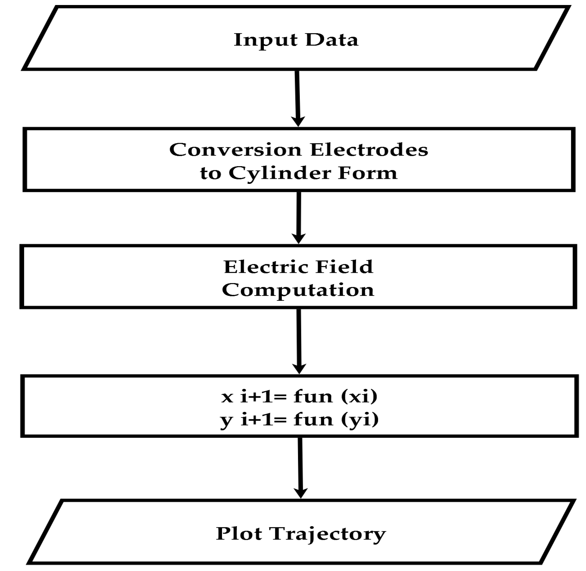
3. Computation Method

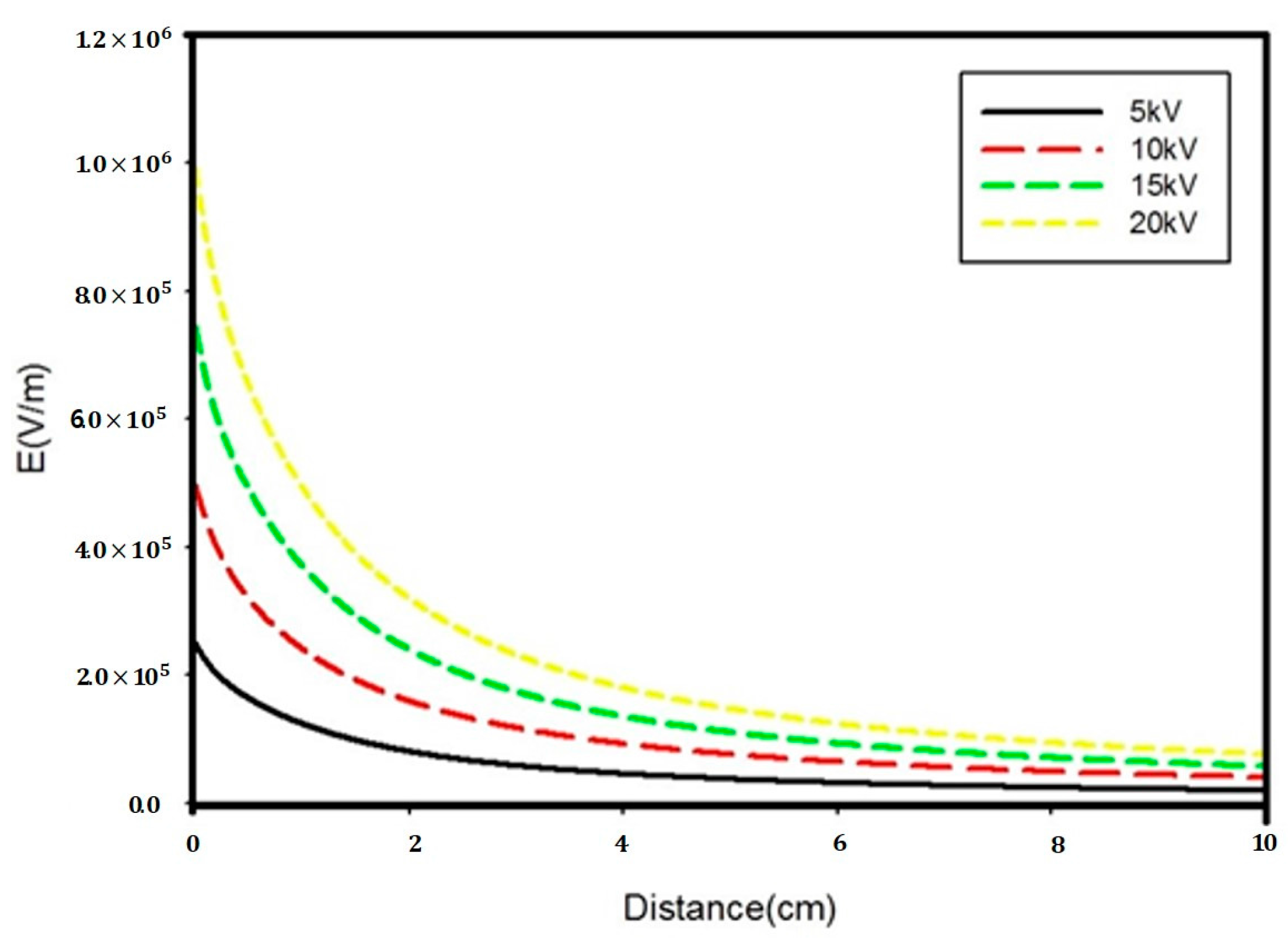
3.1. Calculation of Electric Field Strength

In electrostatic separation, electric field strength modeling is generally applied to cylindrical electrodes [15,19,20,21,22]. Hence, the plate electrodes were considered to be cylindrical, and the radii of these electrodes were given as:

$${\mathrm{r}}_{\mathrm{g}}={\mathrm{l}}_{\mathrm{g}}/\mathsf{\pi }$$

(7)

$${\mathrm{r}}_{\mathrm{e}}={\mathrm{l}}_{\mathrm{e}}/\mathsf{\pi },$$

(8)

where ${\mathrm{r}}_{\mathrm{g}}$ is the radius of the grounded cylindrical electrode, ${\mathrm{r}}_{\mathrm{e}}$ is the radius of the attractive cylindrical electrode, ${\mathrm{l}}_{\mathrm{g}}$ is a sectional length of the grounded plate electrode, and ${\mathrm{l}}_{\mathrm{e}}$ is a sectional length of the attractive plate electrode.

The model between the grounded cylindrical and attractive cylindrical electrodes proposed by J. Li [19] adapted the model equation for the electric field strength of two cylindrical electrodes proposed by S. Vlad et al. [24]. Its electric field strength is expressed in Equations (9)–(11):

$${\mathrm{E}}_{\mathrm{x}}=\mathrm{U}\times \mathsf{\delta }\times \left[\frac{\mathrm{j}-{\mathrm{h}}_1+{\mathrm{x}}_1}{{(\mathrm{j}-{\mathrm{h}}_1+{\mathrm{x}}_1)}^2+{\mathrm{y}}_1{}^2}+\frac{\mathrm{j}+{\mathrm{h}}_1-{\mathrm{x}}_1}{{(\mathrm{j}+{\mathrm{h}}_1-{\mathrm{x}}_1)}^2+{\mathrm{y}}_1{}^2}\right]$$

(9)

$${\mathrm{E}}_{\mathrm{y}}=\mathrm{U}\times \mathsf{\delta }\times \left[\frac{{\mathrm{y}}_1}{{(\mathrm{j}-{\mathrm{h}}_1+{\mathrm{x}}_1)}^2+{\mathrm{y}}_1{}^2}+\frac{{\mathrm{y}}_1}{{\left(\mathrm{j}+{\mathrm{h}}_1-{\mathrm{x}}_1\right)}^2+{\mathrm{y}}_1{}^2}\right]$$

(10)

$$\mathrm{E}=\sqrt{{\mathrm{E}}_{\mathrm{x}}{}^2+{\mathrm{E}}_{\mathrm{y}}{}^2},$$

(11)

where ${\mathrm{E}}_{\mathrm{x}}$ is the horizontal electronic field strength, ${\mathrm{E}}_{\mathrm{y}}$ is the vertical electronic field strength, E is the scalar value of the electronic field strength, and U is the applied high-voltage.

$${\mathrm{h}}_1=\frac{{\mathrm{L}}^2+{\mathrm{r}}_{\mathrm{g}}{}^2-{\mathrm{r}}_{\mathrm{e}}{}^2}{2\mathrm{L}}$$

(12)

$${\mathrm{h}}_2=\frac{{\mathrm{L}}^2-{\mathrm{r}}_{\mathrm{g}}{}^2+{\mathrm{r}}_{\mathrm{e}}{}^2}{2\mathrm{L}}$$

(13)

$$\mathrm{j}=\sqrt{{\mathrm{h}}_1{}^2-{\mathrm{r}}_{\mathrm{g}}{}^2}$$

(14)

$$\mathsf{\delta }=\ln \frac{\left({\mathrm{h}}_1+\mathrm{j}-{\mathrm{r}}_{\mathrm{g}}\right)\left({\mathrm{h}}_2+\mathrm{j}-{\mathrm{r}}_{\mathrm{e}}\right)}{\left({\mathrm{r}}_{\mathrm{g}}+\mathrm{j}-{\mathrm{h}}_1\right)\left({\mathrm{r}}_{\mathrm{e}}+\mathrm{j}-{\mathrm{h}}_2\right)}$$

(15)

$${\mathrm{x}}_1=\mathrm{x}\cos \left(\mathsf{\alpha }\right)+\mathrm{y}\sin \left(\mathsf{\alpha }\right)$$

(16)

$${\mathrm{y}}_1=\mathrm{y}\cos \left(\mathsf{\alpha }\right)-\mathrm{x}\sin \left(\mathsf{\alpha }\right),$$

(17)

where ${\mathrm{r}}_{\mathrm{g}}$ is the radius of the grounded cylindrical electrode, ${\mathrm{r}}_{\mathrm{e}}$ is the radius of the attractive cylindrical electrode, L is the distance between the axes of the grounded cylindrical and attractive cylindrical electrodes, and $\mathsf{\alpha }$ is the angle between the line of two axes and the horizontal line.

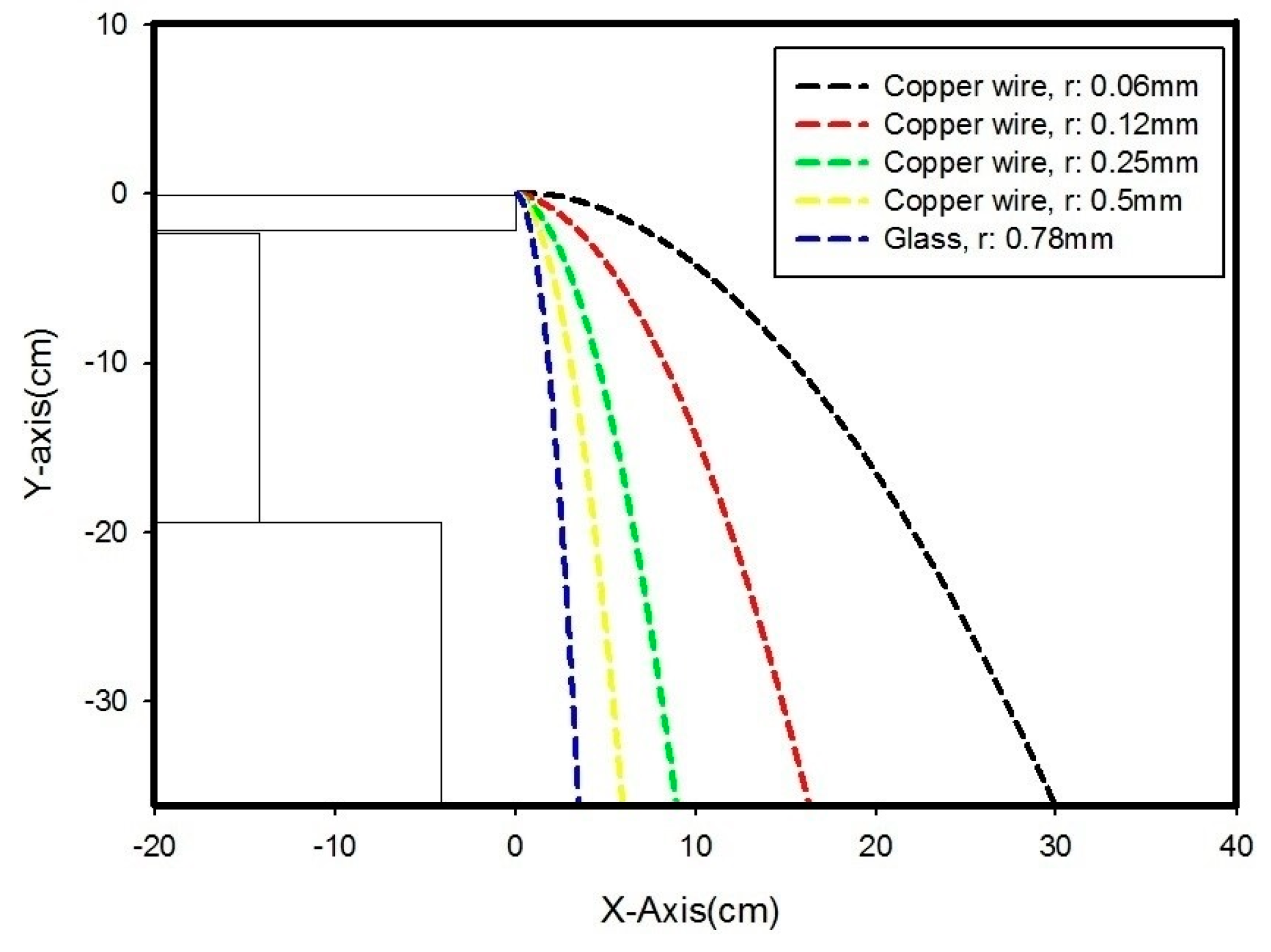
3.2. Particle Trajectory Computation

The computation methods in this study were conducted under the following assumptions:

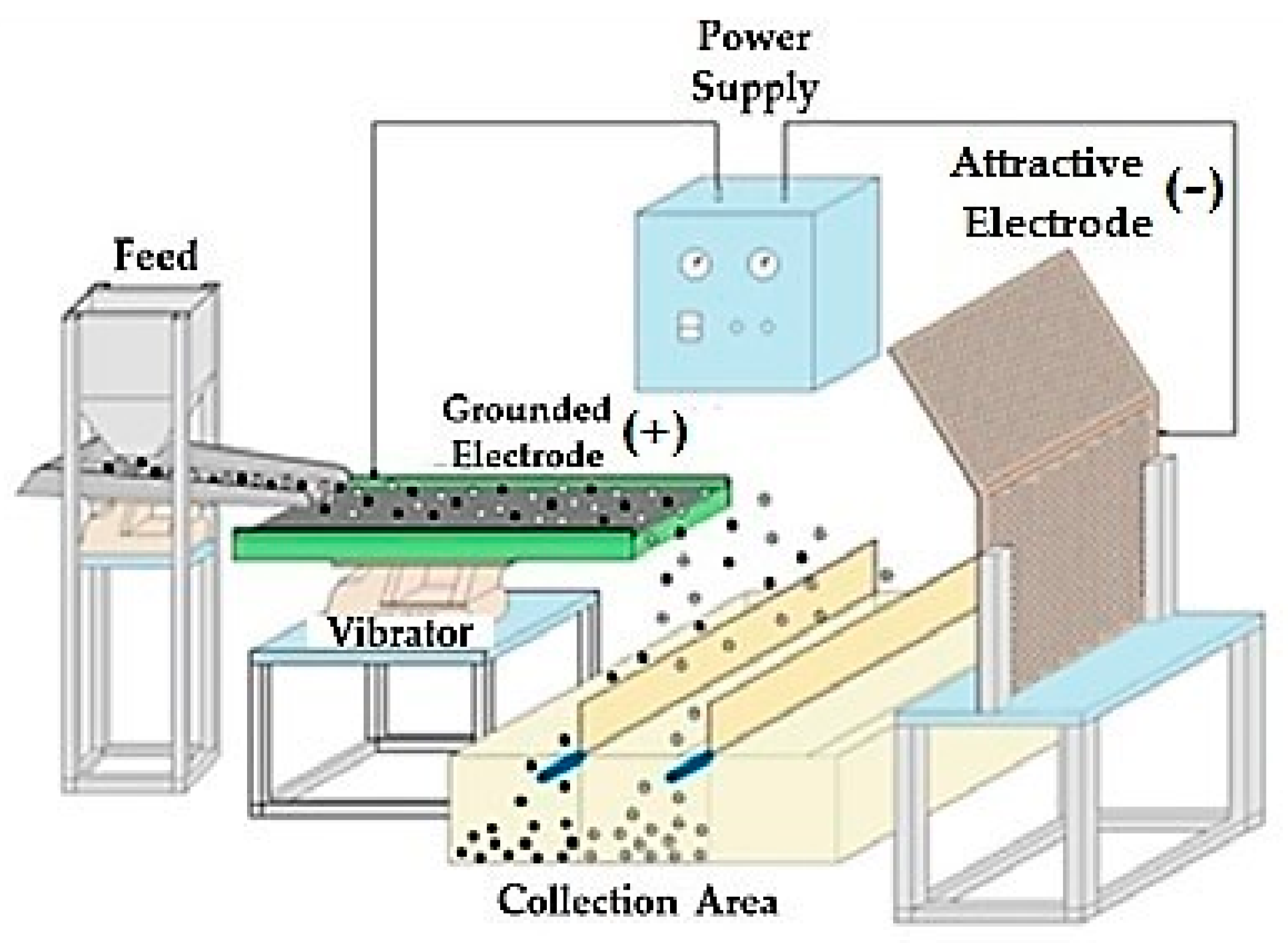
• The two electrodes are interpreted as being cylindrical.
• Particle shapes were a perfect cylinder or sphere model with a radius of (${\mathrm{r}}_{\mathrm{p}}$) and a density of (ρ).
• Particles were instantly charged using electrostatic induction with saturation charge.
• Depending on the particle shape, the saturation charge was calculated using Félici’s formula [23].
• The intervals between particles were large enough that the particles did not affect one another.
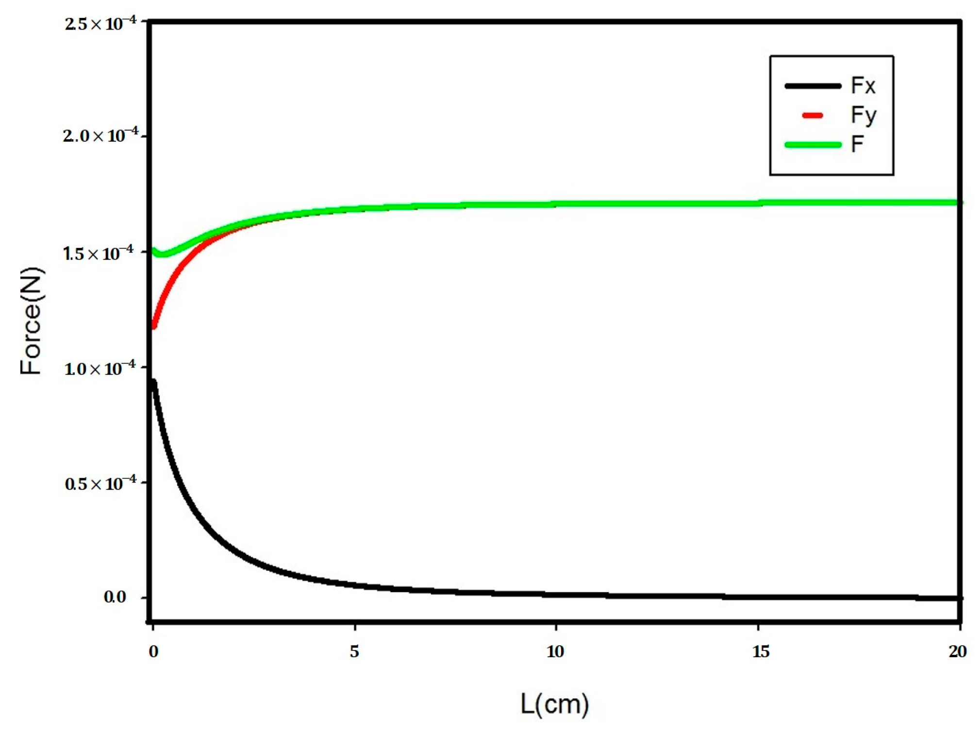
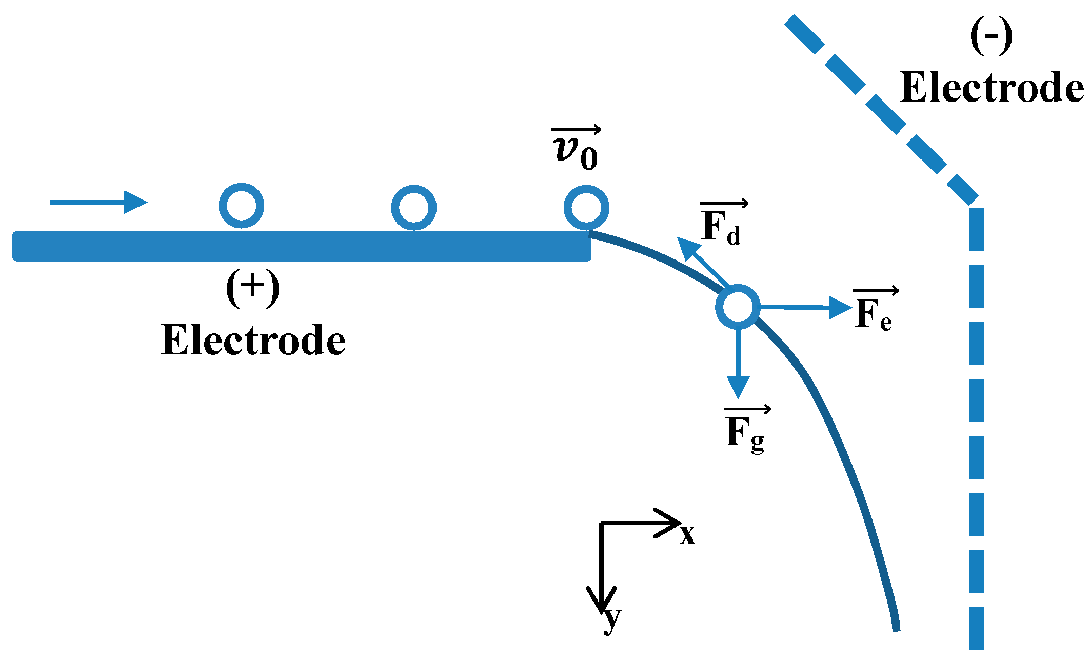
• The electric force before detachment is expressed as shown in Equation (5).
• The electric force after detachment is expressed as shown in Equation (6).
• The tribocharging effects between particles or between particle and electrode are ignored.

From Equations (1)–(3), the forces acting on the particle may be expressed as Equations (19) and (20). In addition, the horizontal and vertical components of the acceleration imparted on the particles are given in Equations (21) and (22):

$$\mathrm{F}=\sqrt{{\mathrm{F}}_{\mathrm{x}}{}^2+{\mathrm{F}}_{\mathrm{y}}{}^2}=\sqrt{{\mathrm{ma}}_{\mathrm{x}}{}^2+{\mathrm{ma}}_{\mathrm{y}}{}^2}$$

(18)

$${\mathrm{F}}_{\mathrm{x}}={\mathrm{F}}_{\mathrm{e}}-{\mathrm{F}}_{\mathrm{d}}$$

(19)

$${\mathrm{F}}_{\mathrm{y}}={\mathrm{F}}_{\mathrm{e}}+{\mathrm{F}}_{\mathrm{d}}-{\mathrm{F}}_{\mathrm{g}}$$

(20)

$${\mathrm{a}}_{\mathrm{x}}=\frac{{\mathrm{QE}}_{\mathrm{x}}-6{\mathsf{\pi }\mathsf{\eta }\mathrm{rV}}_{\mathrm{x}}}{\mathrm{m}}$$

(21)

$${\mathrm{a}}_{\mathrm{y}}=\frac{{\mathrm{QE}}_{\mathrm{y}}+6{\mathsf{\pi }\mathsf{\eta }\mathrm{rV}}_{\mathrm{y}}}{\mathrm{m}}-\mathrm{g}$$

(22)

Since the particle trajectory is a series of movements, trajectory is defined as an accumulation of particle movement in the minute time variation. The position of a particle as time variation is expressed as [17,19]:

$${\mathrm{x}}_{\mathrm{i}+1}={\mathrm{x}}_{\mathrm{i}}+{\mathrm{V}}_{\mathrm{x}}\left({\mathrm{x}}_{\mathrm{i}},{\mathrm{y}}_{\mathrm{i}}\right)\mathrm{dt}+0.5{\mathrm{a}}_{\mathrm{x}}\left({\mathrm{x}}_{\mathrm{i}},{\mathrm{y}}_{\mathrm{i}}\right){\mathrm{dt}}^2$$

(23)

$${\mathrm{y}}_{\mathrm{i}+1}={\mathrm{y}}_{\mathrm{i}}+{\mathrm{V}}_{\mathrm{y}}\left({\mathrm{x}}_{\mathrm{i}},{\mathrm{y}}_{\mathrm{i}}\right)\mathrm{dt}+0.5{\mathrm{a}}_{\mathrm{y}}\left({\mathrm{x}}_{\mathrm{i}},{\mathrm{y}}_{\mathrm{i}}\right){\mathrm{dt}}^2$$

(24)

Using the same approach, the particle velocity ($\mathrm{V}\left({\mathrm{x}}_{\mathrm{i}},{\mathrm{y}}_{\mathrm{i}}\right)$) in Equations (23) and (24) was obtained using the accumulation of the products of acceleration and time variation:

$${\mathrm{V}}_{\mathrm{x}}\left({\mathrm{x}}_{\mathrm{i}},{\mathrm{y}}_{\mathrm{i}}\right)={\mathrm{V}}_{\mathrm{x}}\left({\mathrm{x}}_{\mathrm{i}-1},{\mathrm{y}}_{\mathrm{i}-1}\right)+{\mathrm{a}}_{\mathrm{x}}\left({\mathrm{x}}_{\mathrm{i}-1},{\mathrm{y}}_{\mathrm{i}-1}\right)\mathrm{dt}$$

(25)

$${\mathrm{V}}_{\mathrm{y}}\left({\mathrm{x}}_{\mathrm{i}},{\mathrm{y}}_{\mathrm{i}}\right)={\mathrm{V}}_{\mathrm{y}}\left({\mathrm{x}}_{\mathrm{i}-1},{\mathrm{y}}_{\mathrm{i}-1}\right)+{\mathrm{a}}_{\mathrm{y}}\left({\mathrm{x}}_{\mathrm{i}-1},{\mathrm{y}}_{\mathrm{i}-1}\right)\mathrm{dt}$$

(26)

$${\mathrm{a}}_{\mathrm{x}}\left({\mathrm{x}}_{\mathrm{i}},{\mathrm{y}}_{\mathrm{i}}\right)=\frac{{\mathrm{QE}}_{\mathrm{x}}\left({\mathrm{x}}_{\mathrm{i}-1},{\mathrm{y}}_{\mathrm{i}-1}\right)-6{\mathsf{\pi }\mathsf{\eta }\mathrm{rV}}_{\mathrm{x}}\left({\mathrm{x}}_{\mathrm{i}-1},{\mathrm{y}}_{\mathrm{i}-1}\right)}{\mathrm{m}}$$

(27)

$${\mathrm{a}}_{\mathrm{y}}\left({\mathrm{x}}_{\mathrm{i}},{\mathrm{y}}_{\mathrm{i}}\right)=\frac{{\mathrm{QE}}_{\mathrm{y}}\left({\mathrm{x}}_{\mathrm{i}-1},{\mathrm{y}}_{\mathrm{i}-1}\right)+6{\mathsf{\pi }\mathsf{\eta }\mathrm{rV}}_{\mathrm{y}}\left({\mathrm{x}}_{\mathrm{i}-1},{\mathrm{y}}_{\mathrm{i}-1}\right)}{\mathrm{m}}-\mathrm{g}$$

(28)

As mentioned in Section 2 and Section 3, the complete computation process for particle trajectory in induction electrostatic separation can expressed as shown in Figure 2. Thus, particle trajectory may finally be plotted using Equations (23) and (24).

4. Materials and Methods

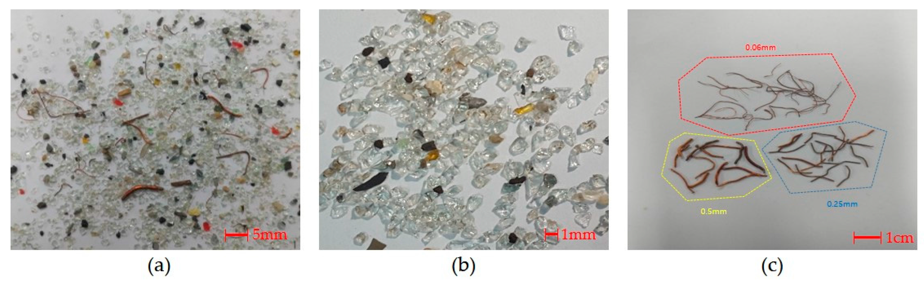
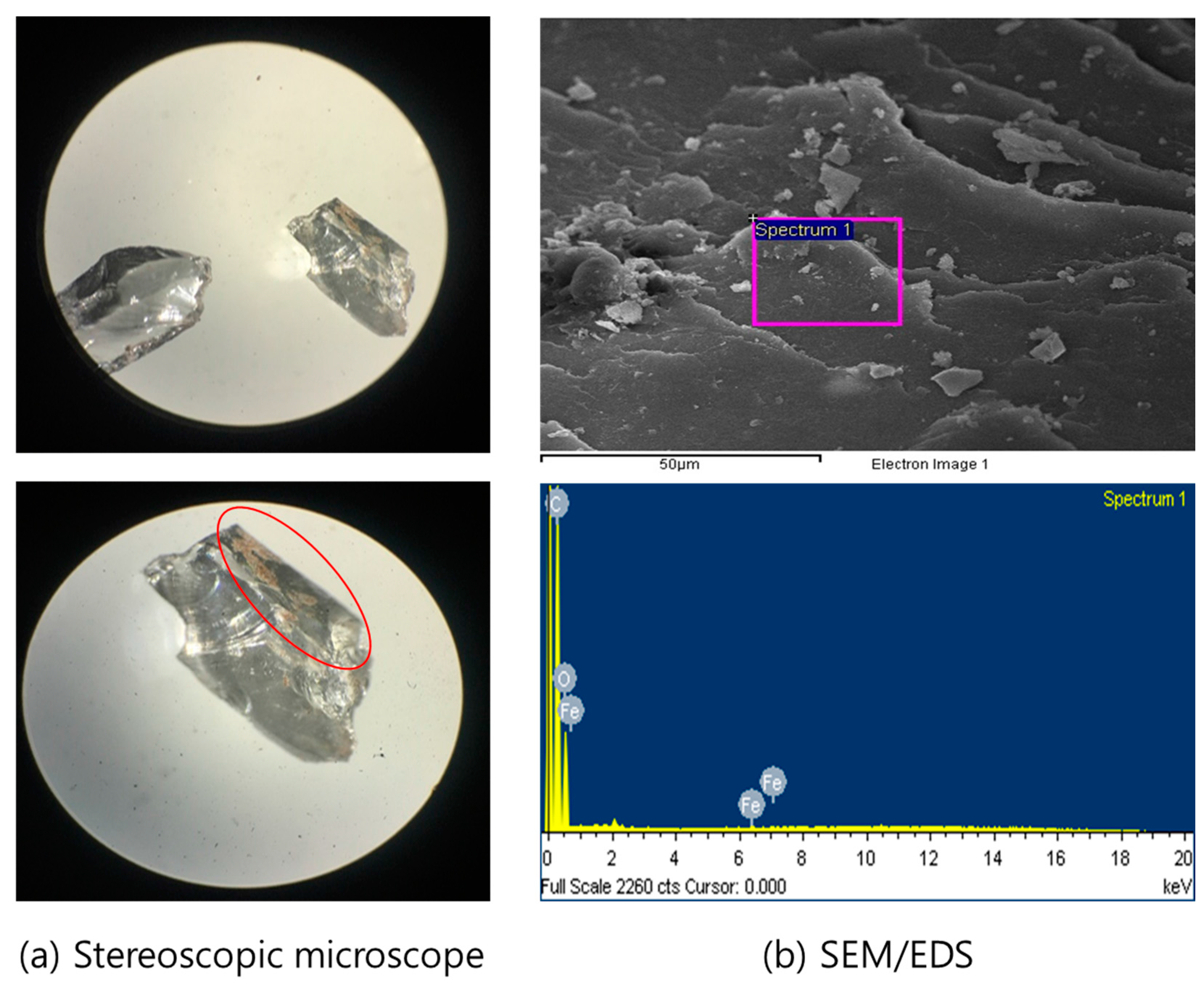
4.1. Materials

The samples used in this study were non-magnetic products separated from ASR using air classification and magnetic separation, and collected from Kyunghan Inc., located in Pohang, Korea. The ASR samples used in this study were as follows: (a) ASR, (b) glass, (c) copper wire. These samples are shown in Figure 3. The non-magnetic products consisted of 10% conductors (copper) and 90% non-conductors (glass, plastics, etc.). Copper and glass were chosen as the representative materials of each group for numerical modeling of the behavior of conductive and non-conductive particles.

4.2. Methods

A schematic of the lab-scale induction electrostatic separator set used in this study is shown in Figure 4. Copper wire and glass were fed onto the (+) electrode ground plate. The positively charged copper particles were deflected to the (−) electrode via the electric field between each electrode, and the glass particles then entered a free-fall. Thus, the conductor and non-conductor particles were separated by a splitter. The conditions of the variables of the experiments and simulations are shown in

Table 2. Conditions of experiment and simulation variables in particle trajectory.

Experimental Conditions
Feed rate (g·min−1)			50
Temperature (°C)			29
Humidity (%)			35–45
Initial Speed (m·s−1)			0.13
High Voltage (kV)			5, 10, 15, 20
Distance between Two Electrodes (m)			0.6
Particle Size	Copper	Diameter (m)	0.00012, 0.0005, 0.001
		Length(m)	0.01
	Glass	Diameter(m)	0.00014

. A super high-speed camera (Mach-F340, Comart System Inc., Seoul, Korea) was used to capture the trajectories of each particle. A (+) electrode plate was made from rubber and carbon, and a (−) electrode was made from aluminum. The power supply (KSA-C.) used was a direct current power source (max.: ±40 kV), and relative humidity was controlled using a dehumidifier (SDH-LX200, Shinil Corp., Seoul, Korea).

Based on the computation methods described in Section 3, Microsoft Excel 2016 (Microsoft Inc., Redmond, WA, USA) was used to calculate the electric field in the separator and to simulate particle trajectories. Moreover, all the trajectories and graphs in this paper were plotted using SigmaPlot 10 (SYSTAT Inc., San Jose, CA, USA).

5. Results and Discussion

The particle trajectories for conductors and non-conductors during induction electrostatic separation were simulated using the procedures, under the conditions shown in Figure 2 and Table 2, and compared with those of our experiments. Electric field strength is one of the most important parameters that affects the behavior of conductive particles. Thus, the variation of electric field strength as a function of applied voltage corresponding to the distance from the edge of the (+) electrode during computation (Equations (9)–(11)) on particle trajectory is shown in Figure 5. As expected, the variation of electric field strength increased with an increase of applied voltage and it decreased as distance increased. The magnitude of forces acting on a conductive particle as horizontal distance is plotted in Figure 6, which shows that gravitational force (${\mathrm{F}}_{\mathrm{g}}$) was consistent while air drag force (${\mathrm{F}}_{\mathrm{d}}$) was negligible. Electrostatic force (${\mathrm{F}}_{\mathrm{e}}$) decreased as horizontal distance increased, as electrostatic force (${\mathrm{F}}_{\mathrm{e}}$) is proportional to electric field strength (as shown in Equation (1)). The horizontal component force (${\mathrm{F}}_{\mathrm{x}}$), vertical component force $\left({\mathrm{F}}_{\mathrm{y}}\right)$, and resultant forces (${\mathrm{F}}_{\mathrm{t}}$) of both components imparted on the particles were plotted using Equations (18)–(20), as shown in Figure 7. As shown in the graph, ${\mathrm{F}}_{\mathrm{x}}$ decreased gradually with increasing horizontal distance, while ${\mathrm{F}}_{\mathrm{t}}$ remained close to ${\mathrm{F}}_{\mathrm{y}}$. Owing to the combination of these two forces, the parabolic curve of the particle trajectory fell.

The results of the trajectory simulations for copper wires and glass are shown in Figure 8. The moving distance of copper wire increased with decreasing particle size (${\mathrm{r}}_{\mathrm{p}}$) from 0.5 mm to 0.06 mm, owing to the fact that ${\mathrm{F}}_{\mathrm{g}}$ was much smaller than ${\mathrm{F}}_{\mathrm{e}}$ and ${\mathrm{F}}_{\mathrm{d}}$ when particle sizes were minute (for large particles, ${\mathrm{F}}_{\mathrm{g}}$ was predominant). On the other hand, dielectric glass does not have a residual charge, thus was not deflected toward the (−) electrode and fell freely. The results of the trajectory simulations for copper wire as applied voltage are shown in Figure 9, which shows that the moving distance of copper wire increased as applied voltage (U) increased (from 10 kV to 30 kV). From the simulation results shown in Figure 7 and Figure 8, we see that particle trajectory depends significantly on electric field strength and particle size. Thus, based on the conditions shown in Table 2, the actual trajectories of conductors (copper wire) and non-conductors (glass) were compared with the trajectory simulations shown in

Table 3. Particle trajectory by observation vs. simulation.

Material	R (mm)	U (kV)	Experimental Observation (cm)						Computation (cm)
			1st	2nd	3rd	4th	5th	Ave.
Copper	0.06	5	4.3	4.7	4.8	4.9	5.7	4.88	4.72
		10	13.8	15.3	16.5	17.7	18.4	16.34	9.20
		15	30	34	35	40	40.5	35.9	18.06
		20	38.3	42	42.1	44	46	42.48	29.88
	0.25	5	3.9	4	3.9	4.1	4.3	4.04	3.80
		10	4.4	5	5.1	5.1	5.5	5.02	4.67
		15	5.7	6.2	6.1	6.3	6.8	6.22	6.31
		20	8	9	9	9.4	9.5	8.98	8.94
	0.5	5	0.2	1	2	2.6	2.5	1.66	3.66
		10	2.4	2.2	2.8	3.2	3	2.72	4.08
		15	4.5	4.2	4.3	3.8	2.8	3.92	4.82
		20	4.4	6	5	5	5.2	5.12	5.97
Glass	0.78	5	3.6	2.4	2.4	2.3	2	2.54	3.52
		10	3.1	3.2	3.6	3.8	4.2	3.58	3.52
		15	5.8	5.9	6.4	6.5	7.4	6.4	3.52
		20	8.7	9.2	10.7	11.5	12.2	10.46	3.52

.

The trajectories for copper wires by observation vs. simulation are plotted in Figure 10. The experimental conditions were as follows: length of copper wire (${\mathrm{l}}_{\mathrm{p}}$): 0.01 m, initial speed (${\mathrm{v}}_0$): 0.13 m·s⁻¹, relative humidity: 35–45%, temperature: 29 °C, and distance between two electrodes (L): 0.6 m (as shown in Table 2. As shown in Figure 8 (for copper wires of 0.5 and 0.25 mm), trajectories were quite similar using both experimentation and simulation. In contrast, for a copper wire of 0.06 mm, the trajectories under experimentation deviated from those of simulation. This may be owing to difference between the simulated cylindrical electrodes and actual electrodes, specifically that the trajectories during experimentation may have been deflected toward vertical plate electrodes. Furthermore, smaller particles may be sensitive to the influence of electrostatic force (${\mathrm{F}}_{\mathrm{e}}$) due to the increase of a specific surface area and charge density (nC·g⁻¹), as well as the effects of particle shape and relative humidity.

The trajectories of glass particles by observation vs. simulation are plotted in Figure 11. Here, experimental conditions were as follows: radius (${\mathrm{r}}_{\mathrm{p}}$): 0.00007 m, initial speed (${\mathrm{v}}_0$): 0.13 m·s⁻¹, relative humidity: 35–45%, temperature: 29 °C, and distance between two electrodes (L): 0.6 m. Results shown in Figure 11 revealed that curves of trajectories from experimental observation moved considerably to the right as the applied voltage (U) increased (from 5 kV to 20 kV), compared with those from the simulation. This indicates that dielectric glass actually deflected toward the vertical plate electrode under experimental conditions. It seems that glass has a behavior similar to that of conductive particles; such results can deteriorate the grade of a copper product by misplacing glass into the collection zone of a conductor.

Glass surface samples were analyzed using a stereoscopic microscope and scanning elector microscope (SEM) and energy dispersive X-ray spectroscopy (EDS) as shown in Figure 12a,b, respectively. The stereoscopic images in Figure 12a show heterogeneous materials attached to the surface of glass. The SEM image and EDS analysis shown in Figure 12b found C, O, and Fe elements in the heterogeneous material, implying that most of these are conductive materials. There is a strong possibility that heterogeneous materials such as fine ferrous particles and conductive organics produced by ASR shredding were mechanically attached to the surface of the glass. This demonstrates that glass decreases the separation efficiency of non-ferrous metals during electrostatic separation for recycling ASR. In future work, we will seek to further refine a trajectory simulation of ASR samples through this systematic approach. In addition, we plan to conduct pretreatment work (such as water washing and sieving) to remove impurities found in the glass in this study.

6. Conclusions

In this study, trajectory analysis was performed using an induction electrostatic separator to improve the separation efficiency of ASR in the field of recycling. From our analysis of the trajectory simulations of conductors (copper) and non-conductors (glass), we have concluded that the simulated trajectories of conductors (copper) corresponded favorably with their actual trajectory, as shown in our experimental results. However, the simulated trajectories of non-conductors (glass) did not. In the case of the former, the trajectories of copper wire by observation vs. simulation for coarse particles (0.5 and 0.25 mm) showed consistent congruity. However, the observed trajectory for fine particles (0.06 mm) was deflected toward the (−) attractive electrode, owing to variations in particle type and relative humidity, as well as the influence of electrostatic force (${\mathrm{F}}_{\mathrm{e}}$) due to the increase in the specific surface area and charge density (nC·g⁻¹). In the case of non-conductors, the actual trajectory of dielectric glass deflected toward the vertical plate electrode and was misplaced into the collection zone of the conductor, showing characteristics similar to those of conductive particles. Our analyses of stereoscopic microscope and SEM and EDS found heterogeneous materials such as fine ferrous particles and conductive organics on the surface of the glass. This demonstrates that glass decreased separation efficiency for non-ferrous metals during electrostatic separation for the recycling ASR. Future work will require a pretreatment process to remove impurities from the glass, along with advancements in trajectory simulation processes.

References

1. Cossu, R.; Lai, T. Automotive shredder residue (ASR) management: An overview. Waste Manag. 2015, 45, 143–151. [Google Scholar] [CrossRef] [PubMed]
2. Passarini, F.; Ciacci, L.; Santini, A.; Vassura, I.; Morselli, L. Aluminium flows in vehicles: Enhancing the recovery at end-of-life. J. Mater. Cycles Waste Manag. 2014, 16, 39–45. [Google Scholar] [CrossRef]
3. Santini, A.; Passarini, F.; Vassura, I.; Serrano, D.; Dufour, J.; Morselli, L. Auto shredder residue recycling: Mechanical separation and pyrolysis. Waste Manag. 2012, 32, 852–858. [Google Scholar] [CrossRef] [PubMed]
4. Miller, L.; Soulliere, K.; Sawyer-Beaulieu, S.; Tseng, S.; Tam, E. Challenges and alternatives to plastics recycling in the automotive sector. Materials 2014, 7, 5883–5902. [Google Scholar] [CrossRef] [PubMed]
5. Ministry of Envrionment of Korea. Available online: http://www.law.go.kr/lsInfoP.do?lsiSeq=188594&urlMode=engLsInfoR&viewCls=engLsInfoR#0000 (accessed on 30 August 2017).
6. Tripathy, S.K.; Ramamurthy, Y.; Kumar, C.R. Modeling of high-tension roll separator for separation of titanium bearing minerals. Powder Technol. 2010, 201, 181–186. [Google Scholar] [CrossRef]
7. Tilmatine, A.; Medles, K.; Bendimerad, S.-E.; Boukholda, F.; Dascalescu, L. Electrostatic separators of particles: Application to plastic/metal, metal/metal and plastic/plastic mixtures. Waste Manag. 2009, 29, 228–232. [Google Scholar] [CrossRef] [PubMed]
8. Wu, J.; Li, J.; Xu, Z. Electrostatic separation for recovering metals and nonmetals from waste printed circuit board: Problems and improvements. Environ. Sci. Technol. 2008, 42, 5272–5276. [Google Scholar] [CrossRef] [PubMed]
9. Park, C.H.; Jeon, H.S.; Yu, H.S.; Han, O.H.; Park, J.K. Application of electrostatic separation to the recycling of plastic wastes: Separation of PVC, PET, and ABS. Environ. Sci. Technol. 2007, 42, 249–255. [Google Scholar] [CrossRef]
10. Dascalescu, L.; Mizuno, A.; Tobazeon, R.; Atten, P.; Morar, R.; Iuga, A.; Mihailescu, M.; Samuila, A. Charges and forces on conductive particles in roll-type corona-electrostatic separators. IEEE Trans. Ind. Appl. 1995, 31, 947–956. [Google Scholar] [CrossRef]
11. Vlad, S.; Iuga, A.; Dascalescu, L. Modelling of conducting particle behaviour in plate-type electrostatic separators. J. Phys. D Appl. Phys. 2000, 33, 127. [Google Scholar] [CrossRef]
12. Vlad, S.; Mihailescu, M.; Rafiroiu, D.; Iuga, A.; Dascalescu, L. Numerical analysis of the electric field in plate-type electrostatic separators. J. Electrost. 2000, 48, 217–229. [Google Scholar] [CrossRef]
13. Vlad, S.; Urs, A.; Iuga, A.; Dascalescu, L. Premises for the numerical computation of conducting particle trajectories in plate-type electrostatic separators. J. Electrost. 2001, 51, 259–265. [Google Scholar] [CrossRef]
14. Vlad, S.; Iuga, A.; Dascalescu, L. Numerical computation of conducting particle trajectories in plate-type electrostatic separators. IEEE Trans. Ind. Appl. 2003, 39, 66–71. [Google Scholar] [CrossRef]
15. Caron, A.; Dascalescu, L. Numerical modeling of combined corona-electrostatic fields. J. Electrost. 2004, 61, 43–55. [Google Scholar] [CrossRef]
16. Labair, H.; Touhami, S.; Tilmatine, A.; Hadjeri, S.; Medles, K.; Dascalescu, L. Study of charged particles trajectories in free-fall electrostatic separators. J. Electrost. 2017, 88, 10–14. [Google Scholar] [CrossRef]
17. Richard, G.; Salama, A.R.; Medles, K.; Lubat, C.; Touhami, S.; Dascalescu, L. Experimental and numerical study of the electrostatic separation of two types of copper wires from electric cable wastes. IEEE Trans. Ind. Appl. 2017, 53, 3960–3969. [Google Scholar] [CrossRef]
18. Richard, G.; Touhami, S.; Zeghloul, T.; Dascalescu, L. Optimization of metals and plastics recovery from electric cable wastes using a plate-type electrostatic separator. Waste Manag. 2017, 60, 112–122. [Google Scholar] [CrossRef] [PubMed]
19. Li, J.; Lu, H.; Xu, Z.; Zhou, Y. A model for computing the trajectories of the conducting particles from waste printed circuit boards in corona electrostatic separators. J. Hazard. Mater. 2008, 151, 52–57. [Google Scholar] [CrossRef] [PubMed]
20. Li, J.; Xu, Z.; Zhou, Y. Theoretic model and computer simulation of separating mixture metal particles from waste printed circuit board by electrostatic separator. J. Hazard. Mater. 2008, 153, 1308–1313. [Google Scholar] [CrossRef] [PubMed]
21. Lu, H.; Li, J.; Guo, J.; Xu, Z. Movement behavior in electrostatic separation: Recycling of metal materials from waste printed circuit board. J. Mater. Process. Technol. 2008, 197, 101–108. [Google Scholar] [CrossRef]
22. Wu, J.; Li, J.; Xu, Z. An improved model for computing the trajectories of conductive particles in roll-type electrostatic separator for recycling metals from weee. J. Hazard. Mater. 2009, 167, 489–493. [Google Scholar] [CrossRef] [PubMed]
23. Félici, N.J. Forces et charges de petits objets en contact avec une électrode affectée ďun champ électrique. Rev. Gén. Elec. 1966, 75, 1145–1160. [Google Scholar]
24. Angelov, A.; Vereshyagin, I.; Yershov, V. Physical Basis at Electrostatic Separation; Moscow Geology Press: Moscow, Russia, 1983. [Google Scholar]
Figure 1. Forces acting on particles in electrostatic separation.
Metals 07 00434 g001
Figure 2. Flow chart of the particle trajectory computation.
Metals 07 00434 g002
Figure 3. Automobile-shredder-residue (ASR) samples used in this study: (a) ASR; (b) glass; (c) copper wire.
Metals 07 00434 g003
Figure 4. Schematic of a lab-scale induction electrostatic separator set.
Metals 07 00434 g004
Figure 5. Variation of electric field strength as a function of distance at the applied voltages.
Metals 07 00434 g005
Figure 6. Magnitude of forces acting on a conductive particle as horizontal distance. (Radius of copper wire ( r p ): 0.00025 m, length of copper wire ( l p ): 0.01 m, and applied voltage (U): 20 kV).
Metals 07 00434 g006
Figure 7. Magnitude of forces ( F x , F y , F t ) acting on a conductive particle as horizontal distance. (Radius of copper wire ( r p ): 0.00025 m, length of copper wire ( l p ): 0.01 m, and applied voltage (U): 20 kV).
Metals 07 00434 g007
Figure 8. Trajectory simulation by particle size for copper wires and glass. (Applied voltage (U): 20 kV initial speed ( v 0 ): 0.13 m·s−1, distance between two electrodes (L): 0.6 m).
Metals 07 00434 g008
Figure 9. Trajectory simulations as applied voltage. (Radius of copper wire ( r p ): 0.00025 m, length of copper wire ( l p ): 0.01 m, initial speed ( v 0 ): 0.13 m·s−1, distance between two electrodes (L): 0.6 m).
Metals 07 00434 g009
Figure 10. Comparison of conductive particle trajectory by observation vs. simulation. (Applied voltage (U): 20 kV, initial speed ( v 0 ): 0.13 m·s−1, distance between two electrodes (L): 0.6 m).
Metals 07 00434 g010
Figure 11. Comparison of non-conductive particle trajectory by observation vs. simulation. (Applied voltage (U): 20 kV, initial speed ( v 0 ): 0.13 m·s−1, distance between two electrodes (L): 0.6 m).
Metals 07 00434 g011
Figure 12. (a) Stereoscopic microscope of glass from ASR, (b) SEM and EDS of glass from ASR.
Metals 07 00434 g012