Article

Comparative Analysis of Various Supervised Machine Learning Models for the Prediction of the Outcome of the Welded Bead Bending Test


by
Fritz Backofen
*,
Ulrike Hähnel
,
Frank Hahn
and
Kristin Hockauf
Research Group Materials, Production, Quality, Faculty Engineering Sciences, Mittweida University of Applied Sciences, Technikumplatz 17, 09648 Mittweida, Germany
*
Author to whom correspondence should be addressed.
Metals 2026, 16(4), 418; https://doi.org/10.3390/met16040418
Submission received: 9 March 2026 / Revised: 31 March 2026 / Accepted: 8 April 2026 / Published: 10 April 2026
(This article belongs to the Section Computation and Simulation on Metals)

Abstract

The Welded Bead Bending Test (WBBT) assesses steel structures intended for construction in Germany in accordance with ZTV-ING Part 4 or DBS 918 002-02, as specified in Stahl-Eisen-Prüfblatt (SEP) 1390. Test outcomes are classified as passed (p) if the minimum bending angle α 60 is achieved without fracture, not passed (n.p.) if fracture occurs beforehand, and invalid if no crack propagates into the base material. This study evaluates eight supervised machine learning models for classification regarding their suitability for predicting WBBT results: Decision Tree Classifier (DT), Random Forest Classifier (RF), Histogram-based Gradient Boosting Classifier (HGBC), k-Nearest-Neighbour (KNN), Bagging Classifiers based on DT (BCDT) and RF (BCRF), Generalized Learning Vector Quantizer (GLVQ), and Generalized Matrix Learning Vector Quantizer (GMLVQ). An industrial dataset of approximately 3600 samples was compiled in collaboration with Chemnitzer Werkstoff und Oberflächentechnik GmbH (CEWUS). Evaluation metrics included Balanced Accuracy, Recall, Specificity, computation time, and prediction stability. BCDT and BCRF achieved the highest Balanced Accuracy (70.6% and 70.3%, respectively), with BCRF excelling in Specificity (82.5%), thereby reliably detecting the n.p. class. GLVQ and GMLVQ demonstrated superior stability (maximum variability between training and testing dataset 0.14% and 3.17%, respectively), while BCRF and GMLVQ required the longest training times (BCRF: 10 s–20 s; GMLVQ: up to 80 s). KNN proved least suitable for WBBT outcome prediction.

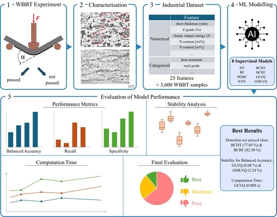
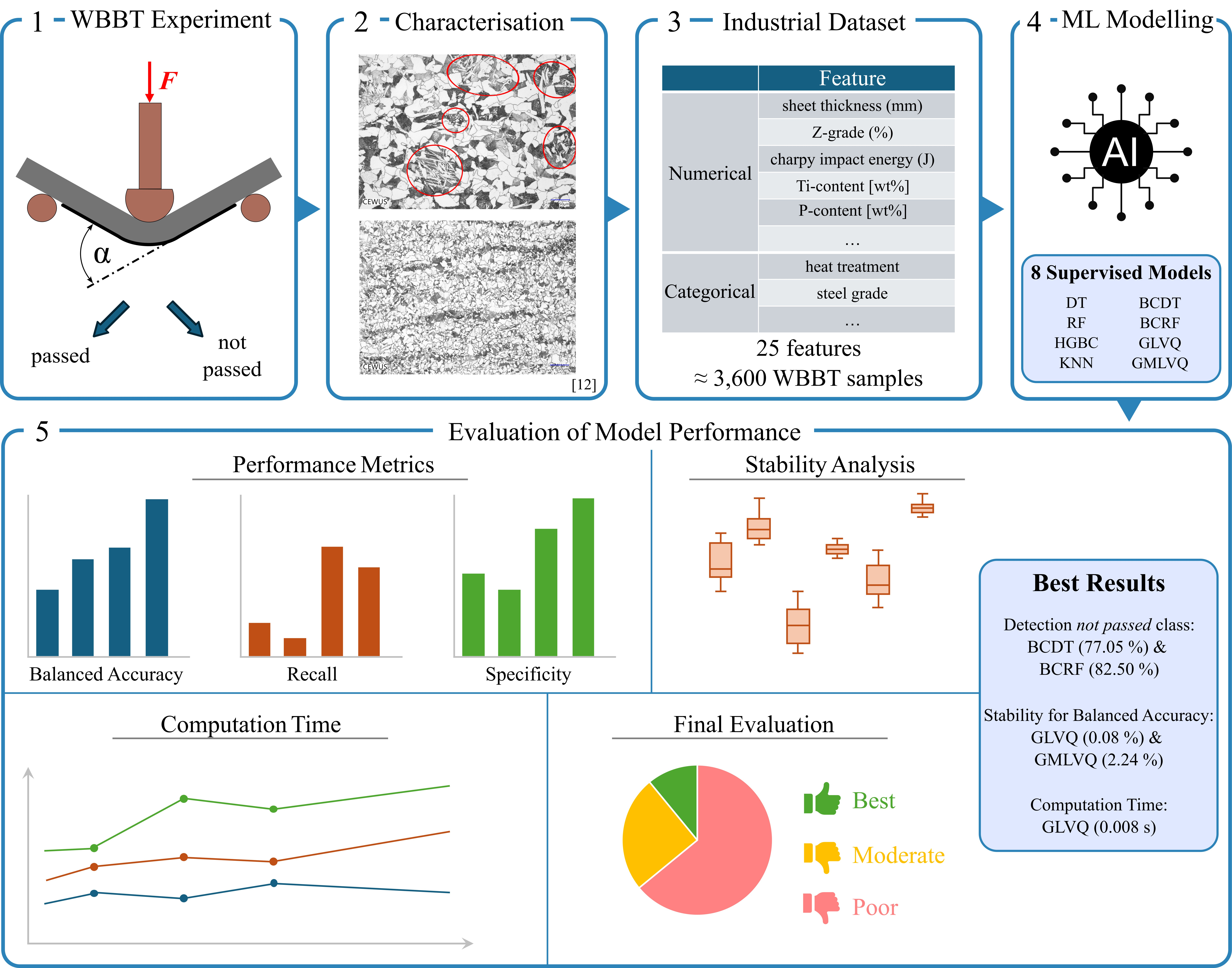
Graphical Abstract

1. Introduction

The utilisation of Artificial Intelligence (AI) and Machine Learning (ML) within materials science has accelerated considerably in recent years, ushering in marked improvements in the prediction of material properties, the optimisation of processes, and the advancement of high-performance materials. Through the integration of AI methodologies with experimental and computational approaches, researchers are able to systematically discern complex patterns within extensive datasets. A substantial number of studies have corroborated the value of such methodologies, including ML frameworks for fatigue-life prediction [1], AI-assisted advanced microstructural characterisation [2], and smart sensor systems for real-time monitoring of material behaviour [3]. Ensuring the safety of infrastructure, particularly that of bridges, constitutes both a technical obligation and a societal responsibility. Consequently, the qualification of construction materials is of primary importance. Within this context, the Welded Bead Bending Test (WBBT) represents a key component of the qualification process, serving as a benchmark for evaluating the suitability of structural steels employed in safety-critical applications. In Germany, steel structures designed in accordance with ZTV-ING Part 4 [4] or Deutsche Bahn Standard 918 002-02 [5] are required to demonstrate sufficient crack-arrest capability under deformation loading conditions. The WBBT, as specified in Stahl-Eisen-Prüfblatt (SEP) 1390 [6], provides a comprehensive framework for assessing a material’s resistance to crack propagation, particularly with regard to the transition of cracks from weld-induced stress zones into the base material. Historically, the WBBT was developed in the 1930s as a response to the recurring occurrence of cracks and brittle fractures in welded bridges across Germany [7]. Its primary objective was to devise a method for characterising the toughness of steel grades in welded sheets subjected to combined tensile and bending stresses. Despite its inherently empirical nature, the WBBT yields substantial insights into the mechanisms governing fracture behaviour, while deliberately deviating from fracture-mechanics-based formulations as its theoretical foundation. Within the framework of European standardisation, DIN EN 1993-1-1:2025-04 [8] (Eurocode 3) establishes the criteria for selecting steel grades on the basis of toughness and through-thickness properties. These are derived from fracture-mechanics principles and correlated with the transition temperature T 27 J , which is specific to the Charpy-V notch test. Despite its resource-intensive nature and categorisation as a technological test rather than one based on fracture mechanics, the WBBT maintains its indispensable role within the German context. For welded structures subjected to combined bending and tensile loading, the WBBT has proven more informative than the Charpy-V notch test, yet less demanding than comprehensive fracture-mechanics investigations. The WBBT classifies specimens as passed, not passed, or invalid depending on the crack propagation behaviour (see Section 2.1 for details). Previous research has sought to establish a relationship between the energy absorption in the Charpy-V notch test and WBBT outcomes [9,10]. As a consequence, DIN EN 1993 incorporates additional requirements concerning the toughness of base materials, consistent with the findings of Sedlacek et al. [10]. Nevertheless, despite notable progress in elucidating these relationships and clarifying the associated mechanisms, a definitive and comprehensive correlation remains elusive. Even though repeated endeavours have been made to develop a reliable yet simplified substitute for the complex WBBT, these efforts have thus far proven unsuccessful, highlighting the necessity of its continued implementation. Given the considerable costs associated with destructive testing, there is a growing incentive to explore alternative approaches that may enable the prediction of test outcomes using existing material data. In this context, employing ML techniques represents a promising avenue for the efficient evaluation of WBBT outcomes. Based on the predicted class probabilities and the overall model performance, steel manufacturers can make an informed preliminary decision on whether to submit a sample for WBBT certification. Nevertheless, it must be acknowledged that the efficacy of individual models is inherently dependent upon the structure of the underlying data. Consequently, a systematic comparison is required to assess their predictive capabilities and to ascertain how accurately WBBT outcomes can be anticipated. The present study presents a systematic evaluation of multiple ML classifiers aimed at predicting the outcomes of the WBBT. The analysis is based on an extensive dataset comprising approximately 3600 steel specimens with 25 numerical and categorical features, collected in collaboration with Chemnitzer Werkstoff und Oberflächentechnik GmbH (CEWUS, Chemnitz, Germany). Imputation procedures and data balancing techniques were employed to mitigate the pronounced sparsity and class imbalance (p/n.p.) observed within the dataset. The predictive capability of eight supervised ML classifiers was examined with reference to Balanced Accuracy, class-wise performance, computational efficiency, and model stability: Decision Tree Classifier (DT), Random Forest Classifier (RF), Histogram-based Gradient Boosting Classifier (HGBC), k-Nearest Neighbour (KNN), and Bagging Classifiers based on DT and RF (BCDT, BCRF). In addition, two learning vector quantisation approaches were investigated: the Generalized Learning Vector Quantizer (GLVQ) and the Generalized Matrix Learning Vector Quantizer (GMLVQ). A feature importance analysis was performed to identify the most influential variables driving the predictions of the WBBT outcome.

2. Materials and Methods

2.1. Welded Bead Bending Test (WBBT)

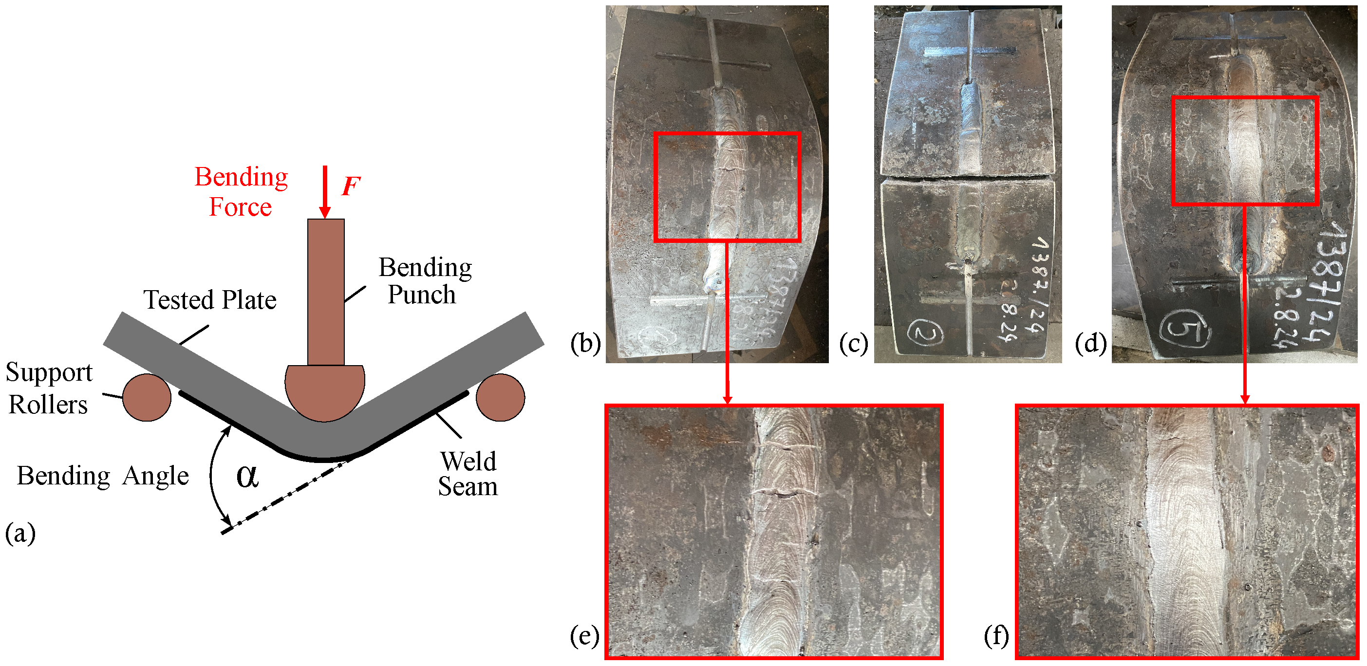
In Germany, the procedure for conducting the Welded Bead Bending Test (WBBT, “Aufschweißbiegeversuch”) is delineated by SEP 1390 [6]. Steel plates with a thickness ranging from 30 mm to 50 mm, a width of 200 mm, and a thickness-dependent length between 410 mm and 500 mm are selected for testing. The initial modification of these specimens involves the introduction of a groove using mechanical milling. This groove is subsequently filled with welding material (electrode type RR as defined by DIN EN ISO 2560 [11]) by means of manual electrode welding. Within the Heat-Affected Zone (HAZ), the thermal input during welding induces significant microstructural transformation, most notably the hardening of the steel in this region as a consequence of martensite formation. Following the welding operation, the test specimen is subjected to a three-point bending test, as schematically illustrated in Figure 1a. The reduced material’s inherent deformation capacity results in crack initiation during this process. Longitudinal macrosection examinations from earlier studies have unequivocally demonstrated that crack initiation occurs precisely within the HAZ, below the surface of the material [12]. Upon further bending, this crack propagates towards the surface and subsequently extends into the base material. There are three possible test outcomes: passed (Figure 1b,e) at α 60 without fracture but cracks extending from the HAZ into the base material, not passed (Figure 1c) at fracture with α < 60 and invalid (Figure 1d,f) if no crack, macroscopically visible from the exterior, has propagated from the HAZ into the base material.

2.2. Dataset

Significant parameters of the WBBT have been identified and established as features for modelling through a series of earlier material testing investigations [12]. The present study is based on this foundation, employing a comprehensive dataset compiled by CEWUS, comprising 25 parameters drawn from approximately 3600 samples. This dataset contains mixed data types, incorporating both categorical and numerical features as input variables. The former encompasses the delivery condition, the steel grade, and the rolling direction of the respective steel sheets. The numerical parameters considered include the material thickness (mm), the Charpy V-Notch impact energy (CVN) in joules (J), and the Z-grade (Z), which is defined as the reduction of area at fracture of the base material in the through-thickness direction, expressed as a percentage (%). For both CVN and Z, the corresponding standard deviations (std. dev.), based on three independent measurements, were also considered. Additionally, the mass percentages [wt%] of chemical elements such as carbon, manganese, and silicon were determined by optical emission spectrometry (OES). The output variable is the predicted class: passed (p) or not passed (n.p.) in the WBBT. Invalid test results were not considered in the assessment, as their use would have been inappropriate in order to evaluate material-related toughness. Two aspects of the dataset are worthy of note. Firstly, a strong imbalance is evident between the p and the n.p. class. The vast majority of specimens passed the WBBT. A mere 6.5% of the samples can be assigned to the n.p. class. Table 1 provides a detailed overview of this issue.
Moreover, for the majority of the specimens, merely a small number of the total 25 features were documented. For instance, the CVN has only been measured for approximately 20% of the samples. It is evident that, due to the measurement detection limit, values for As, B and Sn are only recorded for 4% to 8% of samples, rendering them particularly striking in terms of their sparsity. The complete range of implemented features and the proportion of samples for which the respective feature was recorded are displayed in Table 2. Consequently, it can be concluded that the overall dataset is imbalanced with regard to the classes and incomplete with regard to the features.

2.3. Models

The following eight classifiers were implemented: simple (DT and KNN), ensemble (RF, HGBC, BCDT, BCRF) and prototype-based (GLVQ, GMLVQ) models. The DT [13,14] recursively partitions the feature space using metrics such as information gain until a predefined depth or minimum node size is reached. Pruning techniques are utilised to mitigate the issue of overfitting. DT is characterised by its transparency and intuitive nature, which renders it advantageous to the processes of classification and regression. KNN [15] is a non-parametric, instance-based learning method. Predictions are derived from the majority class among the k nearest neighbours, determined by a distance measure. This approach exemplifies a form of lazy learning, characterised by its ability to perform computation exclusively during the prediction stage, thus bypassing the construction of an explicit training model. KNN is well-suited for multiclass classification but is costly for large datasets. The BCDT [16] combines multiple DTs trained on bootstrap samples of the dataset. The ensemble prediction is derived from the majority vote of individual trees. This bagging strategy has been demonstrated to reduce model variance and overfitting, thereby enhancing stability and predictive accuracy. The RF [17] extends the bagging method by incorporating random feature selection at each tree split, thus resulting in a diverse ensemble of DTs. As in BCDT, the final prediction is derived through majority voting among the individual models. RF demonstrates robustness, leading to a reduction in variance and a high degree of predictive stability, even in the presence of outliers. The BCRF [16] is an ensemble of multiple RFs, with each RF being trained on a bootstrap sample. The predictions are aggregated via majority voting in order to stabilise the results. The BCRF methodology integrates the strengths of bagging with the randomised feature selection of RF, thereby enhancing the accuracy and robustness of the resulting model. The HGBC [18] employs a sequential ensemble of weak learners, typically DTs, where each model corrects the residual errors of its predecessors. The application of histogram-based binning has been demonstrated to enhance computational efficiency by means of discretising continuous feature values. It is evident that the HGBC model demonstrates a high level of predictive performance and scalability when dealing with large heterogeneous datasets. This model has been successfully employed by Theerthagiri for the classification of liver disease on an imbalanced dataset [19]. The GLVQ [20] employs a prototype-based approach, where each class is represented by one or more prototypes, and new instances are assigned based on their relative distance to these prototypes. The optimisation of these distances is pivotal in ensuring clear class separation and robust classification boundaries. The model’s prototype-based structure is conducive to interpretability and model transparency. GMLVQ [21] is an extension of GLVQ that incorporates a learnable distance metric, enabling the adaptation of feature relevance during the training process. This enhancement in performance is particularly beneficial in the context of high-dimensional data, where the interpretability of results is crucial. GMLVQ synthesises the transparency of prototype-based models with enhanced flexibility and discriminative power. Table 3 summarises the key information on the model architecture, remarks, and other projects that have already successfully implemented the respective models, highlighting the performance and applicability of the implemented models.

2.4. Performance Metrics

The Balanced Accuracy (average of Recall and Specificity, used for imbalanced datasets), Recall (prediction performance for p class) and Specificity (prediction performance for n.p. class) were used to assess the prognostic performance of the classifiers. These numerical evaluation criteria have been calculated utilising the indicators of the binary classification: True Positive (TP), True Negative (TN), False Positive (FP) and False Negative (FN), which result from the validation of each model. In the context of this particular use case, the positive class has been defined as p = passed, while the negative class corresponds to n.p. = not passed. Balanced Accuracy (Equation (1)), Recall (Equation (2)) and Specificity (Equation (3)) were calculated on this basis. The values of these indicators range from 0 to 1, and they are frequently expressed as a percentage. It is important to note that higher scores on this scale are indicative of better model performance.
Balanced Accuracy = 1 2 · T P T P + F N + T N T N + F P
Recall = T P T P + F N
Specificity = T N T N + F P

2.5. Stability as an Indicator of Generalisation in Machine Learning

The stability  δ is a measure of the generalisation behaviour of an ML model, that is, the extent to which the model consistently performs well on data that was not included in the training process. After the model has been trained using the training dataset and a known target value (WBBT outcome: p/n.p.), an evaluation using the training dataset is carried out. This allows for an assessment of how well the model has internalised the learned correlations. Subsequently, a similar evaluation is performed using the unseen testing dataset. The smaller the discrepancy between the metric derived from the training dataset and that derived from the testing dataset, the higher the stability of the model. According to Fan et al. [30] and Li et al. [31], the stability can be determined quantitatively in the form of a normalised δ for each model (N) and each metric (i) individually (Equation (4)). This means that better stability is expressed by a lower δ .
δ i , N = δ i , test δ i , train δ i , train · 100 %
Boxplots were employed to visualise the distribution of the performance metrics for each model across 50 individual trials. The dimensions of a box are determined by the lower quartile (Q1: 25% of the data are smaller than or equal to this value) and the upper quartile (Q3: 75% of the data are smaller than or equal to this value). Within the box, the median (i.e., the centre of the dataset) is represented by a horizontal line. The whiskers protruding from the box extend to the minimum and maximum values. The individual results are then plotted as points adjacent to each box, with a normal distribution curve approximating the density of their dispersion.

2.6. Preprocessing, Computing Technology and Computational Cost

Prior to the transfer of the data to the ML models, comprehensive preprocessing was conducted. Categorical features were encoded into a numerical format, and missing values were imputed using mean imputation for numerical features and most-frequent imputation for categorical features, with parameters estimated exclusively on the respective training splits, resulting in an implicitly steel grade-specific imputation. In view of the marked imbalance between the p and n.p. classes, data balancing was applied by means of random oversampling of the training data. The sampling ratios were determined via experimental trials conducted prior to the main training for each model, with the objective of achieving a balanced predictive performance between both classes. The range of these ratios varied from 0.70 (HGBC) to 0.98 (KNN). In order to obtain reliable statements regarding model performance, each model was trained and examined 50 times. The training/test split for each model was also determined experimentally prior to model fitting to maximise predictive performance, with ratios set between 15% and 25%. Each of these runs was subject to an independent hyperparameter tuning prior to fitting. The RandomizedSearchCV method was utilised for this purpose. The time required for training was found to vary depending on the complexity of each model. This duration is, therefore, referred to as the computation time. It should be noted that the aforementioned process does not encompass the reading of the data, the preprocessing steps, the hyperparameter tuning that has been conducted individually for each trial, or the subsequent evaluation that ensues after the training. Due to the inherently lazy learning nature of KNN, in contrast to other models which undergo an explicit training phase, the computation time for this model was measured during the evaluation phase, specifically during the prediction step. All models were implemented in Python (version 3.12.5) using the same hardware (Intel Core i9-13950HX vPro CPU 5.50 GHz, 13th generation), with analyses performed utilising NumPy 2.1.3, pandas 2.2.3, scikit-learn 1.6.1, and imbalanced-learn 0.13.0, and GLVQ/GMLVQ models additionally relying on the sklvq library (v0.1.2).

3. Results and Discussion

3.1. Classification Evaluation Metrics

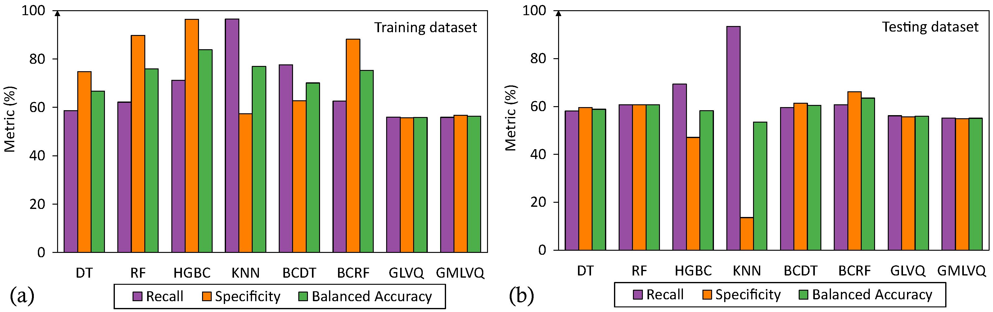
As illustrated in Table A1, the three evaluation metrics are presented for each model with the minimum (min), maximum (max), and mean value (mean) after 50 trials on each training and testing dataset. Figure 2 depicts these metrics separately for (a) the training dataset and (b) the testing dataset. The HGBC attains the highest mean Balanced Accuracy on the training dataset, with KNN and RF following in succession. It is evident that GLVQ and GMLVQ exhibit the lowest values for this metric. On the testing dataset, the KNN exhibits the highest average Recall but also the lowest average Specificity. This observation signifies that the n.p. class is being inadequately classified. This prediction behaviour can be attributed to the imbalance of the dataset, which highlights the problem of overfitting. The application of oversampling was unsuccessful in mitigating this issue. A comparison of the metrics obtained on the training and testing dataset reveals that the majority of models exhibited lower values on the testing dataset. Conversely, GLVQ and GMLVQ represent significant exceptions to this pattern. For these prototype-based models, the Balanced Accuracy on the testing dataset was approximately equivalent to that observed on the training dataset, suggesting a more robust generalisation. It is noteworthy that GLVQ demonstrated a higher level of Recall on the testing dataset than on the training dataset. Notably, this highlights the model’s robustness in identifying the target class. The BCRF has the largest mean Balanced Accuracy, with a well-balanced trade-off between Recall and Specificity. Consequently, it emerged as the best-performing model for predicting WBBT outcomes in this comparison. With regard to the mean values of the performance metrics, this model is closely followed by BCDT and RF.
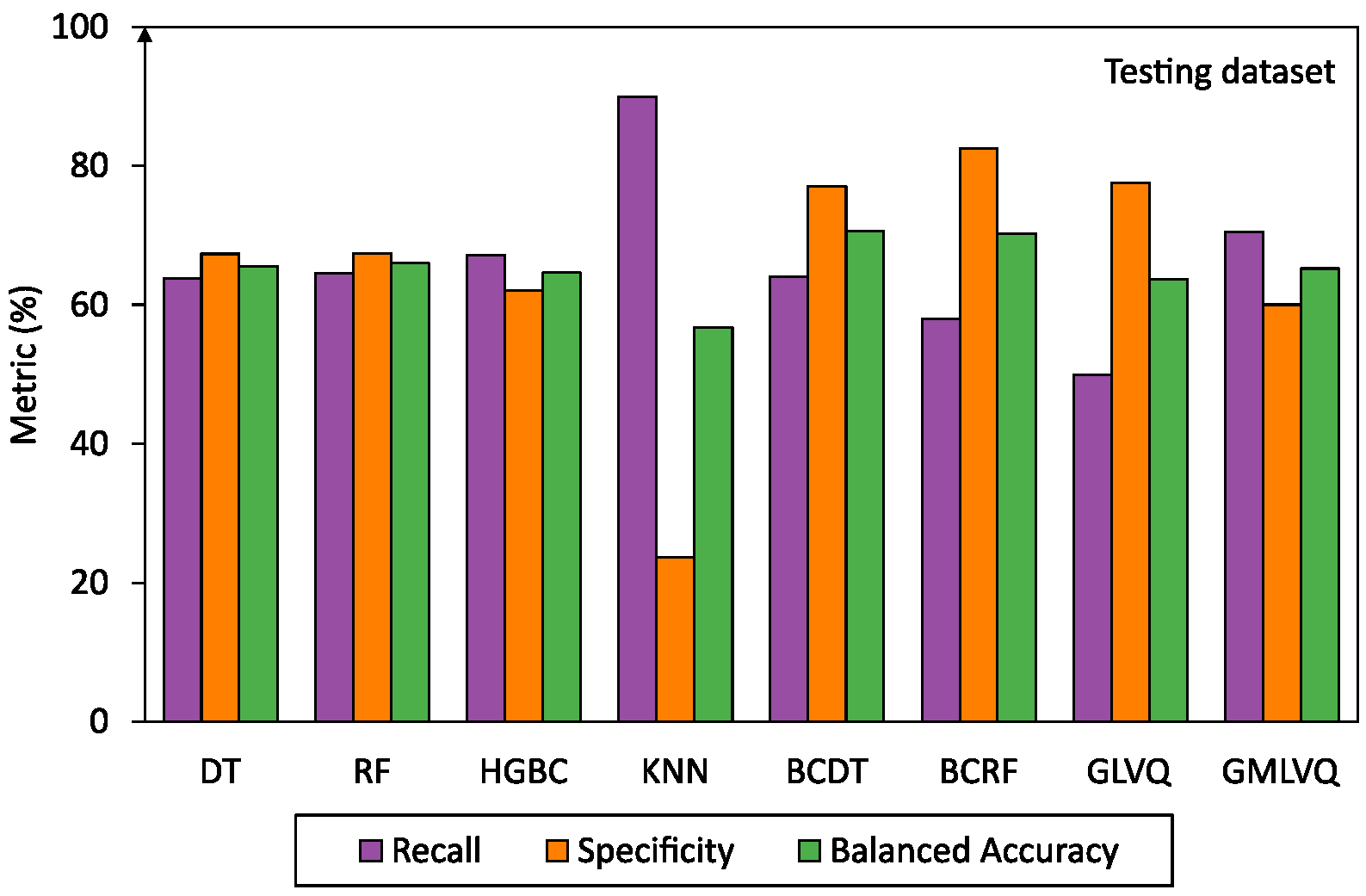
Furthermore, Figure 3 and Table A2 show the metrics of the best single-trials for each model. This demonstrates the strong performance of the BCDT and BCRF ensembles in terms of Balanced Accuracy (70.6%; 70.3%). The latter model demonstrates a higher level of Specificity (SpecificityBCRF = 82.3%; SpecificityBCDT = 77.0%), which facilitates enhanced prediction of the n.p. class by the BCRF. Consequently, this model is assigned the optimal prognostic performance. The weakest predictive ability is also evident when examining the single-trial results for KNN. This model is not capable of reliably predicting the n.p. class, as indicated by its very low Specificity.

3.2. Stability of the Performance

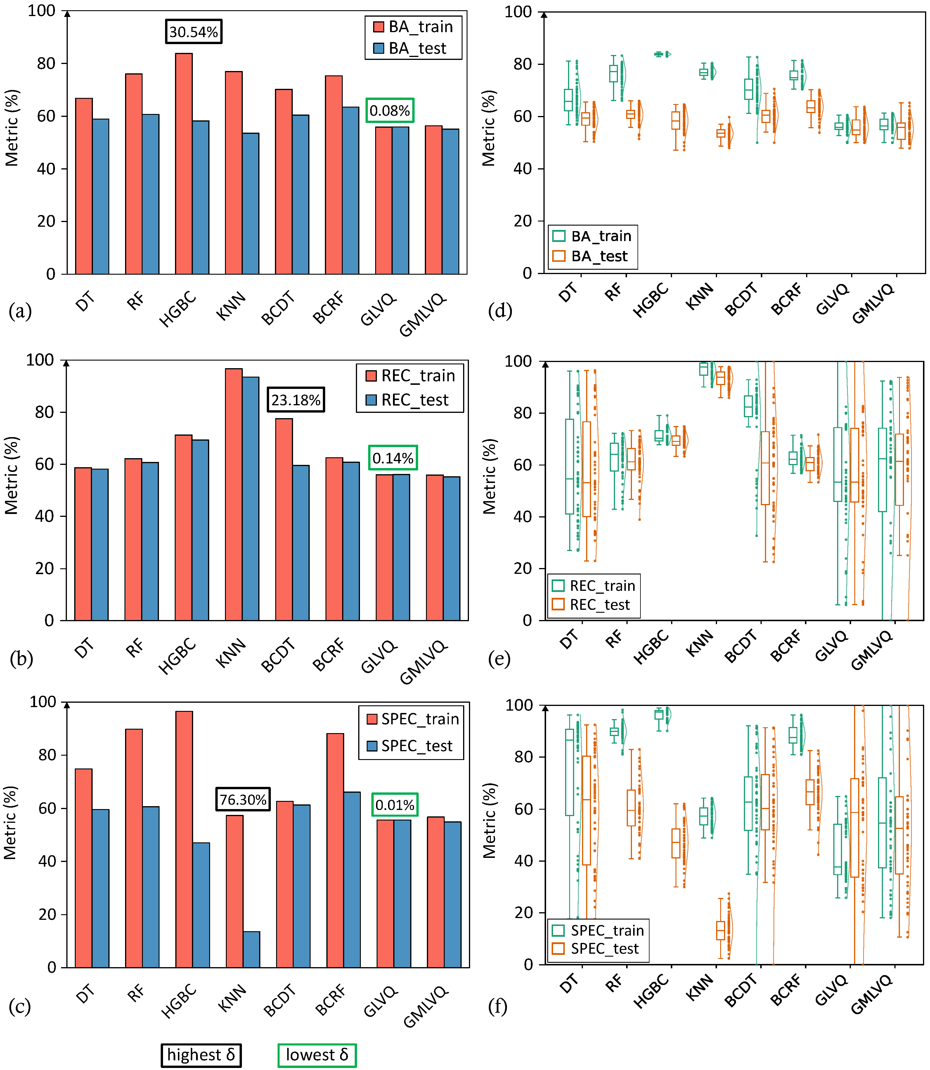
As illustrated in Figure 4, the differences in performance on the training and testing datasets are visualised for the following metrics: (a) Balanced Accuracy, (b) Recall and (c) Specificity. For each model, the values of the stability  δ are listed in the diagram. The strongest stability (lowest δ ) is highlighted in green, while the weakest stability (highest δ ) is represented in black. As illustrated in Table 4, the stability of each model is demonstrated for all three performance evaluation metrics.
The best stability for Balanced Accuracy is achieved by the GLVQ (0.08%), while the most significant disparities between evaluation with training and testing datasets are observed in the HGBC (30.54%) and KNN (30.46%). It is evident that the GLVQ exhibits the smallest δ for the Recall (0.14%). The BCDT shows by far the largest relative deviation at 23.18%. In the context of a model-specific examination of the Specificity, it is observed that there are elevated (KNN, δ = 76.30%) and lowered values for δ (BCDT, δ = 2.23%; GLVQ, δ = 0.01%). The GLVQ and GMLVQ are of particular interest in the context of model stability analysis, as evidenced by their remarkable stability across all three metrics (0.01% to max. 3.17%). Boxplots (Figure 4) represent the distribution of each individual trial for the following metrics: (d) Balanced Accuracy, (e) Recall and (f) Specificity. The model performance for both the training dataset (green) and the testing dataset (orange) was also depicted for this purpose. The smaller the box and whiskers, the narrower the spread of individual model performances, and the more pronounced the peak of the normal distribution. As demonstrated in Figure 4d it is evident that, compared to the training dataset, all models except the GLVQ and GMLVQ exhibit lower Balanced Accuracy on the testing dataset. It can also be seen repeatedly that the model performance for GLVQ and GMLVQ is almost at the same level for these two datasets. It is worthy of note that some individual runs of the BCDT and BCRF achieve significantly higher Balanced Accuracy than any of the other models. As illustrated in Figure 4e, KNN consistently achieves the highest Recall, exhibiting minimal variability across different iterations. HGBC also attains reliably high Recall, while individual trials of the DT and BCDT reach similarly elevated Recall in some cases, but they demonstrate considerable variation, resulting in significantly lower scores in other runs. The GLVQ and GMLVQ exhibit analogous behaviour, with whiskers accounting for almost the entire range of values. The smallest scatter occurs for HGBC, KNN and BCRF when considering Recall. As demonstrated in Figure 4f, DT exhibits substantial scatter in Specificity, obtaining both the highest and also almost the lowest values of this metric in individual trials. However, it should be noted that other models have been observed to show similar performances. A thorough evaluation of the testing dataset reveals that BCDT, GLVQ and GMLVQ demonstrate a broader scatter range, accompanied by a comparatively diminished level of Specificity. It is evident from the evaluation that, when utilising the unknown testing dataset, only the GLVQ is capable of demonstrating an elevated level of Specificity in comparison to the utilisation of known training dataset.

3.3. Computation Time

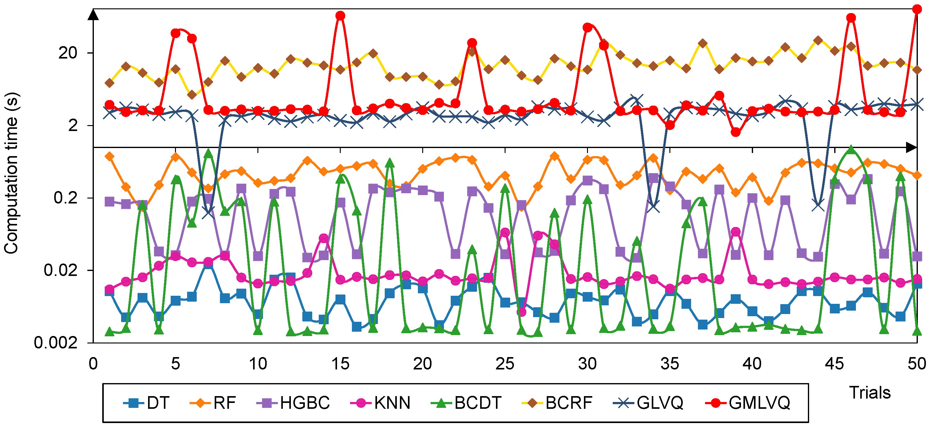
The computation time required by the eight ML models for each trial is depicted in Figure 5, whereas Table A3 presents a statistical summary of the results across 50 trials, including the minimum, maximum, and arithmetic mean values.
It is evident that a considerable disparity exists in the required computation time for the individual models. To address this, the y-axis is scaled logarithmically. DT is characterised by the shortest calculation time, with individual runs almost always completed in under 0.01 s (min = 0.003 s; mean = 0.008 s). KNN has been shown to exhibit a relatively constant computation time, typically below 0.02 s. The BCDT ensemble demonstrates a high degree of variability, with some values ranging from 0.003 s to slightly less than 1 s. A similar observation can be made with HGBC, where values range from 0.003 s to 0.3 s. The computation time of RF is of a medium duration, with minor fluctuations between 0.15 s and 0.76 s. The GLVQ demonstrates a remarkably consistent behaviour within the approximate range of 3 s. With the exception of a few outliers (up to 80.5 s), GMLVQ is in the same time frame, with an average computation time of 10 s. BCRF is evidently the only model that necessitates a higher computation time (mean = 14.33 s), with the majority of single trials requiring between 10 s and 20 s. Despite the substantial disparities, the overall training duration remains relatively short, and the required computation time is of secondary importance given the significant advances in computing resources.

3.4. Evaluation

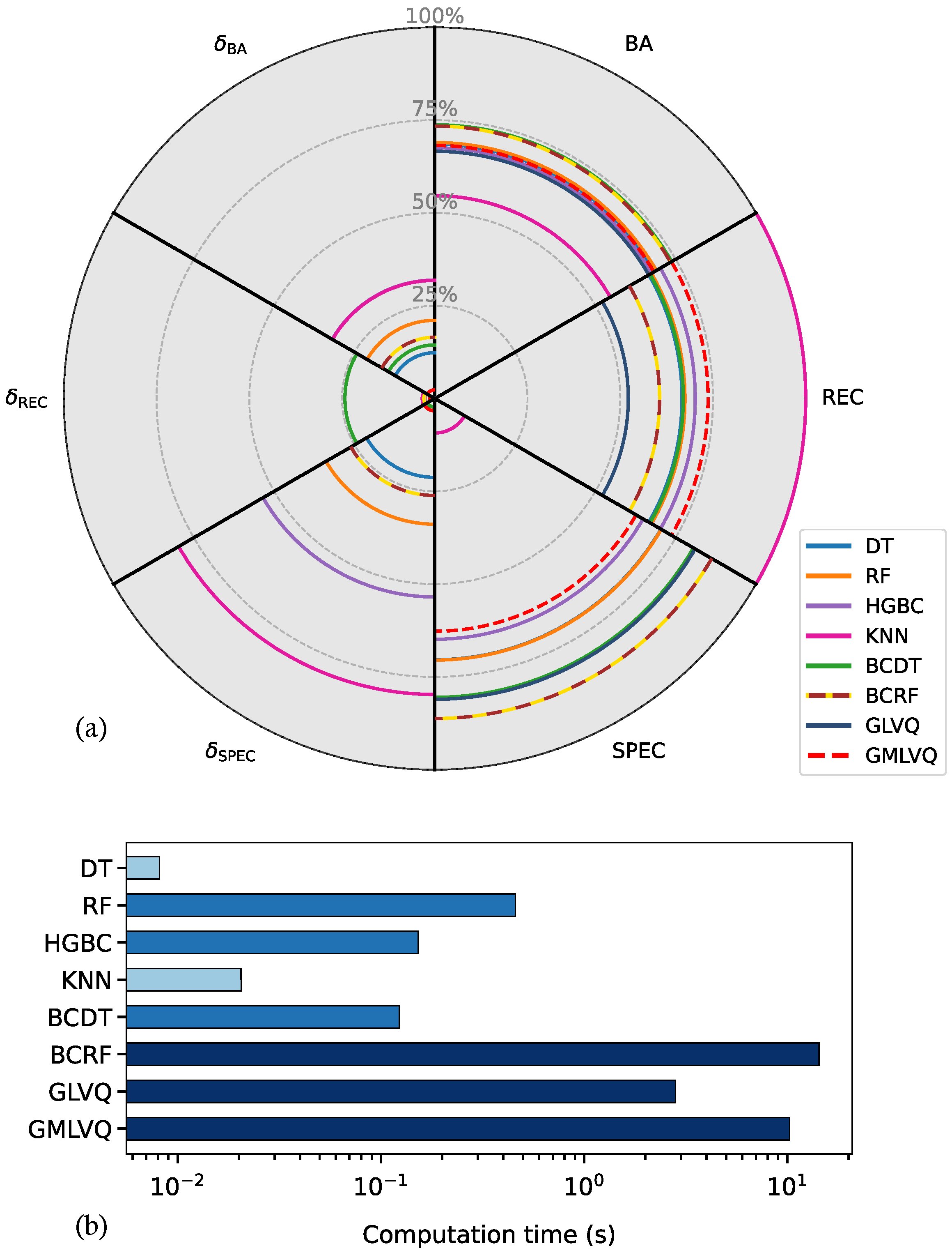
The eight ML models under consideration have been evaluated following 50 trials on both the training and testing datasets. As illustrated in Figure 6a, the three performance metrics of interest—Balanced Accuracy, Recall, and Specificity—are shown from the best single trials of each model, along with the mean stability for each metric. As illustrated in Figure 6b, the average computation time is depicted, thus facilitating the interpretation of the model’s performance whilst accounting for the available computational resources. The colour gradations of the columns illustrate the rough classification of computation times into three categories. DT and KNN: 0.003 s to 0.07 s; RF, HGBC and BCDT: less than 1 s; and BCRF, GLVQ and GMLVQ: an average of 3 s to 15 s. It can be deduced from the evidence presented that BCDT and BCRF achieve the highest Balanced Accuracy in this comparison, with BCRF also requiring the longest computation time. This model further exhibits superior Specificity, rendering it more suitable for the detection of the critical n.p. class. Nevertheless, BCDT and GLVQ also demonstrate favourable results for this metric. The stability of the Balanced Accuracy is only mediocre for BCDT and BCRF. KNN, by contrast, demonstrates an overfitting tendency, characterised by elevated Recall and diminished Specificity. For the p class, GLVQ demonstrates the lowest capability for accurate prediction, as it manifests the smallest Recall. In terms of Specificity, BCRF exhibits moderate stability, whereas BCDT achieves nearly equivalent predictive accuracy for the n.p. class, with a correspondingly very small δ . In the course of the present study, it was found that among all of the evaluated models, GLVQ and GMLVQ exhibited the most stable performance across all three metrics, by far exceeding the stability of the others.

3.5. Feature Importance

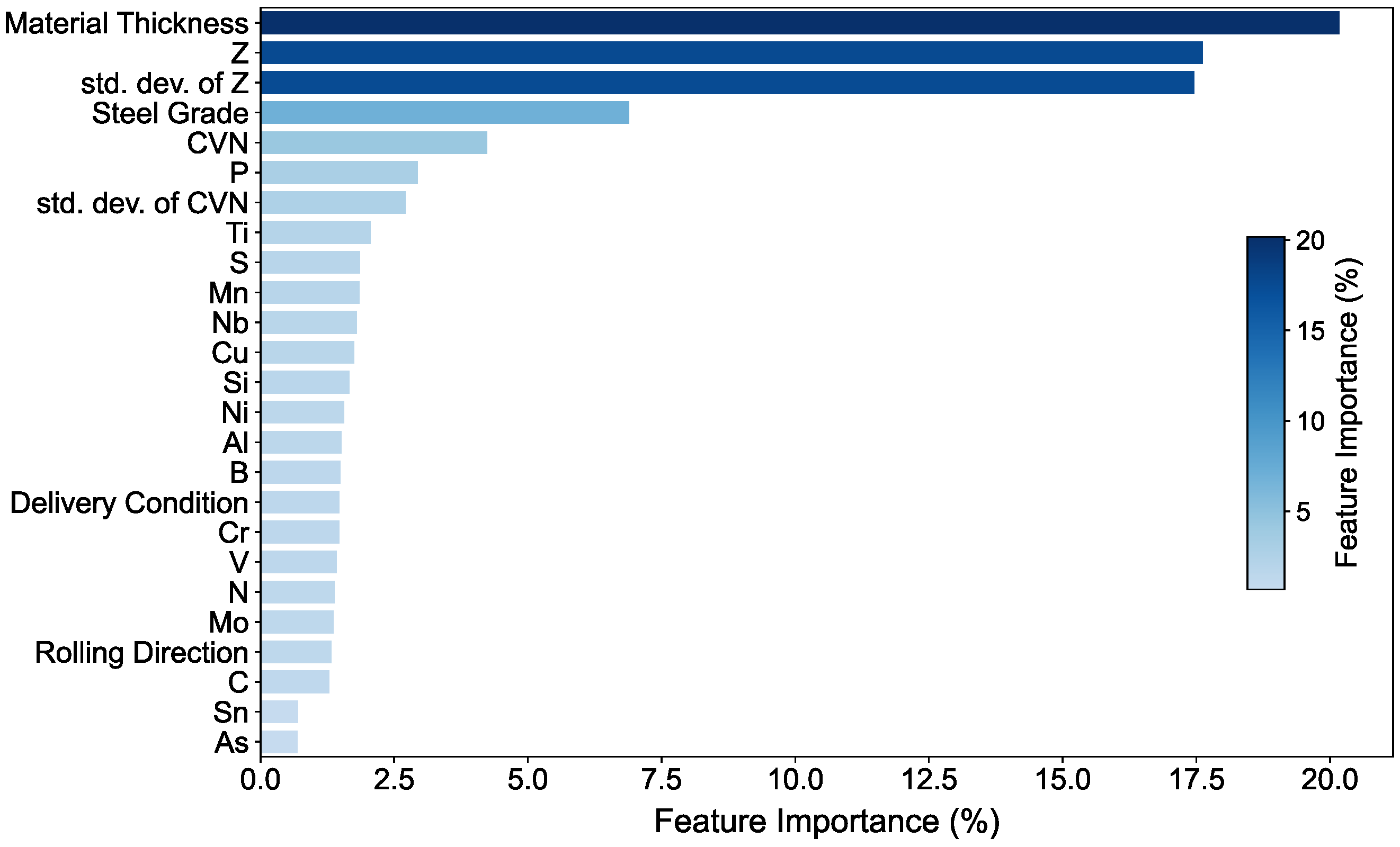
This section presents the feature importance ranking obtained from the best single trial of the top-performing BCRF, as illustrated in Figure 7. The most significant features of the model are the material thickness (20.17%), Z-grade (17.62%), and the standard deviation of the Z-grade (17.46%). Additional relevant features that were identified in the present study include the steel grade (6.89%), CVN (4.24%), content of P (2.94%), and the standard deviation of CVN (2.71%). Conversely, the trace elements Sn (0.70%) and As (0.69%) demonstrate comparatively low feature importance. It was established that several significant features align with previously reported influences on both the outcome of the WBBT and the fracture behaviour of structural steels. In particular, the material thickness has been identified as a significant parameter affecting fracture behaviour in this test by Feldmann et al. [9]. They demonstrated that the test’s toughness requirements increase with increasing material thickness, thereby highlighting its influence on crack initiation and propagation during bending. The significance of toughness-related parameters, particularly CVN, is further substantiated by the research conducted by Sedlacek et al. [10]. In their investigation into replacement criteria for the WBBT, it was demonstrated that higher impact toughness requirements generally correlate with an improved probability of passing the test. However, their findings also highlighted a significant scatter in the data, suggesting that CVN alone may not serve as a definitive predictor. This absence of a clear direct correlation was particularly evident in test plates with borderline toughness properties, leading to the conclusion that the WBBT often functions as an indicator of a binary outcome regarding overall material quality, rather than providing a continuous measure directly relatable to specific impact energy levels. These observations are consistent with the moderate feature importance of CVN (4.24%) and its standard deviation (2.71%) observed in BCRF. It indicates that, while CVN is a contributing factor, it primarily measures energy absorption during dynamic fracture in the longitudinal or transverse direction, which may not fully capture the complex stress state of the WBBT. Notably, the high feature importance assigned to the Z-grade (17.62%) and its standard deviation (17.46%) represents a significant finding that has not been explicitly quantified in previous WBBT literature. While earlier studies acknowledged that the WBBT historically compelled manufacturers to improve overall steel quality, the specific role of through-thickness ductility remained largely qualitative. The present results suggest that Z-grade-related variables, which characterise the material’s resistance to lamellar tearing and its through-thickness integrity, are far more decisive for the test outcome than the traditionally emphasised CVN values.
This is further supported by the identified influence of the phosphorus content (2.94%). According to Bargel and Schulze [32], P is the element that most severely reduces toughness in steel by promoting intergranular fracture and significantly elevating the ductile-to-brittle transition temperature. Furthermore, P exhibits an exceptionally high tendency to segregate due to its low diffusion rate in iron, leading to the formation of marked phosphorus-rich bands (primary banding) during solidification and subsequent forming. These localised inhomogeneities might trigger brittle crack initiation during the WBBT, particularly in thicker plates where such segregation is potentially more prevalent. The comparatively low importance of the trace elements Sn (0.70%) and As (0.69%) should not be interpreted as evidence of a negligible influence on the prediction. Rather, this observation may be attributed to the limited variability of these elements within the dataset. Due to the strong sparsity and narrow value ranges of these features, their statistical contribution to the model may be underestimated. Furthermore, the relatively high feature importance of steel grade (6.89%) should be interpreted with caution. While the BCRF detected patterns where certain steel grades systematically exhibit higher probabilities of n.p. outcomes, this likely reflects the unequal distribution of steel grades within the dataset rather than a direct causal relationship. For individual steel grades represented by only a few samples, the statistical support is limited; thus, the elevated importance of steel grade is attributed to the model’s learning behaviour regarding dataset-specific imbalances.

4. Conclusions

This study evaluates the suitability of eight machine learning classifiers for predicting WBBT outcomes. The aim is to potentially partially omit its execution when the n.p. class can be predicted with sufficiently high probability and accuracy. The investigations focused on the use of DT, RF, HGBC, KNN, BCDT, BCRF, GLVQ and GMLVQ models. An extensive dataset was compiled for the purposes of this study. This comprised approximately 3600 samples and 25 numerical and categorical features. The dataset is characterised by a pronounced class imbalance, with only 6.5% of the samples belonging to the n.p. class. Furthermore, it is marked by considerable sparsity, as certain features are recorded for only 4% to 41% of the samples. All data were collected from material testing carried out at CEWUS. The predictive suitability of the models has been analysed in terms of their performance, which is measured using the metrics of Balanced Accuracy, Recall, Specificity, prediction stability and computation time. Each model was evaluated through 50 independent trials. In each trial, hyperparameter tuning was applied, and the model’s performance was assessed on both training and testing datasets.
  • The models demonstrate disparate performances for both classes (p/n.p.) and in between training and testing datasets. In the majority of cases, the performance on the known training dataset is superior to that on the unknown testing dataset. A very precise prediction of the n.p. class, which corresponds to high Specificity, is crucial for any potential partial substitution of the WBBT.
  • The most stable predictions over all three metrics are achieved by GLVQ ( δ Specificity , GLVQ = 0.01 % up to δ Recall , GLVQ = 0.14 % ) and GMLVQ ( δ Recall , GMLVQ = 1.28 % up to δ Specificity , GMLVQ = 3.17 % ). This is indicative of the excellent generalisation and robustness of these models.
  • The computation time separated the models into three distinct categories: KNN and DT required approximately 0.003 s to 0.07 s for their training. BCDT, HGBC and RF required less than 1 s. GLVQ, BCRF and GMLVQ needed approximately 3 s to 15 s. The latter model exhibited a number of outliers, characterised by elevated computation times (up to 80 s), whereas the BCRF required a consistent time of 10 s to 20 s. It is imperative to acknowledge that the training of a single model is sufficient to enable prediction. This precludes the computation time from being a major performance criterion.
  • BCRF and BCDT exhibited optimal model performance, demonstrating the highest single-trial Balanced Accuracy (70.3%; 70.6%, respectively). BCRF achieved superior Specificity (82.5%) with a Recall of 58%. The n.p. class is detected with a high degree of accuracy. KNN showed the lowest suitability for WBBT outcome prediction. Despite attaining the maximum Recall, this can be ascribed to overfitting, given that the Specificity was considerably diminished.
  • Feature importance analysis for BCRF identified material thickness (20.17%), Z-grade (17.62%), and its standard deviation (17.46%) as the most decisive predictors. The high significance of through-thickness ductility and homogeneity suggests that these parameters are more critical for the WBBT outcome than traditionally emphasised criteria, such as CVN (4.24%).

Author Contributions

Conceptualisation, F.B., U.H., F.H. and K.H.; methodology, F.B.; software, F.B.; validation, F.B. and F.H.; formal analysis, F.B.; investigation, F.B.; resources, F.H. and K.H.; data curation, F.B.; writing—original draft preparation, F.B.; writing—review and editing, K.H.; visualisation, F.B.; supervision, K.H.; project administration, K.H.; funding acquisition, U.H. and K.H. All authors have read and agreed to the published version of the manuscript.

Funding

This research was funded by the European Social Fund (ESF) under grant number 100691067. It constitutes a component of the “ESF-MINT Fachkräfteprogramm ESF Plus 2021 bis 2027” (ESF-STEM Skilled Workers Programme ESF Plus 2021–2027) and is a collaborative initiative between Mittweida University of Applied Sciences and CEWUS GmbH. Further information on the underlying research project of this study is available online [33]: https://www.inw.hs-mittweida.de/webs/wfq/smart-materials/forschung-smart/abvml/, accessed on 8 March 2026. The APC was supported by the Open Access Publication Fund of Mittweida University of Applied Sciences.

Data Availability Statement

The data presented in this study are available on request from the corresponding author. The data are not publicly available due to privacy and legal restrictions related to ongoing research activities.

Acknowledgments

We would like to express our gratitude to CEWUS and in particular to Peter Kaiser and Matthias Hockauf for their invaluable contribution to the comprehensive experimental investigations that have been meticulously compiled in the dataset. We also extend our sincere thanks to Peter Hübner for the fruitful discussions that have greatly enriched this work.

Conflicts of Interest

The authors declare no conflict of interest.

Abbreviations

The following abbreviations are used in this manuscript:
AIArtificial Intelligence
BCDTBagging Classifier with Decision Tree Classifier as base estimator
BABalanced Accuracy
BCRFBagging Classifier with Random Forest Classifier as base estimator
CEWUSChemnitzer Werkstoff und Oberflächentechnik
CVNCharpy V-Notch impact energy
DTDecision Tree Classifier
ESFEuropean Social Fund
FNFalse Negative
FPFalse Positive
GLVQGeneralized Learning Vector Quantizer
GMLVQGeneralized Matrix Learning Vector Quantizer
HAZHeat-Affected Zone
HGBCHistogram-based Gradient Boosting Classifier
KNNk-Nearest Neighbours
MLMachine Learning
n.p. classSamples that did not pass the Welded Bead Bending Test
OESOptical emission spectrometry
p classSamples that passed the Welded Bead Bending Test
RECRecall
RFRandom Forest Classifier
SEPStahl-Eisen-Prüfblatt
SPECSpecificity
std. dev.Standard deviation
TNTrue Negative
TPTrue Positive
WBBTWelded Bead Bending Test
ZZ-Grade from through-thickness tensile test

Appendix A. Performance Metrics

Appendix A.1. 50 Trials

Table A1. Performance metrics after 50 trials on training and testing datasets: Balanced Accuracy (BA), Recall (REC), Specificity (SPEC).
ModelTraining DatasetTesting Dataset
BA (%)REC (%)SPEC (%)BA (%)REC (%)SPEC (%)
DTMin56.9026.9717.6150.4123.0011.11
Max81.2596.2396.2692.4596.4992.45
Mean66.7358.6974.7759.5858.1259.58
RFMin66.1142.9681.0351.4438.9340.91
Max83.3272.2698.2766.0073.3182.98
Mean75.9962.2189.7760.6860.6760.68
HGBCMin82.9567.8690.1047.1863.3330.00
Max84.6679.1298.9964.6474.8862.07
Mean83.8371.2196.4658.2369.3647.11
KNNMin74.3190.1148.9247.9485.952.38
Max80.4699.7864.2959.7997.9227.45
Mean76.9596.5857.3253.5193.4413.58
BCDTMin50.0032.670.0050.0022.580.00
Max82.76100.0092.0570.57100.0091.35
Mean70.0478.0162.0660.4459.5761.31
BCRFMin70.4656.8080.9353.8653.3242.42
Max81.5071.5196.3070.2571.7282.50
Mean75.3762.6088.1363.4660.7966.13
GLVQMin50.006.040.0050.006.160.00
Max60.61100.0099.4963.74100.00100.00
Mean55.8456.0455.6555.8156.0955.53
GMLVQMin50.000.0018.0947.890.0010.64
Max61.3392.38100.0065.2693.82100.00
Mean56.3155.8956.7355.1055.3554.84

Appendix A.2. Best Single Trials

Table A2. Performance metrics of the best single-trials; values of the models achieving the highest Balanced Accuracy (BCDT and BCRF) are highlighted in bold font.
ModelBalanced Accuracy (%)Recall (%)Specificity (%)
DT65.5763.7967.35
RF66.0064.5567.44
HGBC64.6467.2162.07
KNN56.7889.8823.68
BCDT70.5764.1077.05
BCRF70.2558.0082.50
GLVQ63.7449.9377.55
GMLVQ65.2670.5260.00

Appendix B. Computation Time

Table A3. Computation time during training over 50 trials, Min: DT 0.003 s|Max: GMLVQ 80.52 s|lowest Mean: DT 0.008 s.
ModelMin (s)Max (s)Mean (s)
DT0.0030.0240.008
RF0.1490.7590.459
HGBC0.0300.3760.153
KNN0.0050.0680.021
BCDT0.0030.9370.123
BCRF5.3229.7414.33
GLVQ0.1264.4162.875
GMLVQ1.6380.5210.27

References

  1. Salvati, E.; Tognan, A.; Laurenti, L.; Pelegatti, M.; Bona, F.D. A defect-based physics-informed machine learning framework for fatigue finite life prediction in additive manufacturing. Mater. Des. 2022, 222, 111089. [Google Scholar] [CrossRef] [Scilit]
  2. Bruno, F.; Konstantoupoulos, G.; Rossi, E.; Fiore, G.; Charitidis, C.; Sebastiani, M.; Belforte, L.; Palumbo, M. Advanced microstructural characterization in high-strength steels via machine learning-enhanced high-speed nanoindentation and EBSD mapping. Mater. Today Commun. 2024, 39, 109192. [Google Scholar] [CrossRef] [Scilit]
  3. Chang, J.; Li, J.; Ye, J.; Zhang, B.; Chen, J.; Xia, Y.; Lei, J.; Carlson, T.; Loureiro, R.; Korsunsky, A.M.; et al. AI-Enabled Piezoelectric Wearable for Joint Torque Monitoring. Nano-Micro Lett. 2025, 17, 247. [Google Scholar] [CrossRef] [Scilit] [PubMed]
  4. Forschungsgesellschaft für Straßen- und Verkehrswesen (FGSV). Zusätzliche Technische Vertragsbedingungen und Richtlinien für Ingenieurbauten ZTV-ING; Technical report; Bundesministerium für Digitales und Verkehr (BMDV): Berlin, Germany, 2023. [Google Scholar]
  5. DBS 918 002-02; Technische Lieferbedingungen: Warmgewalzte Erzeugnisse aus Baustählen für den Eisenbahnbrückenbau. Technical report; Deutsche Bahn AG: Berlin, Germany, 2006.
  6. SEP 1390; Aufschweißbiegeversuch. Technical report; Verein Deutscher Eisenhüttenleute (VDEh): Düsseldorf, Germany, 1996.
  7. Stranghöner, N. Der Aufschweißbiegeversuch oder: Nichts ist beständiger als ein Provisorium. Stahlbau 2009, 78, 815–821. [Google Scholar] [CrossRef] [Scilit]
  8. DIN EN 1993-1-1:2025-04; Eurocode 3: Design of Steel Structures—Part 1-1: General Rules and Rules for Buildings. Technical report; Deutsches Institut für Normung (DIN): Berlin, Germany, 2025.
  9. Feldmann, M.; Citarelli, S.; Münstermann, S.; Könemann, M. AUBI-äquivalente Anforderungen an die Zähigkeitshochlage aus Versuchen und Schädigungssimulationen. Stahlbau 2020, 89, 1016–1026. [Google Scholar] [CrossRef] [Scilit]
  10. Sedlacek, G.; Höhler, S.; Dahl, W.; Kühn, B.; Langenberg, P.; Finger, M.; Floßdorf, F.J.; Schröter, F.; Hocké, A. Ersatz des Aufschweißbiegeversuchs durch äquivalente Stahlgütewahl. Stahlbau 2005, 74, 539–546. [Google Scholar] [CrossRef] [Scilit]
  11. DIN EN ISO 2560; Welding Consumables—Covered Electrodes for Manual Metal Arc Welding of Non-Alloy and Fine Grain Steels—Classification. Technical report; Deutsches Institut für Normung (DIN): Berlin, Germany, 2021.
  12. Backofen, F.; Hähnel, U.; Hahn, F.; Hockauf, M.; Kaiser, P.; Hockauf, K. Prediction of the Outcome of a Welded Bead Bending Test (WBBT) using Machine Learning (ML). In Proceedings of the 43. Vortrags- und Diskussionstagung Werkstoffprüfung 2025; Zimmermann, M., Ed.; Deutsche Gesellschaft für Materialkunde e.V. (DGM): Nordrhein-Westfalen, Germany, 2025; pp. 86–91. [Google Scholar]
  13. Breiman, L.; Friedman, J.H.; Olshen, R.A.; Review, C.J.S.; Gordon, A.D. Classification and Regression Trees; Wadsworth International Group: New York, NY, USA, 1984; Volume 40, p. 874. [Google Scholar]
  14. Quinlan, J.R. Induction of Decision Trees. Mach. Learn. 1986, 1, 81–106. [Google Scholar] [CrossRef] [Scilit]
  15. Cover, T.M.; Hart, P.E. Nearest Neighbor Pattern Classification. IEEE Trans. Inf. Theory 1967, 13, 21–27. [Google Scholar] [CrossRef] [Scilit]
  16. Breiman, L. Bagging Predictors. Mach. Learn. 1996, 24, 123–140. [Google Scholar] [CrossRef] [Scilit]
  17. Breiman, L. Random Forests. Mach. Learn. 2001, 45, 5–32. [Google Scholar] [CrossRef] [Scilit]
  18. Ke, G.; Meng, Q.; Finley, T.; Wang, T.; Chen, W.; Ma, W.; Ye, Q.; Liu, T.Y. LightGBM: A Highly Efficient Gradient Boosting Decision Tree. In Proceedings of the Advances in Neural Information Processing Systems 30; Curran Associates, Inc.: Red Hook, NY, USA, 2017; pp. 3146–3154. Available online: https://dl.acm.org/doi/10.5555/3294996.3295074 (accessed on 7 April 2026).
  19. Theerthagiri, P. Liver disease classification using histogram-based gradient boosting classification tree with feature selection algorithm. Biomed. Signal Process. Control 2025, 100, 107102. [Google Scholar] [CrossRef] [Scilit]
  20. Sato, A.; Yamada, K. Generalized Learning Vector Quantization. In Proceedings of the Advances in Neural Information Processing Systems; MIT Press: Cambridge, MA, USA, 1996; pp. 423–429. [Google Scholar]
  21. Schneider, P.; Schleif, F.M.; Villmann, T.; Biehl, M. Generalized Matrix Learning Vector Quantizer for the Analysis of Spectral Data. In Proceedings of the 16th European Symposium on Artificial Neural Networks (ESANN 2008), Bruges, Belgium, 23–25 April 2008; D-Side Publications: Bruges, Belgium, 2008; pp. 451–456. [Google Scholar]
  22. Rojek, I.; Jasiulewicz-Kaczmarek, M.; Piechowski, M.; Mikołajewski, D. The use of decision trees to identify the causes of failures in a medical enterprise—A case study. In Proceedings of the IFAC-PapersOnLine; Elsevier B.V.: Amsterdam, The Netherlands, 2024; Volume 58, pp. 133–138. [Google Scholar] [CrossRef] [Scilit]
  23. Tang, Y.; Chang, Y.; Li, K. Applications of K-nearest neighbor algorithm in intelligent diagnosis of wind turbine blades damage. Renew. Energy 2023, 212, 855–864. [Google Scholar] [CrossRef] [Scilit]
  24. Tharwat, A.; Gaber, T.; Awad, Y.M.; Dey, N.; Hassanien, A.E. Plants identification using feature fusion technique and bagging classifier. In Proceedings of the Advances in Intelligent Systems and Computing; Springer: Berlin/Heidelberg, Germany, 2016; Volume 407, pp. 461–471. [Google Scholar] [CrossRef] [Scilit]
  25. Patel, R.K.; Giri, V. Feature selection and classification of mechanical fault of an induction motor using random forest classifier. Perspect. Sci. 2016, 8, 334–337. [Google Scholar] [CrossRef] [Scilit]
  26. Deb, C.; Nachiappan, M.R.; Elangovan, M.; Sugumaran, V. Fault Diagnosis of a Single Point Cutting Tool using Statistical Features by Random Forest Classifier. Indian J. Sci. Technol. 2016, 9, 1–8. [Google Scholar] [CrossRef] [Scilit]
  27. Saifudin, A.; Nabillah, U.U.; Yulianti; Desyani, T. Bagging Technique to Reduce Misclassification in Coronary Heart Disease Prediction Based on Random Forest. In Proceedings of the Journal of Physics: Conference Series; Institute of Physics Publishing: Bristol, UK, 2020; Volume 1477. [Google Scholar] [CrossRef] [Scilit]
  28. S., M.E.; Fajar, M.; T., M.I.; Jatmiko, W. FNGLVQ FPGA Design for Sleep Stages Classification based on Electrocardiogram Signal. In Proceedings of the IEEE International Conference on Systems, Man, and Cybernetics; IEEE: New York, NY, USA, 2012. [Google Scholar]
  29. van Veen, R.; Gurvits, V.; Kogan, R.V.; Meles, S.K.; de Vries, G.J.; Renken, R.J.; Rodriguez-Oroz, M.C.; Rodriguez-Rojas, R.; Arnaldi, D.; Raffa, S.; et al. An application of generalized matrix learning vector quantization in neuroimaging. Comput. Methods Programs Biomed. 2020, 197, 105708. [Google Scholar] [CrossRef] [Scilit] [PubMed]
  30. Fan, J.; Yue, W.; Wu, L.; Zhang, F.; Cai, H.; Wang, X.; Lu, X.; Xiang, Y. Evaluation of SVM, ELM and four tree-based ensemble models for predicting daily reference evapotranspiration using limited meteorological data in different climates of China. Agric. For. Meteorol. 2018, 263, 225–241. [Google Scholar] [CrossRef] [Scilit]
  31. Li, X.; Luan, F.; Wu, Y. A comparative assessment of six machine learning models for prediction of bending force in hot strip rolling process. Metals 2020, 10, 685. [Google Scholar] [CrossRef] [Scilit]
  32. Bargel, H.J.; Schulze, G. Werkstoffkunde, 11th ed.; Springer: Berlin/Heidelberg, Germany, 2012. [Google Scholar] [CrossRef] [Scilit]
  33. ABVML Project—Smart Materials Research. Available online: https://www.inw.hs-mittweida.de/webs/wfq/smart-materials/forschung-smart/abvml/ (accessed on 9 April 2025).
Figure 1. (a) Setup of the WBBT (schematic), (b) p sample, (c) n.p. sample, (d) invalid sample, (e) detail of (b), (f) detail of (d).
Metals 16 00418 g001
Figure 2. Mean values of the performance metrics for (a) training dataset and (b) testing dataset after 50 trials.
Metals 16 00418 g002
Figure 3. Performance metrics of the best single trials.
Metals 16 00418 g003
Figure 4. Stability  δ of the models as an indicator of the differences in performance metrics achieved when utilising the training and testing datasets: Numerical values displayed = δ ; (a) Balanced Accuracy (BA), (b) Recall (REC), (c) Specificity (SPEC); distribution of metrics after 50 trials on training and testing datasets using boxplots: (d) Balanced Accuracy (BA), (e) Recall (REC), (f) Specificity (SPEC).
Metals 16 00418 g004
Figure 5. Computation time of the eight ML models displayed over all 50 trials of training.
Metals 16 00418 g005
Figure 6. Performance evaluation of the eight ML models after 50 trials on training and testing datasets using best single-trial values of (a) Balanced Accuracy (BA), Recall (REC), Specificity (SPEC) and mean stability  δ ; (b) mean computation time: highest Balanced Accuracy and Specificity: BCRF|highest stability: GLVQ and GMLVQ|longest computation time: BCRF, GLVQ, GMLVQ.
Metals 16 00418 g006
Figure 7. Feature importance of the best-performing single-trial of BCRF. Most significant features: material thickness, Z-grade and std. dev. of the Z-grade.
Metals 16 00418 g007
Table 1. Imbalanced composition of the dataset.
Number of Samplesp Class (%)n.p. Class (%)
359993.56.5
Table 2. Features and their incomplete presence in the dataset.
Type of FeatureFeatureSamples with This Feature (%)
Numericalmaterial thickness (mm)100.0
Z (%)40.9
std. dev. of Z (%)40.8
CVN (J)19.8
std. dev. of CVN (J)19.8
Sn [wt%]4.0
B [wt%]8.6
C [wt%]18.9
Mn [wt%]18.9
Si [wt%]18.9
S [wt%]18.7
P [wt%]18.9
Cr [wt%]18.8
Ni [wt%]18.6
Cu [wt%]18.6
As [wt%]4.1
Ti [wt%]17.1
N [wt%]18.2
Al [wt%]18.7
Mo [wt%]15.6
V [wt%]17.0
Nb [wt%]17.5
Categoricalsteel grade/material100.0
delivery condition99.7
rolling direction100.0
Table 3. Overview of the implemented models for classification.
ModelArchitectureRemarksSuccessful Applications
DT [13,14]Tree structure via recursive feature partitioning; splits by metrics (e.g., information gain); stop by depth/size; pruning prevents overfittingGood interpretability; risk of overfitting; flexible (classification and regression)Fault cause analysis in manufacturing [22]
KNN [15]Instance-based, non-parametric; prediction by majority vote of the k nearest neighbours; lazy learningSuitable for multiclass classification; long computation times for large datasetsDiagnosis of wind turbine blade damage [23]
BCDT [16]Ensemble of DTs; each tree trained on a bootstrap sample; final prediction by majority voteReduces variance and overfitting; improves stability and accuracy; insensitive to individual outliersPlant identification [24]
RF [17]Ensemble of DTs using bagging and random feature selection; final prediction by majority voteReduces variance and overfitting; delivers stable and robust predictionsSteel microstructure characterisation [2]; fault classification for induction motors [25]; cutting tool fault diagnosis [26]
BCRF [16]Ensemble of RF base models; each RF trained on a bootstrap sample; final prediction by majority voteReduces variance, stabilises predictions, increases accuracyCoronary heart disease prediction [27]; prediction of WBBT [12]
HGBC [18]Gradient boosting: sequential weak learners (e.g., DTs); histogram-based binning for faster splitsSuitable for large, mixed datasets; high accuracy; efficient and fast trainingLiver disease prediction [19]
GLVQ [20]Prototype-based classification; classes represented by prototypes; assignment by relative distanceRobust performance; clear separation between class prototypesSleep stage classification from ECG [28]
GMLVQ [21]GLVQ extension with learned distance metric; input assigned to nearest prototypeImproved performance; handles high-dimensional data; interpretable; weighs relevant featuresNeurodegenerative disease classification [29]
Table 4. Stability δ of the evaluated models; best values are highlighted in bold font.
Model δ Balanced Accuracy (%) δ Recall (%) δ Specificity (%)
DT11.810.9620.32
RF20.152.4832.40
HGBC30.542.5951.16
KNN30.463.2576.30
BCDT13.8123.182.23
BCRF15.802.8225.00
GLVQ0.080.140.01
GMLVQ2.241.283.17
Disclaimer/Publisher’s Note: The statements, opinions and data contained in all publications are solely those of the individual author(s) and contributor(s) and not of MDPI and/or the editor(s). MDPI and/or the editor(s) disclaim responsibility for any injury to people or property resulting from any ideas, methods, instructions or products referred to in the content.