Article

Coupling Approach of Crystal Plasticity and Machine Learning in Predicting Forming Limit Diagram of AA7075-T6 at Various Temperatures and Strain Rates

1
Department of Materials Engineering and Convergence Technology, Gyeongsang National University, Jinju 52828, Republic of Korea
2
Materials Processing Research Division, Korea Institute of Materials Science, Changwon 51508, Republic of Korea
*
Authors to whom correspondence should be addressed.
Metals 2026, 16(1), 21; https://doi.org/10.3390/met16010021
Submission received: 3 November 2025 / Revised: 23 December 2025 / Accepted: 23 December 2025 / Published: 25 December 2025
(This article belongs to the Section Crystallography and Applications of Metallic Materials)

Abstract

This study proposes a data-driven framework for predicting forming limit diagrams (FLDs) of AA7075-T6 aluminum sheets under various temperatures and strain rates. To overcome the limitations of costly and time-consuming experiments, a hybrid dataset combining experimental results and virtual data from rate-dependent crystal plasticity finite element (CPFE) simulations coupled with the Marciniak–Kuczyński (M–K) model was developed. Several machine learning (ML) models—including linear regression (LR), random forest regression (RFR), support vector regression (SVR), Gaussian process regression (GPR), and multilayer perceptron (MLP)—were trained to predict FLDs. The nonlinear dependence of the FLD on temperature and strain rate was accurately captured by the ML models, with nonlinear algorithms demonstrating notably improved predictive performance. The proposed approach offers an efficient, accurate, and cost-effective method for FLD prediction and supports data-driven process design in lightweight alloy forming.

1. Introduction

The aluminum alloy AA7075 has been widely utilized in aerospace, automotive, and lightweight structural applications owing to its high specific strength and excellent stiffness-to-weight ratio [1,2,3]. However, despite its superior mechanical strength, AA7075-T6 sheets exhibit inherently low ductility and poor formability at room temperature. This limitation results in severe cracking during cold forming, making it difficult to manufacture complex-shaped components. Furthermore, the alloy shows poor bendability and a pronounced susceptibility to strain localization under room-temperature forming conditions, which restricts its application to structural components requiring high formability.
To overcome these intrinsic drawbacks, temperature-assisted forming technologies have emerged as effective solutions. Numerous studies have reported a significant improvement in both the elongation and formability of AA7075-T6 sheets when warm forming is conducted [2,4,5,6]. In addition to warm forming, which performs forming under isothermal conditions, extensive research has also been conducted on the W-temper forming technique, which enhances ductility through pre-heat treatment and enables forming at room temperature. Nonetheless, the optimization of warm forming conditions requires a comprehensive understanding of the material’s formability under various combinations of temperature and strain rate, which are known to strongly influence the deformation mechanisms and fracture behavior of aluminum alloys [7,8,9]. In this regard, the forming limit diagram (FLD) serves as a fundamental design tool that defines the onset of localized necking under different strain paths, enabling the prediction and prevention of failure during sheet forming processes [10,11]. However, constructing comprehensive FLDs over a wide range of process parameters through physical experiments, such as so-called Nakajima or Marciniak tests, is both time-consuming and costly. In particular, performing experiments under various combinations of temperature and strain rate conditions is highly inefficient in terms of both time and cost. Each test requires meticulous thermal control, repeated trials for statistical reliability, and high-precision optical strain measurement systems, making it impractical to fully map the forming limits under all relevant conditions.
The integration of physics-based simulation and machine learning (ML) [12,13,14,15] has recently gained increasing attention as a promising approach to efficiently predict forming behavior across a wide range of process windows. ML models, once trained on sufficient and representative data, can accurately capture complex nonlinear relationships between process variables and material responses without requiring repeated experiments. Several studies have demonstrated that ML algorithms can successfully predict forming parameters, including flow stress, fracture strain, and forming limits [12,13,14,15,16,17]. Chheda et al. (2019) developed a two-stage ML framework combining support vector and gradient-boost regression to predict FLDs of aluminum alloys [17]. Jaremenko et al. (2019) employed a convolutional neural network to automatically determine probabilistic FLDs [16]. Li et al. (2023) constructed a neural-network-based hardening and ductile-fracture model that captured the coupled effects of stress triaxiality, Lode parameter, strain rate, and temperature on failure [13]. Yatkın and Kõrgesaar (2024) compared several ML algorithms trained on synthetic data from conventional Marciniak–Kuczyński (M–K) predictions assuming isotropic behavior of the material [12]. Finally, Samad et al. (2025) applied supervised ML models to estimate FLDs and fracture FLDs of various sheet metals [14]. Together, these works highlight the evolution of ML-based formability prediction from regression-driven modeling toward deep learning frameworks capable of generalizing across alloys and forming conditions.
Nevertheless, one major obstacle remains in the previously reported approaches, that is, the scarcity of high-quality data necessary to train reliable ML models. In particular, experimental datasets for AA7075-T6 at elevated temperatures and varying strain rates are limited due to the difficulties associated with high-temperature mechanical testing and formability measurements. In fact, although Li et al. (2023) conducted an in-plane fracture test on AA7075-T6 sheets to predict fracture loci under various temperatures and strain rates, studies involving FLD determination using out-of-plane Nakajima tests and subsequent ML training have been performed only at a single temperature and strain rate [13]. In addition, previous studies utilized virtual datasets obtained from the M–K model for the ML training. However, the M–K model adopted in those works followed a conventional formulation that did not account for complex deformation behaviors of materials, such as plastic anisotropy and strain rate sensitivity. In particular, the AA7075-T6 alloy is known to exhibit pronounced plastic anisotropy [18] and strong strain rate sensitivity [10] at elevated temperatures. Therefore, when generating the virtual data for ML training through M–K model simulations, it is essential to incorporate these complex deformation characteristics to ensure realistic and physically consistent predictions. An alternative strategy is therefore required to generate extensive datasets that reflect realistic deformation behavior under diverse forming conditions.
An alternative and promising approach is to employ crystal plasticity finite element (CPFE) simulations coupled with the M–K model to generate synthetic FLD data [19,20,21,22]. The CPFE model, grounded in dislocation density-based constitutive laws, enables microstructurally informed predictions of anisotropic plastic flow and temperature-dependent hardening [23], while the M–K model accounts for the initiation of localized necking caused by geometric imperfections. Furthermore, the rate-dependent crystal plasticity model inherently accounts for strain-rate sensitivity, enabling a more realistic description of strain rate sensitive deformation behavior [24,25,26]. Finally, when combined, this hybrid M–K model can predict forming limits over a wide range of temperatures and strain rates with high physical fidelity. Such hybrid modeling serves as a powerful tool to augment the dataset used for ML training; therefore, it can effectively fill the gap between limited laboratory results and the large dataset requirements of ML algorithms [27].
Building upon these insights, the present study proposes an integrated framework that couples the hybrid M–K model with machine learning to predict the FLDs of AA7075-T6 sheets across a broad spectrum of temperatures and strain rates. First, the dislocation density-based CPFE model was calibrated using tensile test results obtained at various temperatures and strain rates, and the corresponding constitutive parameters were implemented into the hybrid M–K model to virtually predict the FLDs. The experimentally measured and model-predicted FLDs were then combined to construct a comprehensive dataset that encompasses both physical and virtual information. Various ML algorithms, namely, linear regression (LR), random forest regression (RFR), support vector regression (SVR), Gaussian process regression (GPR), and multilayer perceptron (MLP), were trained and optimized to predict the major strain at necking (ε1) as a function of temperature, strain rate, and strain ratio. The predictive accuracy of these ML models was systematically evaluated. Finally, the evaluation demonstrated that the proposed approach not only accurately reproduces the experimentally observed temperature- and strain-rate-dependent trends in FLD but also substantially reduces the need for extensive physical experimental testing.
In summary, this work presents a novel data-driven hybrid modeling strategy that integrates CPFE, the M–K framework, and ML to efficiently and accurately predict the FLDs of AA7075-T6 aluminum alloy under diverse thermo-mechanical conditions. The proposed methodology provides a cost-effective pathway for designing temperature-assisted forming processes and can be extended to other lightweight alloys where experimental data are limited.

2. Materials and Methods

This section outlines the experimental procedures employed in this study, including the materials used and the mechanical testing procedures, namely uniaxial tensile testing and forming limit determination.

2.1. Materials

In this study, AA7075-T6 aluminum alloy sheets with a nominal thickness of 1 mm, supplied by Kaiser Aluminum Corporation, were employed (Foothill Ranch, CA, USA). The chemical composition of the alloy is summarized in Table 1. The initial microstructure of the as-received sheet, examined by EBSD, is shown in Figure 1. The orientation distribution indicates a recrystallized texture, dominated by the R {124}⟨211⟩ component, with minor contributions from the P {011}⟨122⟩, Goss {011}⟨100⟩, and Cube {001}⟨100⟩ components. The average grain size is approximately 62.5 μm.

2.2. Uniaxial Tensile Test

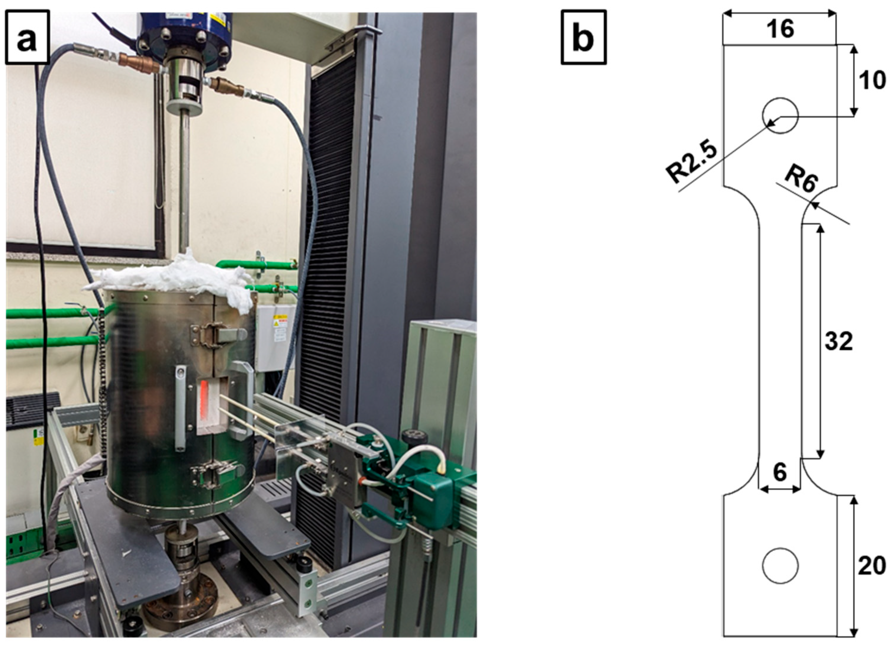
Uniaxial tensile experiments were performed to evaluate the tensile behavior of the aluminum sheet under different temperatures and strain rates. The tests were conducted using a universal testing machine equipped with a furnace, as shown in Figure 2a. The furnace was capable of maintaining the testing temperature within ±5 °C of the target value, ensuring uniform heating of the specimen during deformation. The specimen geometry and dimensions used for uniaxial tensile testing are presented in Figure 2b. The tensile specimens were machined from AA7075-T6 sheets along the rolling direction (RD), with a gauge length of 25 mm and a width of 6 mm. Prior to testing, each specimen was held at the designated temperature for 10 min to achieve thermal equilibrium. The cross-head speed was controlled to maintain a nominal strain rate, and the tests were conducted at different strain rates of 0.001 and 0.1/s. Tests were conducted at various temperatures, i.e., 25, 200, 250, 300, 400, and 470 °C. The strain was measured using a high-temperature ceramic extensometer with a 25 mm gauge length. All tests were repeated at least three times to confirm reproducibility.

2.3. Forming Limit Determination

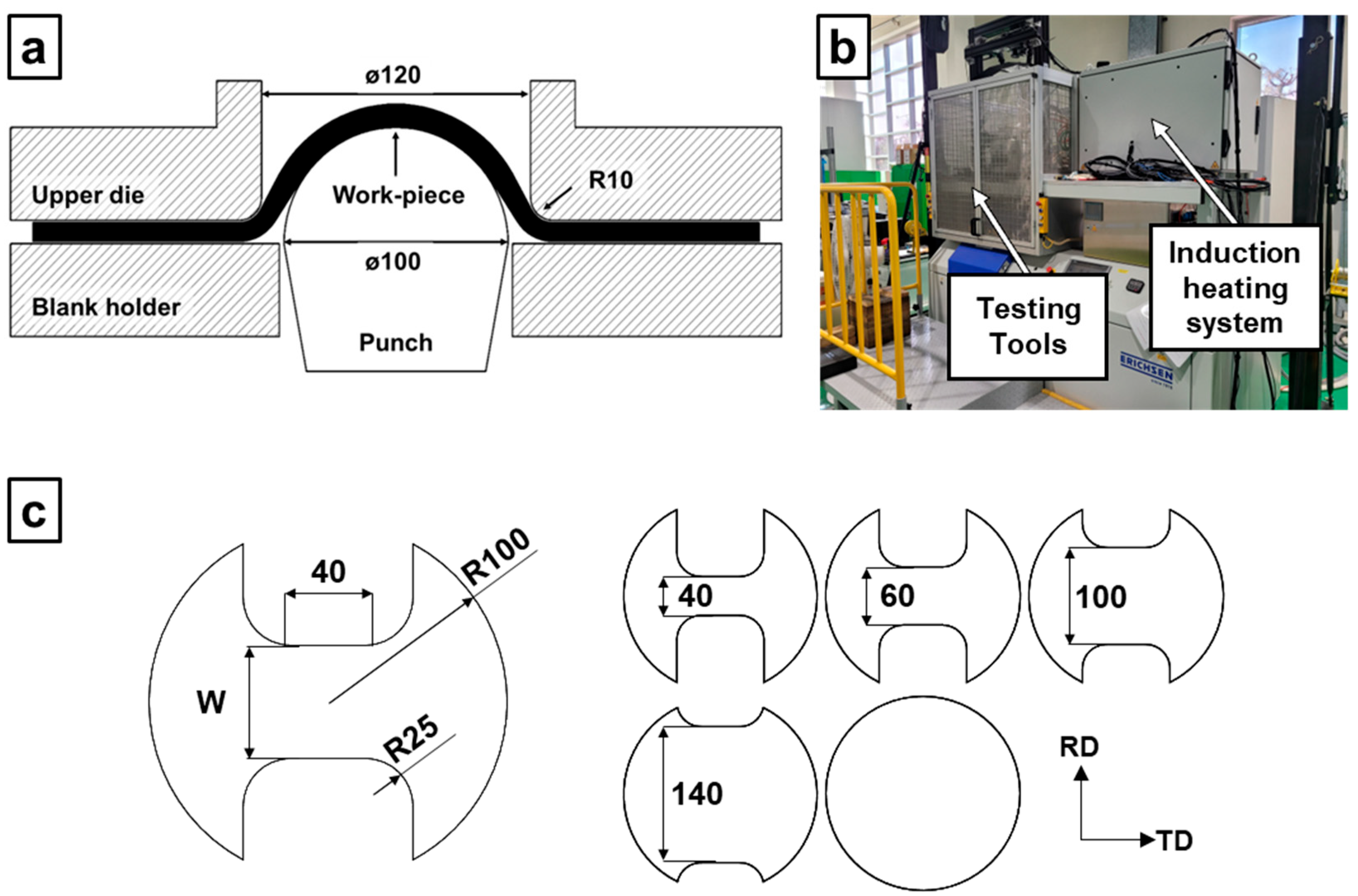
In this study, the FLD was obtained through Nakajima-type dome stretching experiments conducted in accordance with ISO 12004-2 [28], which defines a standardized methodology for assessing the formability of sheet materials. A schematic illustration of the experimental configuration based on this standard is presented in Figure 3a. The testing apparatus utilized a hemispherical punch with a diameter of 100 mm. A constant blank-holding force of 200 kN was maintained throughout the tests, while the punch was driven upward at two different velocities, 0.17 mm/s and 1.7 mm/s, corresponding to average strain rates of approximately 0.002/s and 0.03/s, respectively. The specimen geometries recommended by ISO 12004-2 are shown in Figure 3c. By altering the width of the remaining blank, various strain paths were generated, enabling the construction of a complete FLD.
The forming limit tests were carried out using a universal sheet metal testing machine (Model 142-60, Erichsen GmbH, Hemer, Germany) equipped with an induction heating system, as shown in Figure 3c. Experiments were conducted at three different temperatures of 200, 300, and 400 °C. To minimize friction during deformation, boron nitride was applied as a lubricant between the punch and specimen surface. A square grid pattern with a diameter of 1 mm was etched on the specimen surface prior to testing to enable strain measurement. After testing, the deformed specimens were analyzed ex situ using the ARGUS 3D (https://www.zeiss.com/metrology/en/systems/optical-3d/3d-testing/argus.html, accessed on 22 December 2025) optical strain measurement system to obtain the strain distribution. From the measured strain fields, major and minor strains were extracted along a line perpendicular to the fracture zone, and the forming limit strains were determined by fitting a reverse second-order polynomial to the data. Each experimental condition was repeated three times to ensure the reproducibility of the results.

3. Crystal Plasticity Finite Element Model

This section describes the fundamental theory of the CPFE model developed to simulate the mechanical behavior of the AA7075-T6 sheet under various temperatures and strain rates. In addition, the hybrid M–K model, which integrates the CPFE and the M–K models, is introduced to predict the FLD.

3.1. Dislocation Density-Based Crystal Plasticity Model

In the study, a dislocation density-based crystal plasticity model is employed. Within this framework, the total deformation gradient tensor F is multiplicatively decomposed into elastic and plastic components:
F = F e F p
Here, F e represents the elastic distortion associated with rigid-body rotation, whereas F p describes the plastic deformation arising from crystallographic slip deformation.
The second Piola–Kirchhoff stress tensor is obtained as follows:
S e = C e : E e
where the elastic strain measure E e is defined as follows:
E e = 1 2 F e T F e I
Here, C e is the fourth-order stiffness tensor associated with the given crystal orientation, while I represents the identity tensor. From Equation (2), the Cauchy stress σ is evaluated as follows:
σ = 1 det F e F e S e F e T
In crystal plasticity theory, the plastic velocity gradient L p is expressed as the sum of plastic shear rates γ ˙ α over all active slip systems α :
L p = F ˙ p F p 1 = α = 1 N γ ˙ α s 0 α n 0 α
Here, s 0 α and n 0 α denote the slip direction and slip plane normal of the α -th slip system, respectively, and N is the total number of slip systems.
Based on the rate-dependent crystal plasticity formulation, the plastic shear rate γ ˙ α is determined using a power-law-type relation between the resolved shear stress τ α and the slip resistance g α :
γ ˙ α = γ ˙ 0 τ α g α 1 / m sgn τ α
τ α = S e : s 0 α n 0 α
where γ ˙ 0 is the reference shear rate and m is the rate sensitivity exponent.
The slip resistance for each slip system is expressed as follows:
g α = g 0 + A G b β = 1 N h α β ρ β
where g 0 is the initial slip resistance, G is the shear modulus, b is the magnitude of the Burgers vector, and ρ β is the dislocation density on each slip system. The dimensionless material constant A is set to 0.4 in this study. In Equation (8), the interaction matrix h α β is derived as follows:
h α β = n 0 α ξ β
where ξ β denotes the line direction vector of the forest dislocations acting as immobile obstacles within the β -th slip system.
The evolution of dislocation density is governed by the following:
ρ ˙ α = 1 b β = 1 N ρ β k a k b ρ α γ ˙ α
where k a and k b are material parameters controlling dislocation accumulation and annihilation, respectively.
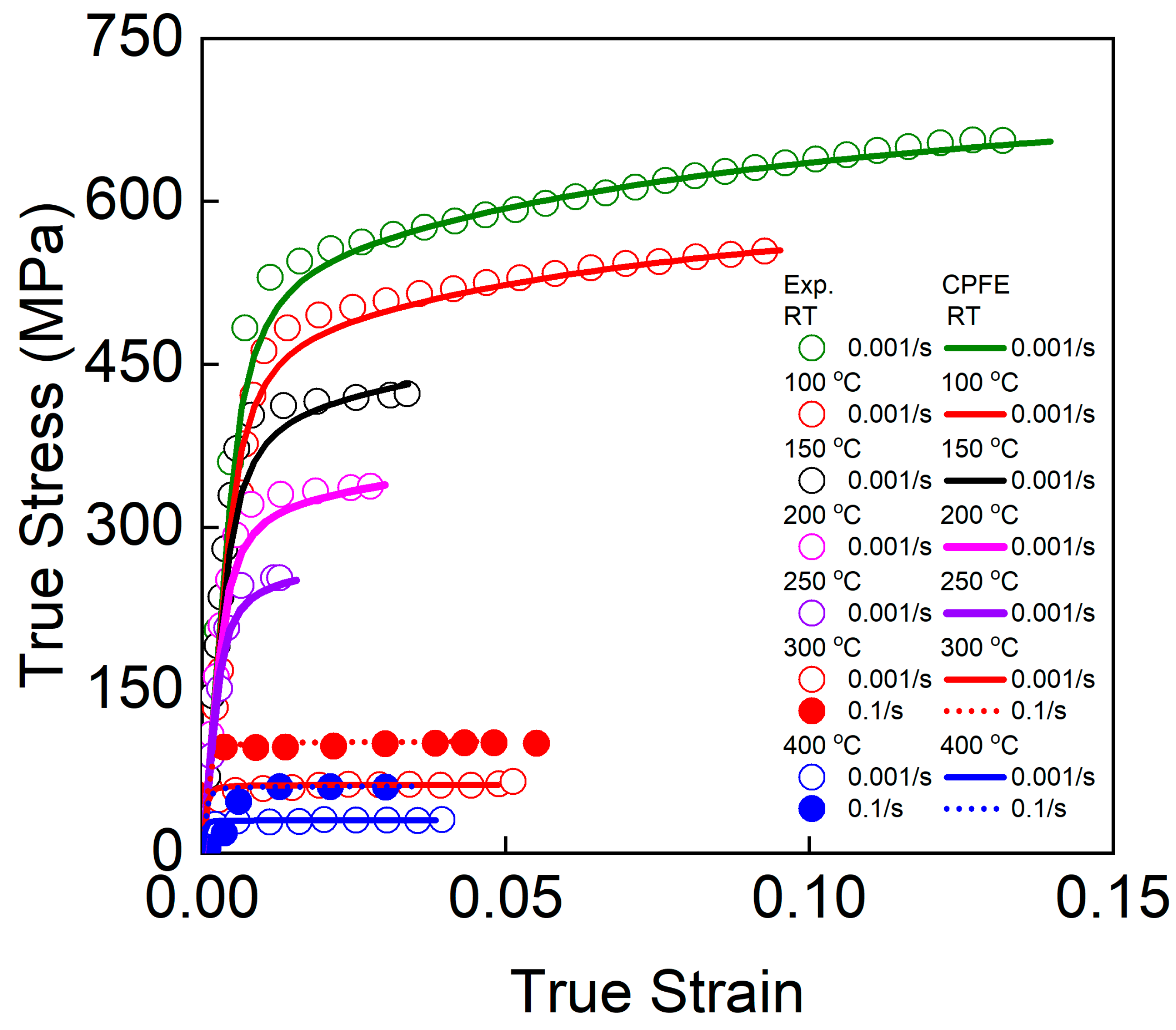
The constitutive parameters of the dislocation density-based crystal plasticity model were calibrated through a trial-and-error procedure to reproduce the experimentally measured stress–strain responses shown in Figure 4. To this end, a three-dimensional cubic representative volume element (RVE) consisting of 1000 finite elements was employed. The RVE was discretized using C3D8R elements, which are 8-node linear brick elements with reduced integration, and the global X, Y, and Z directions correspond to the RD, transverse direction (TD), and normal direction (ND), respectively. This RVE configuration was subsequently used throughout the study for all CPFE simulations.
The crystallographic texture measured by EBSD (Figure 1) was used to reconstruct statistically representative discrete orientations. From the corresponding pole figures, 1000 crystallographic orientations were sampled based on the Bunge Euler angle convention (φ1, Φ, φ2). A single crystallographic orientation was assigned to each integration point, such that each finite element represents an individual grain. Consequently, the RVE represents a polycrystalline aggregate composed of 1000 grains with distinct crystallographic orientations, enabling accurate CPFE simulations of the mechanical response of the AA7075-T6 sheet. The fitting results at different loading conditions are shown in Figure 4, and the corresponding material parameters derived from the fitting are listed in Table 2.
Using the best-fit constitutive parameters listed in Table 2, the scaling factor k ( T ) , which represents the variation of g 0 and k b with temperature, was determined as follows:
g 0 ( T ) k b ( T ) = k ( T ) g 0 ( T 0 ) k b ( T 0 )
k ( T ) = 1 1 + T T 0 h 1 h 2
Here, T 0 denotes room temperature (or 25 °C). h 1 and h 2 were set to 181.5 °C and 3.51, respectively.
According to the literature, the elastic constants of aluminum, i.e., C 11 , C 12 , C 44 , and the shear modulus G are known to vary linearly with temperature in the range from room temperature to approximately 630 °C [29,30]. Based on the data reported in two references, these parameters were expressed by the following linear equations:
C 11 = 107.7 0.0314 T T 0 C 12 = 60.2 + 0.00341 T T 0 C 44 = 28.4 0.0157 T T 0 G = 26.5 0.0157 T T 0
For the strain rate sensitivity, the m value was determined to be 0.14, which provided the best agreement with the experimental results across all temperature and strain rate conditions.

3.2. Hybrid M–K Model

To generate forming limit data based on the crystal plasticity model, a hybrid M–K model is employed. In general, the M–K model assumes two representative regions: the matrix (region A) and the groove region (region B), the latter containing a pre-existing thickness imperfection inclined at an angle ψ . The initial imperfection ratio f 0 (<1) is defined as the ratio between the initial thickness of each region:
f 0 = t B , 0 t A , 0
where t ( i ) , 0 denotes the initial thickness of region (i). The M–K model solves the coupled force equilibrium and strain compatibility conditions between the matrix and groove regions for a given imperfection geometry. From Equation (14), the applied strain path in the matrix induces higher stresses in the imperfection region due to the in-plane force equilibrium across the interface, expressed as follows:
f n n = σ n n A t A = σ n n B t B f n t = σ n t A t A = σ n t B t B
where σ n n ( i ) and σ n t ( i ) represent the normal and shear stresses on the plane normal to the groove orientation of region (i).
The strain compatibility condition along the groove direction must also be satisfied:
d ε t t A = d ε t t B
where ε t t ( i ) denotes the strain component parallel to the groove orientation in region (i). The inclination angle of the groove region is updated incrementally according to the applied strain increment as follows:
tan ψ + d ψ = tan ψ 1 + d ε x x A 1 + d ε y y B
In the present hybrid M–K analysis, the initial inclination angle of the groove region is treated as an independent numerical parameter. For each prescribed strain path, the groove angle is varied from 0° to 90° in increments of 10°, and a full M–K evaluation is performed for each inclination angle. The forming limit strain is then determined as the minimum major strain where localization first occurs among all considered groove angles.
In the hybrid M–K model, the stress–strain response is not evaluated from a macroscopic yield function but from the mechanical response of representative volume elements (RVEs) computed using the CPFE model [21,31,32]. For a prescribed strain path in the matrix, the stress response of region A (RVE-A) is calculated using the CPFE formulation described in Section 3.1. The boundary conditions derived from the equilibrium and compatibility equations (Equations (15) and (16)) are then applied to region B (RVE-B), which represents the imperfection zone.
The forming limit is defined when the strain rate through the thickness of RVE-B becomes at least ten times larger than that of RVE-A, indicating the onset of localized necking. Additional details are given in Section 3.3.

3.3. Numerical Implementation

In this study, CPFE calculations were performed using a fully implicit backward Euler integration algorithm implemented in Abaqus/Standard within a static implicit solution framework. Stress increments associated with plastic deformation were computed using an iterative Newton–Raphson method, requiring a consistently linearized Jacobian matrix compatible with the adopted time integration scheme. The computational procedure for the stress update is summarized in Table 3.
Based on the CPFE results obtained from Abaqus/Standard, the forming limit was evaluated using the hybrid M–K model through a separate post-processing procedure. The corresponding algorithmic steps are summarized in Table 4.

4. Results and Discussion

4.1. FLD: Experiment and Predictions

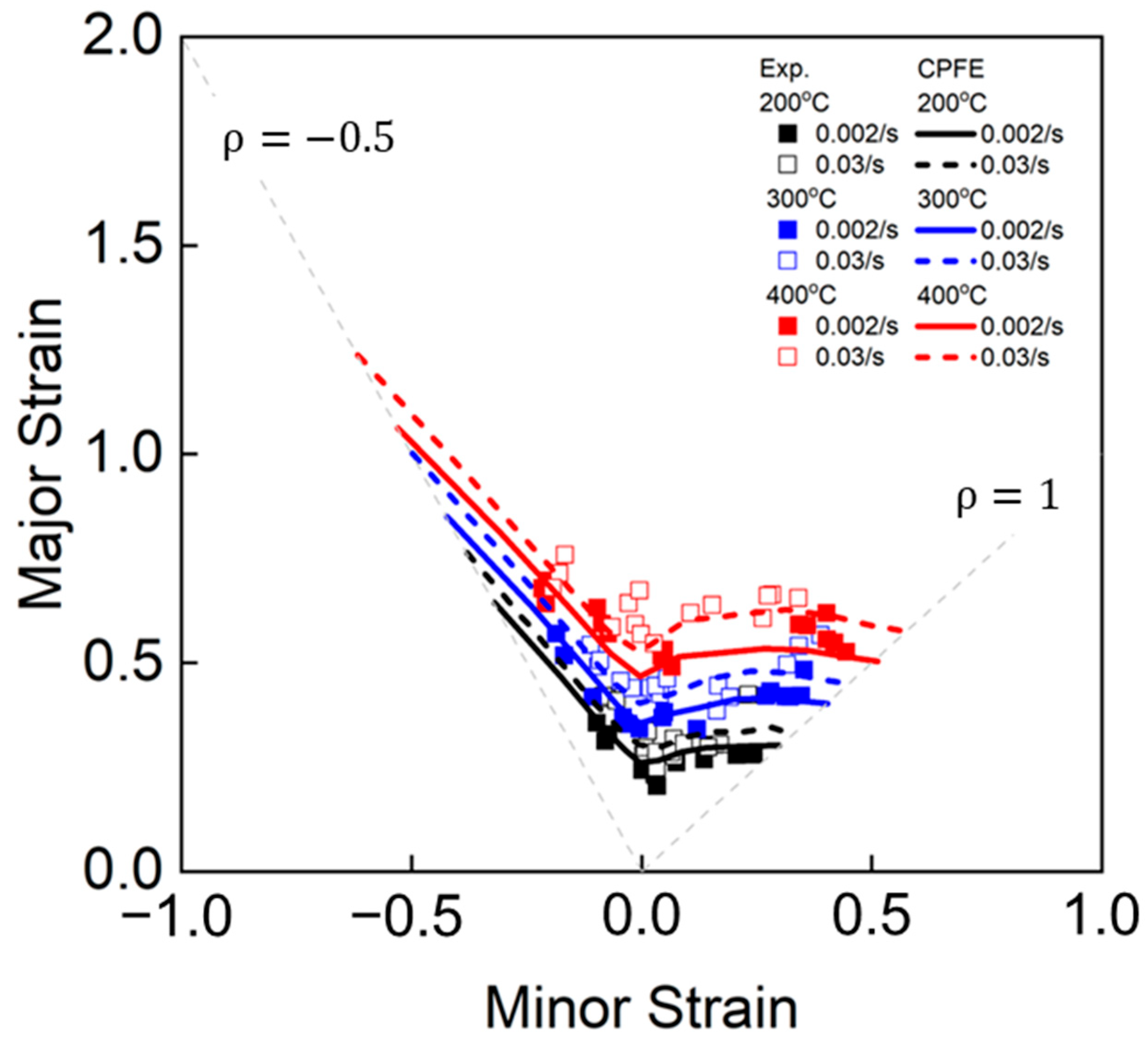
The FLDs obtained from the Nakajima tests described in Section 2.3 are presented in Figure 5 by symbols. The experiments were conducted at three temperatures (200, 300, and 400 °C) and two strain rates (0.002 and 0.03 s−1). For each temperature and strain rate combination, five specimen geometries, shown in Figure 3c representing different strain ratios, were tested three times. Finally, 90 FLD data points were obtained. Experimentally, it is clearly observed that the formability increases with increasing temperature and strain rate. The FLDs were predicted using the hybrid M–K model, which combines the crystal plasticity model and the M–K model described in Section 3. The initial imperfection factor assumed in the M–K model was set to 0.995, and was considered independent of the temperature and strain rate. The FLDs predicted by the hybrid M–K model were compared with the experimental results, as shown in Figure 5. In general, the hybrid M–K model shows good agreement with the experimentally measured FLDs and successfully reproduces the observed enhancement in formability with increasing temperature and strain rate.
As shown in Figure 5, the hybrid M–K model accurately predicted the FLDs of the AA7075-T6 sheet, thereby validating the reliability of the model. To achieve the ultimate objective of this study, predicting FLDs under various temperatures and strain rates using machine learning, additional training data were generated by employing the hybrid M–K model under different temperature and strain rate conditions. Specifically, virtual FLDs were computed at temperatures ranging from 200 to 400 °C in 25 °C increments (total of 9 different temperatures) and at 3 strain rates (0.002, 0.3, and 0.5 s−1), using the 11 strain paths. Finally, 297 virtual FLD data points were generated. Through the aforementioned procedure, a total of 90 experimental datasets corresponding to different strain paths, strain rates, and temperatures, as well as 297 virtual datasets generated from the hybrid M–K model, were obtained and subsequently used for the ML training.

4.2. ML Modeling

4.2.1. Description of ML Models

The aim of the current study was to evaluate the prediction capability of ML algorithm to predict the major strain at necking, ε1, using three independent variables: temperature, strain rate, and strain ratio. ML models can be categorized as follows: linear models, tree-based, probabilistic, kernel-based, and neural network-based. Representative algorithms from each category, i.e., LR, RFR, GPR, SVR, and MLP, were employed for model training. The aim was to evaluate the prediction capability of each algorithm, considering the underlying physical nonlinearity. A brief description of each ML model is provided below.
The LR model assumes a direct linear relationship between the input variables, x, and the target variable, y, which can be expressed as follows:
y = w T x + b + e
where w and b are the model parameters, and e represents the random error term. The model parameters w and b are estimated using the least squares method, which minimizes the following objective function:
min w , b i = 1 n y i w T x i b 2
where n is the number of training samples.
Due to its simplicity, LR provides an excellent baseline for performance comparison and allows for direct interpretation of the influence of each feature. However, since forming parameters such as strain or flow stress are typically nonlinear functions of temperature and strain rate, the LR model struggled to capture complex dependencies. Consequently, while it showed stable and fast convergence, its overall predictive accuracy was limited, particularly in regions exhibiting strain-rate sensitivity or thermally activated deformation mechanisms.
The RFR algorithm is an ensemble method based on multiple decision trees trained on different subsets of the data. Each tree contributes a prediction, and the final forest prediction is obtained by averaging the outputs of all trees, thereby reducing model variance and improving generalization. Mathematically, the random forest predictor y ^ x can be expressed as the average of predictions from T individual regression trees, f i x :
y ^ x = 1 T t = 1 T f i x
Each tree f i x is trained on a bootstrap sample of the training data, and at each split node, a random subset of features is considered to determine the optimal splitting criterion. The split is selected so as to minimize the residual variance of the target values, that is, the mean squared error (MSE) within the child nodes. The impurity at a node t is defined as follows:
I ( t ) = 1 N t j = 1 N t y j y ¯ t 2
where y j denotes the major strain at necking ε1 for sample j and y ¯ t is the mean value in node t. The optimal split maximizes the reduction in this impurity, so that each tree is grown by greedily minimizing the MSE of the residuals between the observed y j values and their node-wise means y ¯ t . This randomness in both data sampling and feature selection effectively decorrelates the trees, thereby reducing model variance compared with a single decision tree.
The hyperparameter T represents the number of trees, and larger values generally reduce variance but increase computational cost. The “maximum depth” parameter controls the maximum allowable depth of each decision tree. When “maximum depth” equals “None”, trees are expanded until all leaves are pure or until they contain fewer samples than required for splitting, corresponding to fully grown trees. The “maximum features” hyperparameter determines the number of input features considered when evaluating candidate splits. The “minimum samples_split” and “minimum samples_leaf” control the minimum number of samples required to perform a split and to form a leaf node, respectively, influencing the smoothness and generalization of each tree.
SVR employs a kernel-based approach that maps the input data into a higher-dimensional feature space, enabling it to capture nonlinear relationships between input features and target outputs. It seeks to find a regression function that approximates the underlying relationship between the input vector x and the target value y while maintaining maximum flatness and tolerating small deviations within an ε-margin. The regression function is defined as follows:
f x = w T ϕ x + c
where ϕ x denotes a nonlinear mapping of the input vector into a higher-dimensional feature space, w is the weight vector, and c is the bias term. SVR minimizes the following regularized risk functional by estimating w and c :
R r e g = 1 2 w 2 + C i = 1 m ξ i + ξ i *
where ξ i and ξ i * are variables that represent the deviations above and below the ε-margin. The residual minimized by SVR is therefore the portion of the prediction error that exceeds the ε -margin, i.e., when
y i f x i > ε .
In this study, the radial basis function (RBF) kernel was used, which is defined as follows:
k x i , x j = exp γ x i x j 2
where the hyperparameter γ controls the width of the kernel and therefore the smoothness of the regression function. In addition, the hyperparameter C (penalty parameter) determines the strength of the regularization term in Equation (23), and ε specifies the width of the insensitive zone within which prediction errors are not penalized.
GPR is a probabilistic non-parametric learning method that models the target response as a distribution over functions. For an input vector x * , the predictive distribution of GPR is defined by the posterior mean and covariance functions:
y ^ = m p x *
V a r y ^ = k p x * , x *
where m p and k p denote the posterior predictive mean and covariance functions, respectively.
The covariance between samples is governed by a kernel function k x i , x j , which determines the smoothness and correlation structure of the response surface. In this study, the RBF kernel was used:
k x i , x j = σ f 2 exp x i x j 2 2 l 2
where l is the characteristic length scale and σ f 2 is the signal variance. A WhiteKernel component is added to model observation noise with variance σ n 2 , leading to the combined kernel:
k t o t a l x i , x j = k R B F x i , x j + σ n 2 δ i j
To optimize the kernel hyperparameters, GPR maximizes the log marginal likelihood:
log p y X , θ = 1 2 y T K 1 y + 1 2 log K + n 2 log 2 π
where K is the kernel matrix and θ denotes the kernel hyperparameters. In Equation (30), the first term captures the residual fitting error, the second penalizes model complexity, and the third is a normalization constant. Regularization noise ( α ) corresponds to a small value added to the diagonal of K to improve numerical stability. Length scale (l) controls the smoothness of the RBF kernel, determining how rapidly correlations decay with distance. Noise variance ( σ n 2 ) governs the magnitude of the WhiteKernel contribution and represents observation noise.
The MLP, a type of artificial neural network, is a fully connected feed-forward neural network that approximates nonlinear mappings between the input variables and the target response. The MLP consists of an input layer, several hidden layers, and an output layer. For an input vector x, the forward propagation through layer l is written as follows:
h l = σ W l h l 1 + b l , l = 1 , 2 , ... , L
where W l and b l denote the weight matrix and bias vector of layer l, h l 1 is the output of the previous layer, and σ is the activation function. In this study, the rectified linear unit (ReLU) function was used as the activation function. The output layer produces the final prediction y ^ of the major strain at necking.
The training of the MLP is carried out by minimizing the MSE between the predicted and observed values:
min Θ 1 N i = 1 N y i y ^ i 2
where N is the number of training samples. During training, gradients of the loss function with respect to the network parameters are computed via backpropagation, and the parameters are updated iteratively using the Adam optimization algorithm.
The hyperparameters tuned during grid search included the number of hidden layers, the number of hidden units per layer, the learning rate, the batch size, the dropout ratio, and the number of training epochs. The number of hidden layers and units determines the model capacity and its ability to represent nonlinear relationships, while the learning rate and batch size control the optimization behavior during training. The dropout ratio is used to prevent overfitting by randomly deactivating a portion of neurons, and the number of epochs specifies how many times the training dataset is iterated during optimization.

4.2.2. Predictions Using ML Models

In this study, the strain rate, temperature, and strain ratio were set as the input variables for the ML models, while the major strain at necking, ε1, was defined as the output variable. Two types of FLD datasets were used to train the ML models and predict the FLD: (a) 90 experimental datasets obtained from experiments, and (b) a combined dataset consisting of 90 experimental data points and 297 additional data points generated using the hybrid M–K model. The entire dataset was divided into training, validation, and test sets with a ratio of 6:2:2 to ensure reliable model training and evaluation. The training dataset was used to optimize the model parameters by minimizing the loss function during the learning process. The validation dataset served to tune the model’s hyperparameters and assess its performance during development, preventing overfitting by providing feedback on unseen data not directly involved in parameter updates. Finally, the test dataset, which was completely excluded from both training and validation stages, was employed to evaluate the model’s predictive capability and generalization performance on entirely new data.
The root mean square error (RMSE) was used as the objective function for the ML models. The RMSE was calculated using the following equation.
R M S E = 1 n i = 1 n y i t i 2
where n is the total number of data values; yi and ti are the predicted and data values used for ML training.
To improve the accuracy of the ML models, hyperparameter tuning was performed. For this purpose, the well-known grid search cross-validation (CV) method was employed. It exhaustively searches through a predefined grid of parameter combinations and evaluates each configuration using CV to estimate model performance. The parameter set that yields the best validation score is then selected as the optimal hyperparameter configuration, ensuring a more robust and generalized model performance. The optimal hyperparameters of the ML models determined using the grid search CV algorithm, along with the corresponding hyperparameter search ranges explored during the tuning process, are summarized in Table 5. It is worthwhile to note that the LR model does not have any hyperparameters to be optimized; therefore, no hyperparameter tuning was performed for this model.
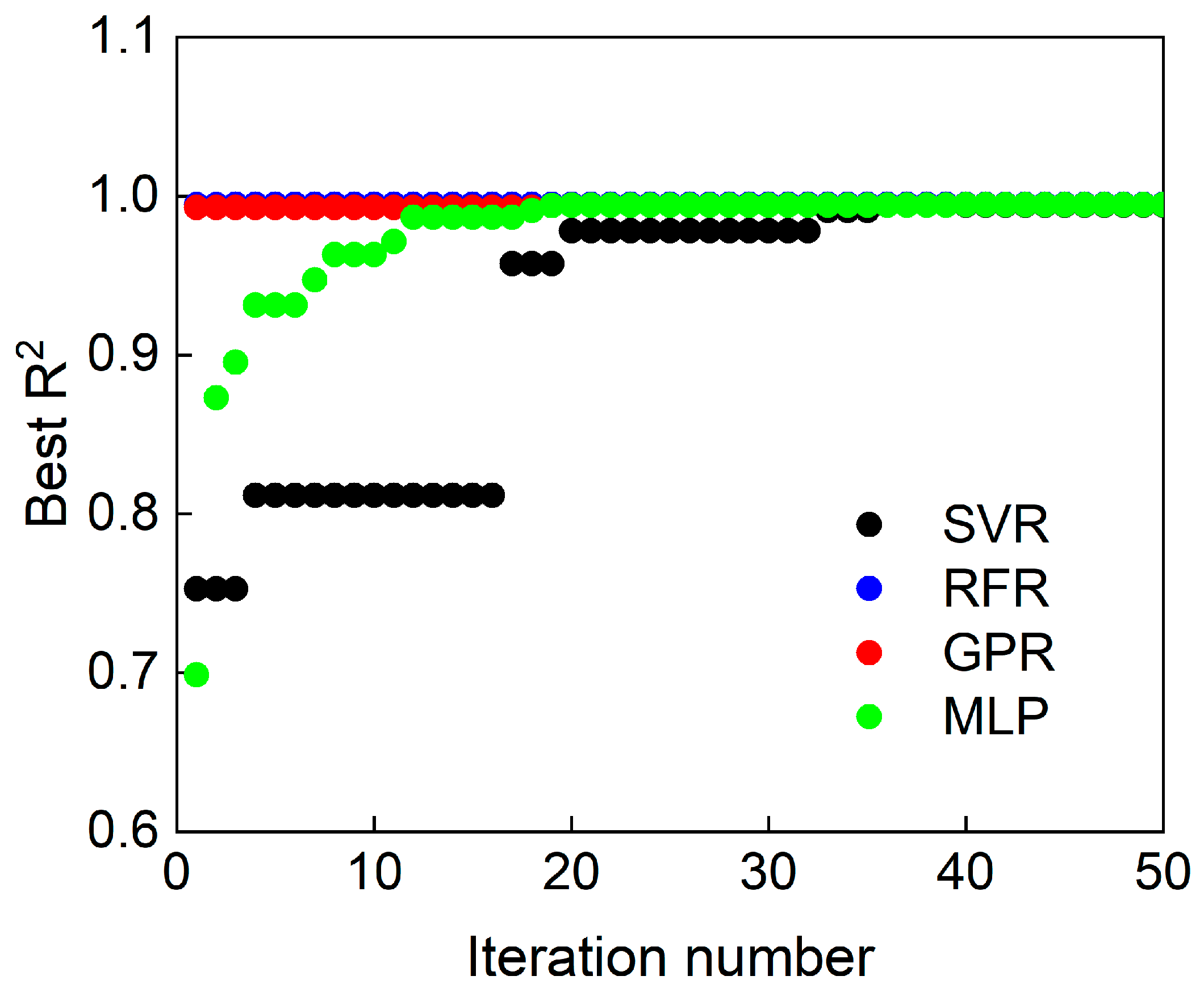
Figure 6 illustrates the evolution of the best-so-far cross-validated R2 during the hyperparameter optimization process for nonlinear machine learning models. The R2 value at each iteration represents the highest validation performance achieved among all hyperparameter combinations evaluated up to that point. The results reveal distinct convergence behaviors among the models. RFR and GPR achieve near-optimal R2 values from the early stages of the optimization, indicating that their default configurations already provide strong nonlinear representational capacity for the present dataset. In contrast, SVR and MLP exhibit a gradual increase in R2 as the hyperparameter search progresses, reflecting their higher sensitivity to hyperparameter selection and the need for iterative tuning to reach optimal performance.
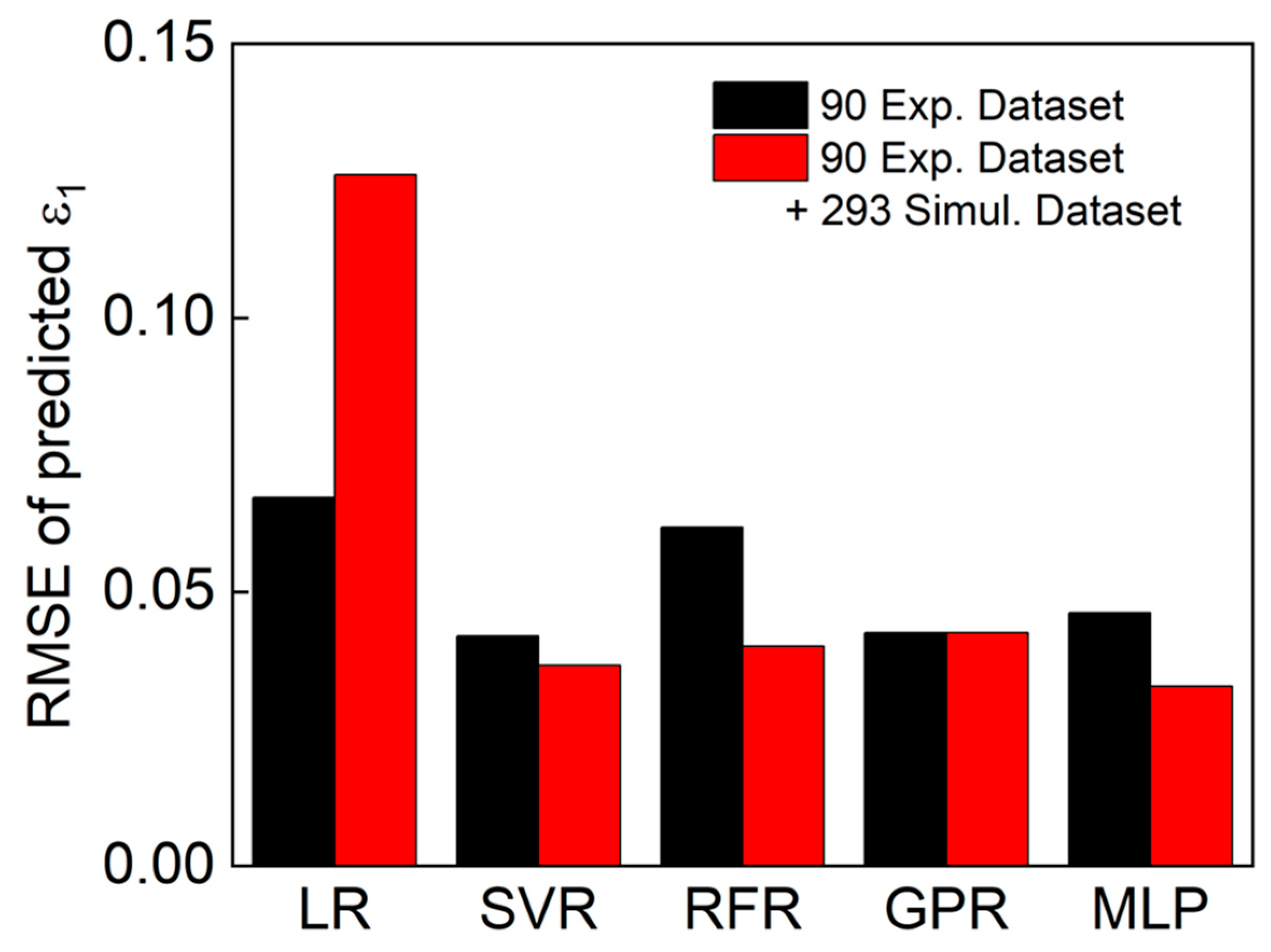
Figure 7 compares the results using the RMSE, calculated using the validation dataset, between the training data used for the ML models and the predictions obtained from the trained ML models. In the LR model, the error appeared to be the largest, which is likely due to the nonlinear relationship between the input and output data. An interesting observation from the LR results is that when the dataset size is relatively small, the RMSE value tends to be lower; this will be further discussed in the following section comparing the R2 results. Except for the LR model, most other ML models exhibited a general trend in which the RMSE value decreased as the number of training data points increased. Regardless of the specific ML model used, all models showed significantly lower RMSE values compared to the LR model.
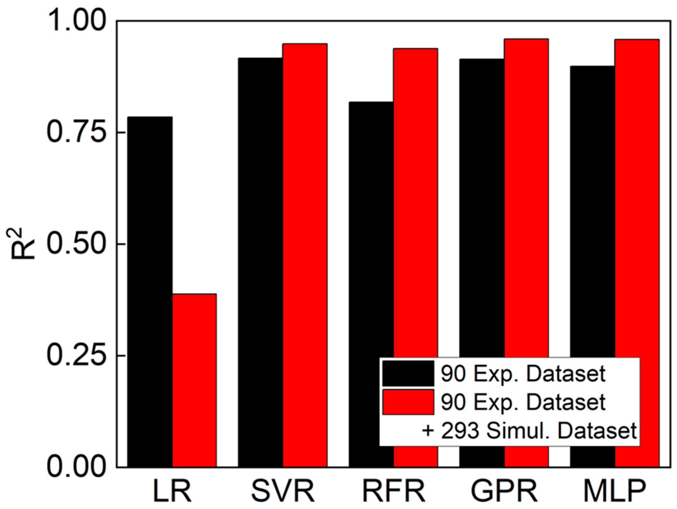
In addition to the comparison using RMSE values, the predicted major strain at necking (ε1) obtained from the ML models was compared using R2 analysis with the validation dataset. Figure 8 presents a comparison between the training data used for the ML models and the corresponding predictions. It is worthwhile to note that RMSE is used to compare absolute prediction errors among the ML models, whereas R2, shown in Figure 8, provides a scale-independent measure of predictive performance that is not affected by the magnitude of ε 1 . As shown in the results, the LR model exhibited lower prediction accuracy compared to the other ML models, and its prediction accuracy tended to improve as the number of datasets increased. For the other ML models excluding LR, the overall R2 values were higher than 0.89, and when a larger number of training data points (90 experimental datasets + 293 simulation datasets) were used, the prediction accuracy further improved, yielding R2 values exceeding 0.93. Among all models, the GPR model showed the highest prediction accuracy in the R2 analysis, with R2 values ranging from 0.9139 to 0.9596.
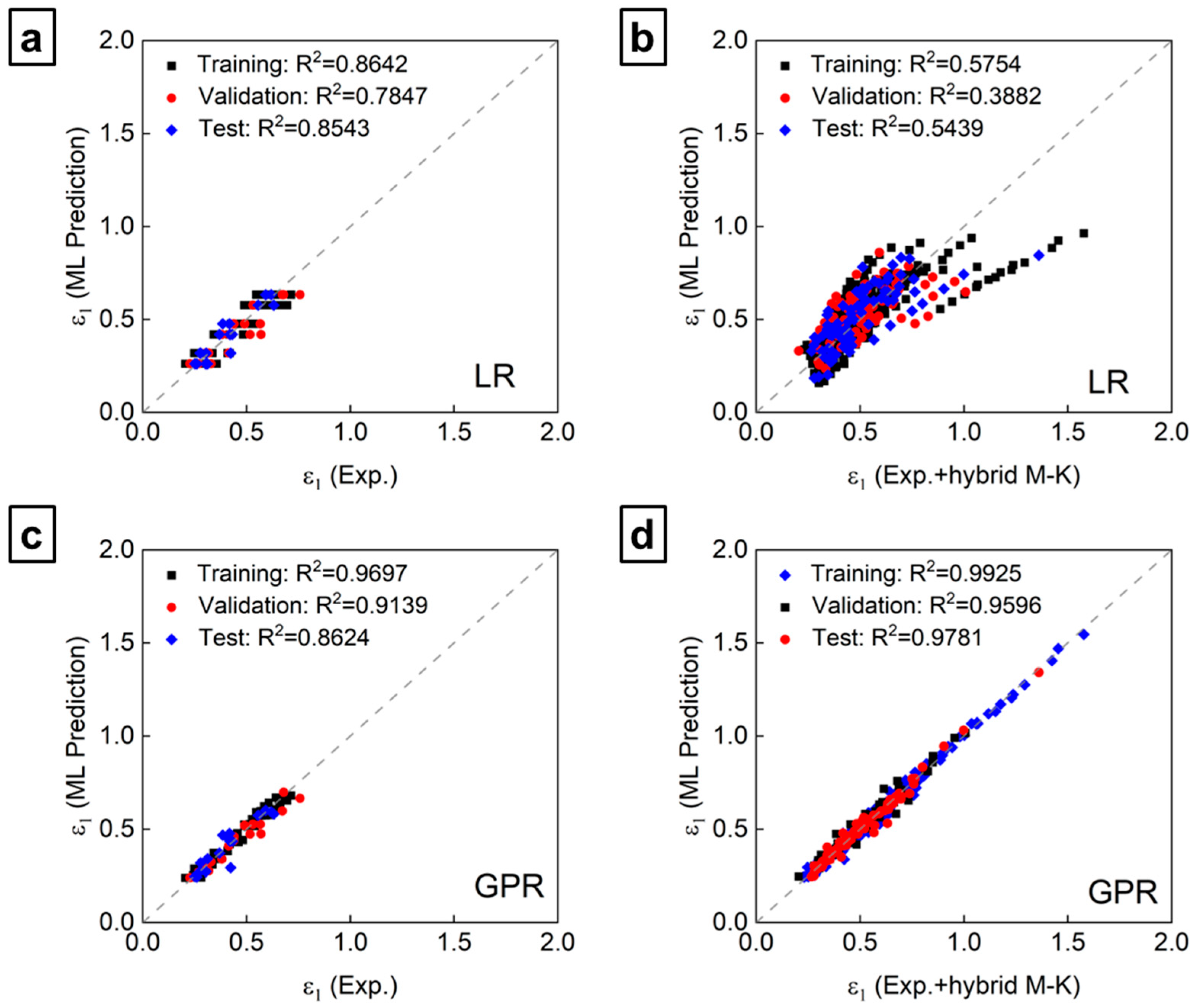
From the results of the previous RMSE and R2 analyses, it was observed that the LR model exhibited a noticeable decrease in prediction accuracy when a larger number of training data points were used. To further analyze this behavior, the predicted results of the ML models were compared one-to-one with the training data, as shown in Figure 9. For comparison, the results of the GPR model, which showed the highest prediction accuracy in the R2 analysis, were also plotted. The GPR model, which demonstrated high prediction accuracy, showed that the test datasets lie approximately along the linear y = x line and are closely aligned with the validation and training data, regardless of the number of training samples. The best R2 value for the test dataset was 0.9781, which means great predictability of the ML model. In contrast, for the LR model, when only the 90 experimental datasets were used for training, the predicted and actual data exhibited a roughly one-to-one correspondence. However, when both the 90 experimental data points and 293 data points predicted using the hybrid M–K model were used for training, the predicted results deviated significantly from the training data. This discrepancy can be attributed to the limited range of strain rates in the experimental data (0.002–0.03/s) due to experimental equipment constraints, compared to the wider range of the hybrid M–K model predictions (0.002–0.5/s). As the strain rate increases, the formability (i.e., the value of ε1) tends to increase, and the relationship between the input variables (temperature, strain rate, and strain ratio) and the output variable (ε1) becomes more nonlinear, which likely causes the reduced prediction accuracy of the LR model.
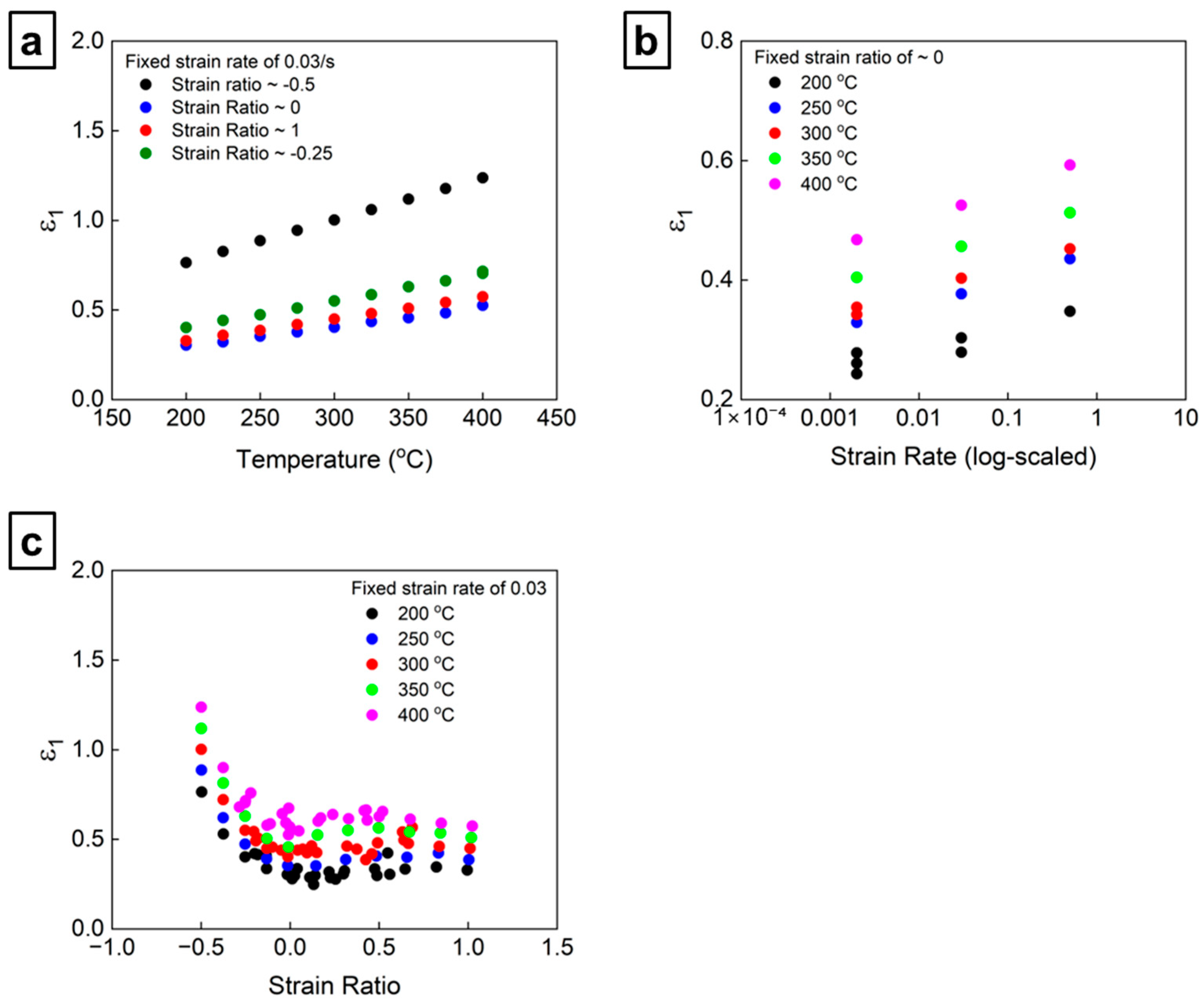
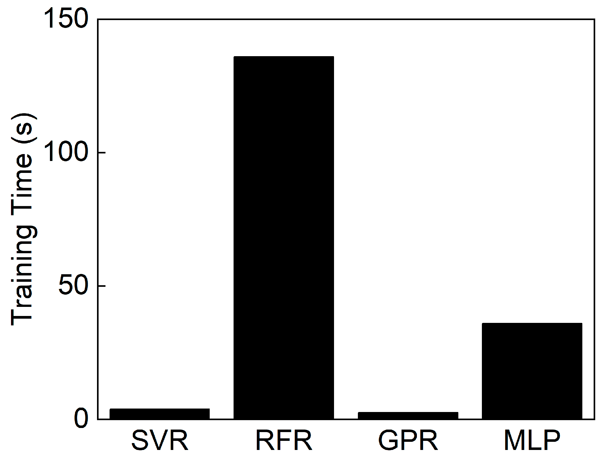
The reported training times correspond to the final model fitting using the optimal hyperparameters obtained from the grid search procedure. As shown in the figure, SVR and GPR exhibit the shortest training times, both completing the training process within only a few seconds. In contrast, MLP requires a noticeably longer training time, while RFR shows a substantially higher computational cost, resulting in the longest training time among all models. These results indicate a clear hierarchy in computational efficiency across the examined nonlinear regression approaches. To more clearly illustrate the inherent nonlinear behavior of the forming limit dataset, the dependence of the major strain at necking (ε1) on the individual input parameters was examined while keeping the remaining variables constant. For this purpose, a subset of representative data points was selected from the full set of 383 experimental and simulation-derived samples, and the relationships between each input parameter and ε1 were visualized. Figure 10a shows the variation of ε1 with temperature at a fixed strain rate, and Figure 10b presents ε1 as a function of strain rate under fixed temperature and strain-ratio conditions. From these two figures, it is evident that the input parameters (temperature and strain rate) and the target value (ε1) exhibit a highly nonlinear relationship. However, as shown in Figure 10c, the other input parameter, the strain ratio, exhibits a strongly nonlinear relationship with the target value ε1. These observations justify the necessity of nonlinear ML models for accurate FLD prediction and explain the performance differences observed in Figure 7 and Figure 9.
Figure 11 presents a comparison of the training time required for the four nonlinear machine learning models considered in this study, namely SVR, RFR, GPR, and MLP. As shown in the figure, SVR and GPR exhibit the shortest training times, both completing the training process within only a few seconds. In contrast, MLP requires a noticeably longer training time, while RFR shows a substantially higher computational cost, resulting in the longest training time among all models. These results indicate a clear hierarchy in computational efficiency across the examined nonlinear regression approaches.
The differences in training time among the models arise from their inherent computational characteristics. SVR and GPR are kernel-based methods, for which the final training involves a single optimization step after fixing the hyperparameters. For the dataset size considered, kernel matrix operations can be efficiently handled, resulting in short training times. In contrast, MLP relies on iterative gradient-based optimization via backpropagation, and its training time increases with the number of epochs and trainable parameters, leading to moderately higher computational costs. RFR shows the longest training time due to the cumulative cost of building multiple decision trees, each involving repeated node splitting and feature selection. Consequently, the observed training time hierarchy (SVR ≈ GPR < MLP < RFR) is consistent with the computational complexity and training mechanisms of the respective models.

5. Conclusions

In this study, a hybrid data-driven approach was developed to predict the forming limit diagrams (FLDs) of AA7075-T6 aluminum sheets under various temperatures and strain rates. Since experimental determination of FLDs is often limited by the high cost and time required for testing, virtual data were additionally generated through rate-dependent crystal plasticity finite element (CPFE) simulations coupled with the Marciniak–Kuczyński (M–K) model. These simulation results were combined with experimentally measured FLDs to construct a comprehensive dataset for machine learning (ML) training. Several ML models, including linear regression (LR), support vector regression (SVR), random forest regression (RFR), Gaussian process regression (GPR), and multilayer perceptron (MLP), were trained and evaluated to identify the most accurate predictive model. The GPR model exhibited the best performance, effectively capturing the nonlinear dependencies of the forming limit on temperature and strain rate. The key findings of this study are as follows:
  • The hybrid M–K model incorporating the CPFE framework accurately reproduced the experimentally observed trends in FLD, including the enhanced formability with increasing temperature and strain rate.
  • Virtual FLD data generated from the hybrid M–K simulations were combined with the experimental results to construct a comprehensive dataset, enabling robust ML model training.
  • Among the evaluated ML algorithms, the Gaussian process regression (GPR) model demonstrated the best predictive performance (R2 > 0.95), effectively learning the nonlinear relationships between temperature, strain rate, and strain ratio.
  • The integrated hybrid M–K–ML methodology provides a physically informed and computationally efficient framework for predicting the formability of AA7075-T6 across wide thermo-mechanical conditions and can be extended to other anisotropic and rate-sensitive alloys.

Author Contributions

Conceptualization, H.J.B., S.C. and K.M.M.; methodology, H.J.B. and K.M.M.; software, H.J.B.; validation, H.J.B.; formal analysis, H.J.B.; investigation, H.J.B.; resources, H.J.B.; data curation, S.C. and K.M.M.; writing—original draft preparation, H.J.B.; writing—review and editing, S.C. and K.M.M.; visualization, K.M.M.; supervision, H.J.B.; project administration, H.J.B.; funding acquisition, H.J.B. All authors have read and agreed to the published version of the manuscript.

Funding

This work was supported by the New Faculty Research Support Grant from Gyeongsang National University in 2025, GNU-NFRSG-0009 and the Fundamental Research Program of the Korea Institute of Materials Science (KIMS, PNKA300).

Data Availability Statement

The raw data supporting the conclusions of this article will be made available by the authors on request.

Acknowledgments

The authors are grateful for the technical support of Kyung Jae Kim.

Conflicts of Interest

The authors declare no conflicts of interest.

Abbreviations

The following abbreviations are used in this manuscript:
FLDforming limit diagram
M–KMarciniak–Kuczyński
CPFEcrystal plasticity finite element
MLmachine learning
LRlinear regression
RFRrandom forest regression
SVRsupport vector regression
GPRGaussian process regression
MLPmultilayer perceptron
RDrolling direction
MSEmean square error
RMSEroot mean square error
CVcross-validation

References

  1. Xu, T.; Li, F.; Wang, X.; Zhang, G. Characterization of Anisotropic Fracture Behavior of 7075-T6 Aluminum Alloy Sheet under Various Stress States. J. Mater. Eng. Perform. 2022, 32, 3230–3252. [Google Scholar] [CrossRef]
  2. Sajadifar, S.V.; Scharifi, E.; Weidig, U.; Steinhoff, K.; Niendorf, T. Performance of Thermo-Mechanically Processed AA7075 Alloy at Elevated Temperatures—From Microstructure to Mechanical Properties. Metals 2020, 10, 884. [Google Scholar] [CrossRef]
  3. Moon, C.; Thuillier, S.; Lee, J.; Lee, M.G. Mechanical Properties of Solution Heat Treated Al-Zn-Mg-Cu (7075) Alloy under Different Cooling Conditions: Analysis with Full Field Measurement and Finite Element Modeling. J. Alloys Compd. 2021, 856, 158180. [Google Scholar] [CrossRef]
  4. Wang, H.; Luo, Y.B.; Friedman, P.; Chen, M.H.; Gao, L. Warm Forming Behavior of High Strength Aluminum Alloy AA7075. Trans. Nonferrous Met. Soc. China 2012, 22, 1–7. [Google Scholar] [CrossRef]
  5. Zhou, M.; Lin, Y.C.; Deng, J.; Jiang, Y.Q. Hot Tensile Deformation Behaviors and Constitutive Model of an Al–Zn–Mg–Cu Alloy. Mater. Des. 2014, 59, 141–150. [Google Scholar] [CrossRef]
  6. Sotirov, N.; Simon, P.; Chimani, C.; Uffelmann, D.; Melzer, C. Warm Deep Drawability of Peak-Aged 7075 Aluminium Sheet Alloy. Key Eng. Mater. 2012, 504–506, 955–960. [Google Scholar] [CrossRef]
  7. Khan, A.S.; Baig, M. Anisotropic Responses, Constitutive Modeling and the Effects of Strain-Rate and Temperature on the Formability of an Aluminum Alloy. Int. J. Plast. 2011, 27, 522–538. [Google Scholar] [CrossRef]
  8. Li, D.; Ghosh, A. Tensile Deformation Behavior of Aluminum Alloys at Warm Forming Temperatures. Mater. Sci. Eng. A 2003, 352, 279–286. [Google Scholar] [CrossRef]
  9. Rader, K.E.; Carter, J.T.; Hector, L.G.; Taleff, E.M. Plastic Deformation and Ductility of AA7075 and AA6013 at Warm Temperatures Suitable to Retrogression Forming. Metall. Mater. Trans. A 2021, 52, 4003–4017. [Google Scholar] [CrossRef]
  10. Rong, H.; Hu, P.; Ying, L.; Hou, W.; Zhang, J. Thermal Forming Limit Diagram (TFLD) of AA7075 Aluminum Alloy Based on a Modified Continuum Damage Model: Experimental and Theoretical Investigations. Int. J. Mech. Sci. 2019, 156, 59–73. [Google Scholar] [CrossRef]
  11. Min, K.M.; Kim, C.; Choi, S.; Hong, J.H.; Lee, J.; Bong, H.J. Forming Limit Diagram of an Ultra-Thin Commercially Pure Titanium Sheet: Combined Experimental–Numerical Approach. J. Mater. Res. Technol. 2025, 39, 7110–7123. [Google Scholar] [CrossRef]
  12. Yatkın, M.A.; Kõrgesaar, M. Machine Learning Enabled Identification of Sheet Metal Localization. Int. J. Solids Struct. 2024, 288, 112592. [Google Scholar] [CrossRef]
  13. Li, X.; Roth, C.C.; Mohr, D. Neural Network Based Rate- and Temperature-Dependent Hosford–Coulomb Fracture Initiation Model. Int. J. Mech. Sci. 2023, 260, 108643. [Google Scholar] [CrossRef]
  14. Samad, A.; Thakur, A.K.; Basak, S.; Pal, K. Machine Learning Enabled Estimation of Formability for Anisotropic Sheet Metals. Met. Mater. Int. 2025, 1–25. [Google Scholar] [CrossRef]
  15. Nguyen, N.T.; Tran, M.T.; Nguyen, X.M.; Lee, H.W.; Kang, S.H.; Oh, Y.S.; Kim, H.; Kim, D.K. Physics-Guided Machine Learning for Forming-Limit Assessments of Advanced High-Strength Steels. Int. J. Mech. Sci. 2025, 287, 109959. [Google Scholar] [CrossRef]
  16. Jaremenko, C.; Ravikumar, N.; Affronti, E.; Merklein, M.; Maier, A. Determination of Forming Limits in Sheet Metal Forming Using Deep Learning. Materials 2019, 12, 1051. [Google Scholar] [CrossRef]
  17. Chheda, A.M.; Nazro, L.; Sen, F.G.; Hegadekatte, V. Prediction of Forming Limit Diagrams Using Machine Learning. In Proceedings of the IOP Conference Series: Materials Science and Engineering; IOP Publishing: Bristol, UK, 2019; Volume 651, p. 12107. [Google Scholar]
  18. Lv, L.; Lee, W.W.; Lin, H.; Jin, T. Plastic Anisotropy of AA7075-T6 Alloy under Quasi-Static Compression: Experiments, Classical Plasticity and Artificial Neural Networks Modeling. Appl. Phys. A Mater. Sci. Process. 2023, 129, 209. [Google Scholar] [CrossRef]
  19. Steglich, D.; Jeong, Y. Texture-Based Forming Limit Prediction for Mg Sheet Alloys ZE10 and AZ31. Int. J. Mech. Sci. 2016, 117, 102–114. [Google Scholar] [CrossRef]
  20. Tran, M.T.; Lee, H.J.; Phan, H.C.; Kang, S.H.; Kim, D.K.; Lee, H.W. Microstructure-Informed Forming Limits in Aluminum Alloys: Experiments and Crystal Plasticity Simulations. Mater. Charact. 2025, 230, 115831. [Google Scholar] [CrossRef]
  21. Kim, J.H.; Lee, M.G.; Kang, J.H.; Oh, C.S.; Barlat, F. Crystal Plasticity Finite Element Analysis of Ferritic Stainless Steel for Sheet Formability Prediction. Int. J. Plast. 2017, 93, 26–45. [Google Scholar] [CrossRef]
  22. Hajian, M.; Assempour, A. Experimental and Numerical Determination of Forming Limit Diagram for 1010 Steel Sheet: A Crystal Plasticity Approach. Int. J. Adv. Manuf. Technol. 2015, 76, 1757–1767. [Google Scholar] [CrossRef]
  23. Rohoman, M.M.; Zhou, C. Crystal Plasticity Modeling of Dislocation Density Evolution in Cellular Dislocation Structures. Metals 2025, 15, 419. [Google Scholar] [CrossRef]
  24. Wu, L.; Duan, W.; Zhang, S.; Yang, X.; Li, W.; Shen, X.; Zhang, Y.; Zhou, J. Finite Element Simulation of Crystal Plasticity in the Tensile Fracture Behavior of PBF-LB/M CoCrFeNiMn High Entropy Alloy. Metals 2025, 15, 990. [Google Scholar] [CrossRef]
  25. Wang, H.; Dong, J.; Yao, S.; Liu, S.; Cao, L.; Huang, X. Effect of External Constraints on Deformation Behavior of Aluminum Single Crystals Cold-Rolled to High Reduction: Crystal Plasticity FEM Study and Experimental Verification. Metals 2025, 15, 885. [Google Scholar] [CrossRef]
  26. Zeng, G.; Huang, Z.; Deng, B.; Ge, R. Crystal Plasticity Finite Element Simulation of Tensile Fracture of 316L Stainless Steel Produced by Selective Laser Melting. Metals 2025, 15, 567. [Google Scholar] [CrossRef]
  27. Mitreiro, D.; Prates, P.A.; Andrade-Campos, A. Reducing Mesh Dependency in Dataset Generation for Machine Learning Prediction of Constitutive Parameters in Sheet Metal Forming. Metals 2025, 15, 534. [Google Scholar] [CrossRef]
  28. ISO 12004-2; Metallic Materials—Sheet and Strip—Determination of Forming-Limit Curves—Part 2: Determination of Forming-Limit Curves in the Laboratory. International Organization for Standardization: Geneva, Switzerland, 2008.
  29. Davoudi, K. Temperature Dependence of the Yield Strength of Aluminum Thin Films: Multiscale Modeling Approach. Scr. Mater. 2017, 131, 63–66. [Google Scholar] [CrossRef]
  30. Tallon, J.L.; Wolfenden, A. Temperature Dependence of the Elastic Constants of Aluminum. J. Phys. Chem. Solids 1979, 40, 831–837. [Google Scholar] [CrossRef]
  31. Gupta, A.; Ben Bettaieb, M.; Abed-Meraim, F.; Kalidindi, S.R. Computationally Efficient Predictions of Crystal Plasticity Based Forming Limit Diagrams Using a Spectral Database. Int. J. Plast. 2018, 103, 168–187. [Google Scholar] [CrossRef]
  32. Mekonen, M.N.; Steglich, D.; Bohlen, J.; Stutz, L.; Letzig, D.; Mosler, J. Experimental and Numerical Investigation of Mg Alloy Sheet Formability. Mater. Sci. Eng. A 2013, 586, 204–214. [Google Scholar] [CrossRef]
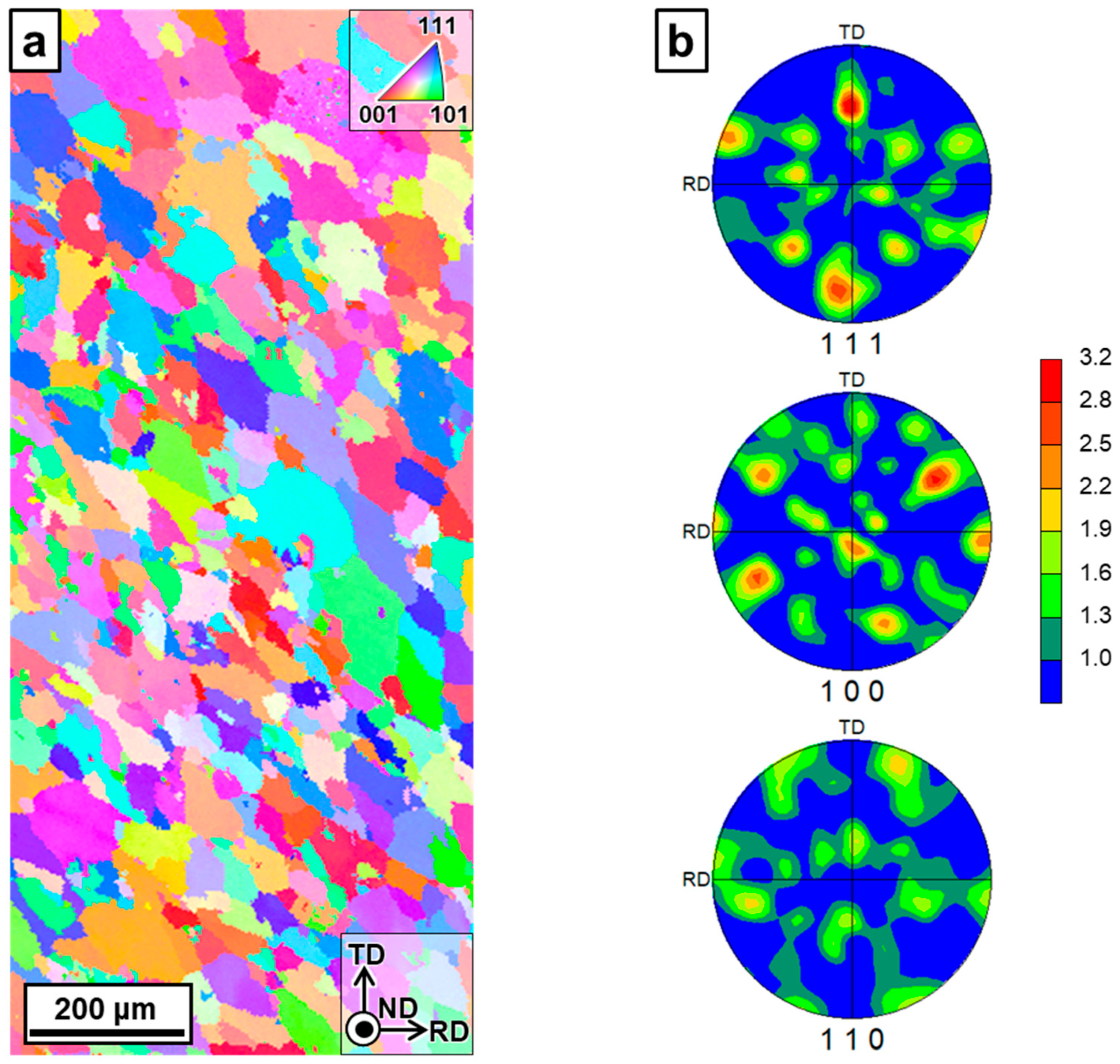
Figure 1. EBSD-characterized microstructure of the as-received AA7075-T6 sheet, showing (a) the ND-IPF map on the RD–TD plane and (b) the corresponding {111}, {100}, and {110} pole figures.
Metals 16 00021 g001
Figure 2. (a) Universal testing machine equipped with a furnace, and (b) geometry and dimensions (in mm) of the specimen used for uniaxial tensile tests.
Metals 16 00021 g002
Figure 3. (a) Experimental setup, (b) Erichsen universal sheet metal testing machine (Erichsen 142-60) equipped with induction heating system, and (c) specimen geometry (in mm) used for Nakajima test.
Metals 16 00021 g003
Figure 4. Experimental and CPFE-fitted true stress–strain curves at various temperatures and strain rates.
Metals 16 00021 g004
Figure 5. Comparison of FLDs of AA7075-T6 alloy at various temperatures and strain rates: experimental data and predictions using hybrid M–K model.
Metals 16 00021 g005
Figure 6. Evolution of the best-so-far cross-validated R2 during hyperparameter optimization for different ML models.
Metals 16 00021 g006
Figure 7. RMSE of predicted major strain at necking, ε1, by various ML models.
Metals 16 00021 g007
Figure 8. R2 of predicted major strain at necking, ε1, by various ML models.
Metals 16 00021 g008
Figure 9. Comparison between ML model predicted and actual major strain at necking: (a) LR predicted vs. experimental data, (b) LR predicted vs. experimental + hybrid M–K predicted data, (c) GPR predicted vs. experimental data, and (d) GPR predicted vs. experimental + hybrid M–K predicted data.
Metals 16 00021 g009
Figure 10. Systematic visualization of the nonlinear dependence of the major strain at necking (ε1) on the input parameters: (a) ε1 versus temperature at a fixed strain rate of 0.03 s−1 for several strain ratios, (b) ε1 versus strain rate (log scale) at an approximately constant strain ratio of 0 for different temperatures, and (c) ε1 versus strain ratio at a fixed strain rate of 0.03 s−1 for different temperatures.
Metals 16 00021 g010
Figure 11. Comparison of the training time required for SVR, RFR, GPR, and MLP models.
Metals 16 00021 g011
Table 1. Chemical compositions of AA7075-T6 (wt%).
Elementwt%
Zn5.1–6.1
Mg2.1–2.9
Cu1.2–2.0
Cr0.18–0.28
Si<0.40
Fe<0.50
Mn<0.30
Ti<0.20
AlBal.
Table 2. Best-fit constitutive parameters at different temperatures for the AA7075-T6 alloy using the CPFE model ( b : magnitude of Burgers vector = 0.286 nm).
Temperature (°C) g 0 (MPa) ρ 0 (m−2) k a k b
251752 × 10131232 b
10015436.4 b
15013043.2 b
20099.856.1 b
25075.374 b
30012.3457 b
4001.753200 b
4700.17532,000 b
Table 3. Algorithmic framework for stress update in CPFE model.
Let τ = t + Δ t .
Given:
   (1) F ( t ) , F ( τ ) for each element
   (2) F p ( t ) , ρ α ( t ) in each grain
   (3) ( s 0 α , n 0 α ) —time independent quantities, for each grain
1. Calculate trial stress
    S e , t r i a l τ = C e E e , t r i a l τ = C e : 1 2 F e T , t r i a l ( τ ) F e , t r i a l ( τ ) I
    where F e , t r i a l ( τ ) = F ( τ ) F p 1 ( t )
2. Update stress in each grain
   Solve G n τ = S n e τ C e : 1 2 F n e T ( τ ) F n e ( τ ) I = 0
   Newton–Raphson method S n + 1 e S n e + G n S n e 1 G n
   where F n e ( τ ) = F ( τ ) F n p 1 ( τ ) = F ( τ ) F p 1 ( t ) I Δ t L n p τ
   2.1. Update dislocation density
    Δ ρ α = 1 b β = 1 N ρ β k a k b ρ α Δ γ α where Δ γ α = γ ˙ 0 s τ α g α ( 1 / m ) sgn τ α
   2.2. Update plastic deformation gradient
    Δ t L n P τ = α Δ γ α s 0 α n 0 α
3. Convergence check
   If  S n + 1 e τ S n e τ < T O L  then:
   Cauchy stress σ τ = 1 det F e ( τ ) F e ( τ ) S e ( τ ) F e T ( τ )
4. Update crystal orientation
    s τ α = F e τ s 0 α , n τ α = F e T τ n 0 α
Table 4. Schematic algorithm for hybrid M–K implementation with CPFE model.
1. Initialization
    1.1 .   Input :   f 0 , ψ , ρ
   1.2. Set initial stress, strain in RVE-A and RVE-B to zero.
    1.3 .   Set   the   macroscopic   strain   increment   of   RVE-A   Δ ε x x A = 10 3
2 .   Apply   macroscopic   strain   increment   to   RVE-A :   ε x x A ε y y A ε x x A ε y y A + Δ ε x x A 1 ρ  
    2.1 .   Solve   mesoscopic   stress   σ k A of grain k in RVE-A using CPFE model
    2.2 .   Compute   macroscopic   stress   of   RVE-A :   σ A = k = 1 N G w k σ k A
    2.3 .   Deteremine   macroscopic   stress   ( σ n n B , σ n t B )   and   strain   ε t t B of RVE-B from:
    Force   equlibrium :   f n n = σ n n A t A = σ n n B t B f n t = σ n t A t A = σ n t B t B
    Strain   compatibility :   ε t t B = ε t t A
    2.4 .   Obtain   macroscopic   thickness   strain   increment   Δ ε z z B of RVE-B from CPFE model
3. Check for localized fracture
    If   Δ ε z z B / Δ ε z z A > 10  then:
    3.1 .   Add   forming   limit   F L C ε x x A , ε y y A
   Else:
    3.2 .   Update   the   groove   inclination   angle   tan ψ + d ψ = tan ψ 1 + d ε x x A 1 + d ε y y B
    3.3 .   Update   macroscopic   strain   of   RVE-B :   ε B ε B + Δ ε B
    Return to Step 2
Table 5. Hyperparameters optimized through grid search CV algorithm.
ModelHyperparametersSearch RangeHyperparameters
(90 Experimental Data Points)
Hyperparameters
(90 Experimental + 297 Hybrid M–K Predicted Data Points)
RFRn_estimators[100, 200, 300]200200
Maximum depth[None, 10, 20]None10
Maximum features[None, 1, 2, 3, “sqrt”, “log2”, 0.5, 1.0]None1
Minimum samples leaf[1, 2, 4]11
Minimum samples split[2, 5, 10]22
SVRC[0.1, 1, 10, 100]10100
ε [0.01, 0.1, 0.2, 0.5]0.010.01
γ [0.01, 0.1, 1]0.10.1
GPRRegularization noise( α )[10−10, 10−5, 10−2]10−510−5
Length scale (l)[0.1, 1, 10]0.10.1
Noise   variance   ( σ n 2 )[10−3, 10−1]0.0010.001
MLPBatch size[32, 64, 128]1632
Epochs[50, 100, 200]5050
Learning rate[10−3, 10−4]10−310−3
Model hidden unit[32, 64, 128]128128
Model hidden layers[1, 2, 3]23
Model dropout[0, 0.1]0.00.0
Disclaimer/Publisher’s Note: The statements, opinions and data contained in all publications are solely those of the individual author(s) and contributor(s) and not of MDPI and/or the editor(s). MDPI and/or the editor(s) disclaim responsibility for any injury to people or property resulting from any ideas, methods, instructions or products referred to in the content.