Article

Numerical Simulation of Bubble Flow in Continuous Casting Mold with Bubble Swarm Correction of Drag Coefficient

1
Key Laboratory for Ecological Metallurgy of Multimetallic Mineral (Ministry of Education), Northeastern University, Shenyang 110819, China
2
School of Metallurgy, Northeastern University, Shenyang 110819, China
3
Energy and Environment Research Institute R & D Center, Baosteel Group Corporation, Shanghai 201999, China
*
Authors to whom correspondence should be addressed.
Metals 2025, 15(9), 952; https://doi.org/10.3390/met15090952
Submission received: 15 July 2025 / Revised: 22 August 2025 / Accepted: 25 August 2025 / Published: 27 August 2025

Abstract

This study employs a numerical simulation approach to investigate argon bubble flow behavior within a steel continuous casting mold, with a focus on the impact of bubble swarm correction models. Three scenarios are compared: one without any correction and two incorporating drag coefficient corrections, specifically designed for bubble swarm effects. The results demonstrate that incorporating these correction models significantly improves the predictive accuracy of simulations. In particular, the inclusion of a bubble swarm correction model reduces the error in predicted bubble trajectories by 51.7% and 23.0%, respectively, when measured by Hausdorff distances against experimental trajectory data, compared to the scenario without corrections. These findings underline the importance of selecting an appropriate drag correction model for accurate simulations of bubble dynamics and their interaction with the liquid steel in continuous casting molds. This study highlights that drag correction models tailored to the specific conditions of the continuous casting process are essential for achieving realistic predictions.

1. Introduction

In the steel continuous casting process, argon is typically injected from the inner wall of a Submerged Entry Nozzle (SEN) to prevent excessive adhesion of inclusions and air aspiration on the SEN surface. The injected argon bubbles collect inclusions as they rise through the mold. If these captured bubbles carry a high load of inclusions, they can cause severe defects in the final steel product due to their larger volume. These are known as sliver defects, which are elongated, linear imperfections resulting from the compression and extension of the inclusion-laden bubbles during the subsequent cold rolling process of low-carbon Al-killed steel [1,2]. In particular, for low-carbon Al-killed steel plates used in automobile manufacturing, sliver defects can lead to uneven surface coatings and significant deformation performance issues. Injected bubbles may coalesce into large bubbles through collision, yet under turbulent conditions they can also fragment into smaller bubbles. Large bubbles are primarily governed by buoyancy and tend to ascend toward the nozzle port for removal. In contrast, small bubbles, dominated by drag forces and influenced by the main flow of molten steel, tend to migrate toward the narrow face of the mold and be captured by the solidification front [3]. Moreover, bubbles exert mutual drag and buoyant interaction forces on the flow field, affecting its stability and velocity distribution. Therefore, accurately modeling the drag force exerted on bubbles in the mold is critical for understanding gas–liquid two-phase flow in continuous casting.
Since the primary phase flow is generally computed by an Eulerian method on a fixed grid, discrete gas–liquid two-phase flow simulations fall into two categories based on bubble tracking: the Euler–Lagrange approach and the Euler–Euler approach. In the Euler–Lagrange method, each bubble is individually tracked, which demands substantial computational resources. Its advantage lies in directly capturing each bubble’s trajectory. Consequently, some researchers [4,5] have applied this method to simulate bubble aggregation, breakup, motion, and entrapment within the continuous casting mold.
By contrast, the Euler–Euler method treats the macroscopic statistical properties of the bubble population as computational variables rather than individual bubble trajectories. This approach incurs far lower computational cost, yet it cannot track specific bubble paths, although it can resolve the spatial distribution of bubble sizes. The Eulerian framework can also be coupled with a Population Balance Model (PBM) to handle bubble grouping as well as aggregation and breakup processes. Several studies on multi-size bubbly flow in mold models have employed an Euler–Euler PBM to predict bubble size distributions and spatial dispersion [6,7].
In gas–liquid two-phase flow, bubble–bubble interactions significantly influence bubble motion and morphology. The swarm effect, known as hindrance, increases the drag coefficient of bubbles and thereby strengthens the resistance experienced by rising bubbles. At present, many researchers [8,9] employ Direct Numerical Simulation (DNS) methods to perform detailed computations and analyses of drag coefficients for both single bubbles and bubble swarms, and they have proposed several empirical or semi-empirical correlations to describe the effects of bubble swarm interactions on drag. In two-phase flow simulations, corrections to the bubble drag coefficient are essential to capture the influence of swarm interactions on bubble dynamics and distribution, thereby improving the accuracy of the results. In gas–liquid two-phase flows, bubble–bubble interactions significantly influence bubble motion and morphology. Simonnet et al. [10] experimentally showed that for air–water systems with bubble diameters of 7–10 mm, the drag coefficient increases by approximately 20% at local void fractions of 15%, compared to isolated bubbles. Experimental studies by Garnier et al. [11] on high bubble Reynolds numbers (300–500) and void fractions ranging from 0 to 0.3 revealed that neglecting the hindrance effect in bubble swarms leads to significant overestimation when using conventional single-bubble models to predict terminal rise velocities. Specifically, the overestimation reached 86.6% at a local void fraction of 10% and 140.8% at 20%. However, current studies on continuous casting molds have largely overlooked bubble swarm effects.
To fill this research gap, this study develops an Euler–Lagrange numerical model to simulate bubble flow in a continuous casting mold, specifically investigating the impact of bubble swarm correction models incorporating and comparing two widely used correction models against an uncorrected baseline on predictive accuracy. It details the comparison of key bubble flow parameters—including bubble distribution, trajectory, horizontal travel distance, and size distributions. While the Euler-Lagrangian method incurs higher computational cost compared to the Euler-Eulerian approach, it was selected for its ability to independently track the trajectories and behaviors of individual bubbles within a swarm. This capability is critical as it better aligns with the core objectives of this study, which specifically aims to investigate detailed bubble flow parameters such as distribution, trajectory, horizontal travel distance, and size distribution. The simulation results are validated against previous water model experiments by Wu et al. [12] through direct comparisons of bubble behavior and liquid flow patterns with experimental data at various depths and gas flow rates, aiming to determine the most suitable swarm correction method for numerical simulation of bubble flow in continuous casting molds.

2. Model Description

2.1. Governing Equations and Turbulence Model of Continuous Phase

The mass and momentum conservation equations for an incompressible fluid in multiphase flow are given by:
t α l ρ l + α l ρ l v l = 0
t α l ρ l v l + v l α l ρ l v l = p + α l μ l + μ t v l + M l
where α l is the liquid-phase volume fraction, ρ l is the liquid-phase density, v l is the fluid-phase average velocity, p is pressure, and M l is source term for momentum exchange with the discrete phases, including drag force, buoyancy force and virtual mass force. μ l is the liquid viscosity.
The standard k-ε model is used to model turbulence, chosen for its computational efficiency and its robustness in capturing the large-scale flow features, such as jet characteristics and recirculation zones, that primarily govern bubble trajectories. To address the known limitation of the standard model’s inability to account for bubble-induced turbulence (BIT), we incorporated additional source terms into the transport equations for turbulent kinetic energy and its dissipation rate. This modeling approach is consistent with its successful application in many bubble swarm drag studies [13,14], where it has shown good agreement with experimental data. μ t in Equation (2) is the turbulent viscosity, which is defined as
μ t = C μ ρ l k 2 ε
The following transport equations of k and ε are solved.
α l ρ l k t + v l k = α l μ l σ k k + α l G k α l ρ l ε
α l ρ l ε t + v l ε = α l μ l σ ε ε + α l C 1 ε k G k α l C 2 ρ l ε 2 k
G k = μ t u i , j x j + u i , j x i u i , j x j
values of the constants are: C μ = 0.09, σ k = 1.0, σ ε = 1.3, C1 = 1.44, C2 = 1.92.

2.2. Discrete Bubble Model

2.2.1. Bubble Dynamics

Bubbles are treated as discrete particles, and their trajectories can be calculated by integrating the following force equation
F t o t a l = m b d v b d t = C D ρ l v l v b v l v b 2 π d b 2 4 drag force ,   F D + 1 6 π d b 3 C V M ρ l d d t v l v b virtual mass force ,   F V M + 1 6 π d b 3 ( p + ρ l g ) pressure gradient ,   F P + 1 6 π d b 3 ρ b ρ l g gravity + buoyancy ,   F G + F B + 1 6 π d b 3 C L ρ l v l v b × × v l lift force ,   F L
where bubble Reynolds number R e b = ρ l v l v b d b / μ l , Eötvös number E o = ( ρ l ρ g ) g d b 2 / σ l g , virtual mass force coefficient C V M = 0.5 and lift coefficient C L = 0.5 . The pressure excluding hydrostatic pressure is integrated along the bubble surface as the pressure gradient force and the hydrostatic pressure gradient force is buoyancy. Considering the bubble deformation, the applicable drag coefficient model proposed by Tomiyama [15] for a single bubble is used:
C D = max min 16 R e 1 + 0.15 R e 0.687 , 48 R e , 8 3 E o E o + 4
While the flow field exerts forces on a bubble, the bubble also exerts reaction forces on the flow field:
M l Bubble = i c e l l F D , i + F V M , i + F L , i V c e l l
The movements of bubbles in the flow field will cause an increase in turbulent kinetic energy and turbulent dissipation rate. Zhang et al. [16] summarized the research in this area and found that the model of Troshko and Hassan [17] has a good match with the experimental results. This model was selected in the present study not only because of its demonstrated consistency with the experimental results but also because the original research by Troshko and Hassan was carried out for a void fraction range of 0 to 0.45, which matches the requirements of this work. The equations are as follows:
S k BIT = i c e l l F D , i v l v b , i V c e l l
S ε BIT = i c e l l 0.675 C D , i v l v b , i 2 F D , i C V M d b , i V c e l l

2.2.2. Bubble Swarm Correction of Drag Coefficient

The rising velocity of bubbles within a swarm is lower than that of isolated bubbles; this phenomenon is known as hindered rise [8], and it has been observed in experiments [11,18] as well as in direct numerical simulations [19]. Most literature agrees on the underlying mechanisms: for small bubbles at low gas volume fractions, neighboring bubbles impede the surrounding fluid flow, thereby increasing the drag force [20]. Turbulence in the continuous phase can also augment drag, as demonstrated by Spelt and Biesheuvel [21]. In particular, at high gas fractions, bubbles tend to form rigid horizontal arrays, which substantially amplify the drag force acting on bubbles within the cluster [19]. Researchers correct the drag coefficient C D of a single isolated bubble upward to obtain the swarm drag coefficient C D b s , quantifying the hindered rise effect; the ratio of these two coefficients defines the correction factor.
C D b s C D = f ( α g )
When selecting an appropriate drag correlation for bubble swarms, it is crucial to critically assess existing models based on their applicability to the specific system under investigation, considering factors such as bubble size, void fraction. Even among models developed for bubble swarms, the applicable range of bubble diameters is a critical limiting factor. For example, the model by Simonnet et al. [10] is valid for bubble diameters ranging from 5 to 10 mm, and the correlation from Lockett and Kirkpatrick [22] was derived from experiments with 5 mm bubbles. In the context of continuous casting mold and corresponding water model experiments, most argon bubbles are observed to have diameters under 3 mm [12,23,24]. Therefore, models developed for larger bubble systems are not applicable. Among the available correlations, two are particularly well-suited to the conditions of this study, as summarized in Table 1. First, Garnier et al. [11,25] specifically designed an experimental setup to generate a homogeneous monodisperse bubble swarm in the liquid phase. Under conditions of high bubble Reynolds number (300–500) and high void fraction α (0–0.3), the obtained correction factor was
f ( α g ) = 1 α g 1 / 3 2
Second, based on experimentally validated simulations, Roghair et al. [19] proposed a new drag correlation, taking into account Eotvos numbers ranging from 0.13 to 4.9 and gas hold-ups up to 40% (30% for Eo 0.3). The comprehensive range of conditions, particularly its validation for smaller bubble sizes and high void fractions, makes this model highly relevant. The relationship between the bubble swarm drag correction coefficient and the gas phase volume fraction, as calculated from these correlations, is plotted in Figure 1.
f ( α g ) = ( 1 α g ) 1 + 22 E o + 0.4 α g

2.2.3. Bubble Coalescence and Breakup

When two bubbles move toward each other, the liquid film between them resists their relative motion. If the liquid film thickness is greater than a critical value, the bubbles rebound after collision; conversely, if it is less than the critical value, the bubbles coalesce after collision. The research by Chesters and Hofman [26] defined a Weber number to distinguish between these two behaviors:
W e = d b , 1 d b , 2 ( v b , 1 v b , 2 ) I 12 2 ρ l ( d b , 1 + d b , 2 ) σ l g
I 12 is the unit vector in the direction of the connecting line between the centers of bubbles 1 and 2, and ( v b , 1 v b , 2 ) I 12 is the approaching velocity. Based on Duineveld’s [27] theoretical derivation and experimental research, this study selects 0.18 as the critical Weber number; when the Weber number is greater than the critical value, bouncing occurs; otherwise coalescence occurs. In this study, it is assumed that the collision and bouncing process between two bubbles is completely elastic. Therefore, based on the law of conservation of momentum, the post-bounce bubble velocity can be obtained.
When bubbles are in the turbulent region of a macroscopic flow field, the fluctuation level and velocity gradient of the surrounding continuous phase are large. The shear forces generated in this process break the bubbles into smaller bubbles. Lehr et al. [28] proposed a model for calculating the bubble breakup rate and the size distribution of daughter bubbles after binary breakup:
f d b , i = d b , i 5 / 3 ε l 19 / 15 ρ l 7 / 5 2 σ l g 7 / 5 exp 2 σ l g 9 / 5 d b , i 3 ρ l 9 / 5 ε l 6 / 5
β f b v = 1 π f b v exp 9 4 ln 2 2 / 5 d b , j ρ l 3 / 5 ε l 2 / 5 σ l g 3 / 5 2 1 + e r f 3 2 ln 2 1 / 15 d b , i ρ l 3 / 5 ε l 2 / 5 σ l g 3 / 5
Here, d b , i denotes the diameter of the parent bubble prior to breakup, d b , j denotes the diameter of the smaller daughter bubble after breakup, and f b v is the breakup volume ratio, defined as d b , j 3 / d b , i 3 .
Because an analytical inversion of the distribution’s cumulative distribution function is intractable, the present study employs the Acceptance-Rejection Method to generate random variates conforming to this probability distribution.
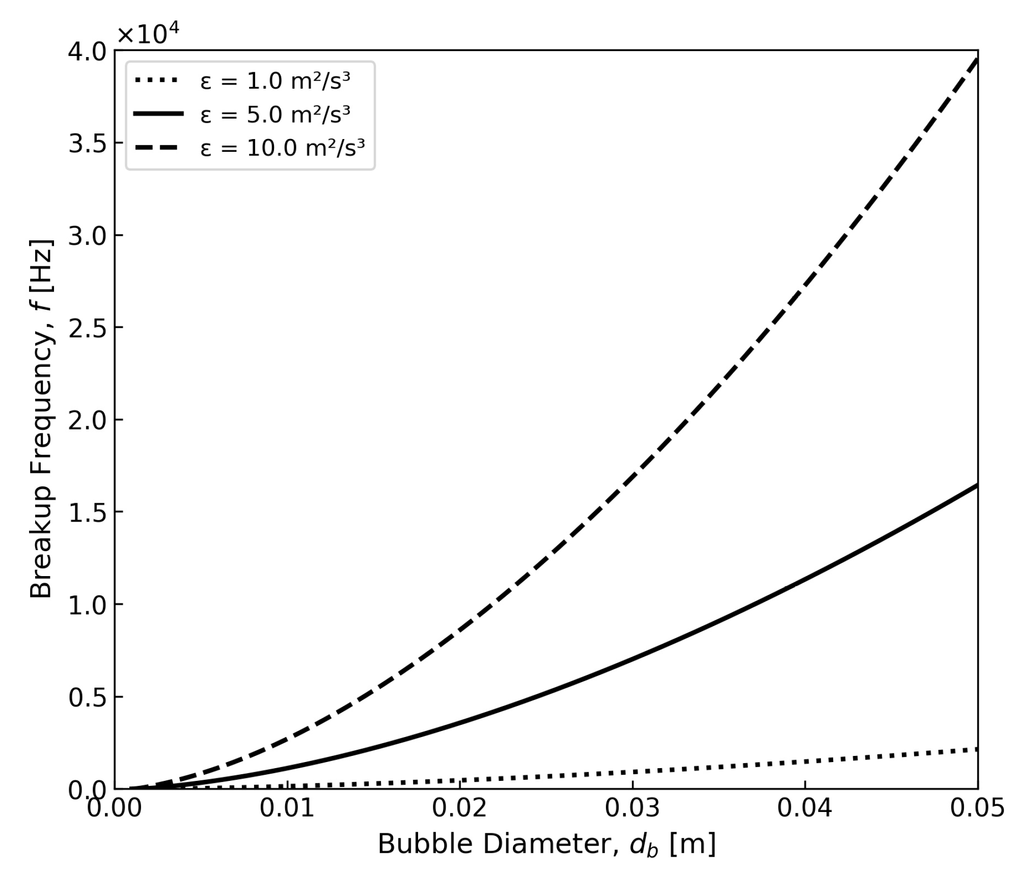
Figure 2 illustrates the variation in bubble breakup frequency with bubble diameter and turbulent dissipation rate, as predicted by the model of Lehr et al. [28]. The results show that the breakup frequency increases significantly with both the bubble diameter and the turbulent energy dissipation rate (ε). For small bubbles (<0.01 m), the breakup frequency remains relatively low, while for larger bubbles the breakup frequency rises steeply, especially under higher turbulence intensities (ε = 5.0 and 10.0 m2/s3). As shown in Figure 3, Lehr et al.’s daughter bubble volume distribution model is characterized by the fact that, as bubble size increases, the turbulent kinetic energy in the surrounding flow field grows, and f b v more readily develops a maximum at an offset of 0.5—i.e., it tends toward unequal size breakup. Conversely, smaller bubbles reside in regions of lower turbulent kinetic energy, and the function f b v more readily exhibits a peak at 0.5—i.e., the breakup tends toward two daughter bubbles of nearly equal volume.

3. Simulation Conditions and Procedure

The liquid–gas two-phase flow in a steel continuous casting mold was simulated using the three-dimensional Euler–Lagrange method. For subsequent comparison and validation, the present simulation conditions and parameters are based on the water model experiments of Wu et al. [7,12,29]. These parameters, for both the water model and the prototype, are listed in Table 2 to ensure consistency and allow for a direct comparison with their experiment.
The Euler framework for water was solved in commercial CFD software, Ansys Fluent version 18.1 [30]. The Lagrange framework for bubbles was solved in an in-house code. The interaction data were transmitted synchronously via a user-defined function (UDF) at each computational time step. Specifically, once the computational cell containing a given bubble is identified, the local fluid velocity and other pertinent grid data are retrieved via a user-defined function (UDF), and these values are then used to compute the bubble’ s motion, coalescence, and breakup. At the same time, the effect of bubbles on other phases can be transmitted through the user-defined source term. In Fluent, double precision was used, and the convergence residual was set to 0.0001. The simulation area was discretized into 253,756 grid cells, and further grid refinement did not result in significant changes to the simulation results. After repeated tests and comprehensive consideration of the computational cost and calculation accuracy, the timesteps of the Euler and Lagrange phases were selected as 0.0005 and 0.0001 s, respectively.
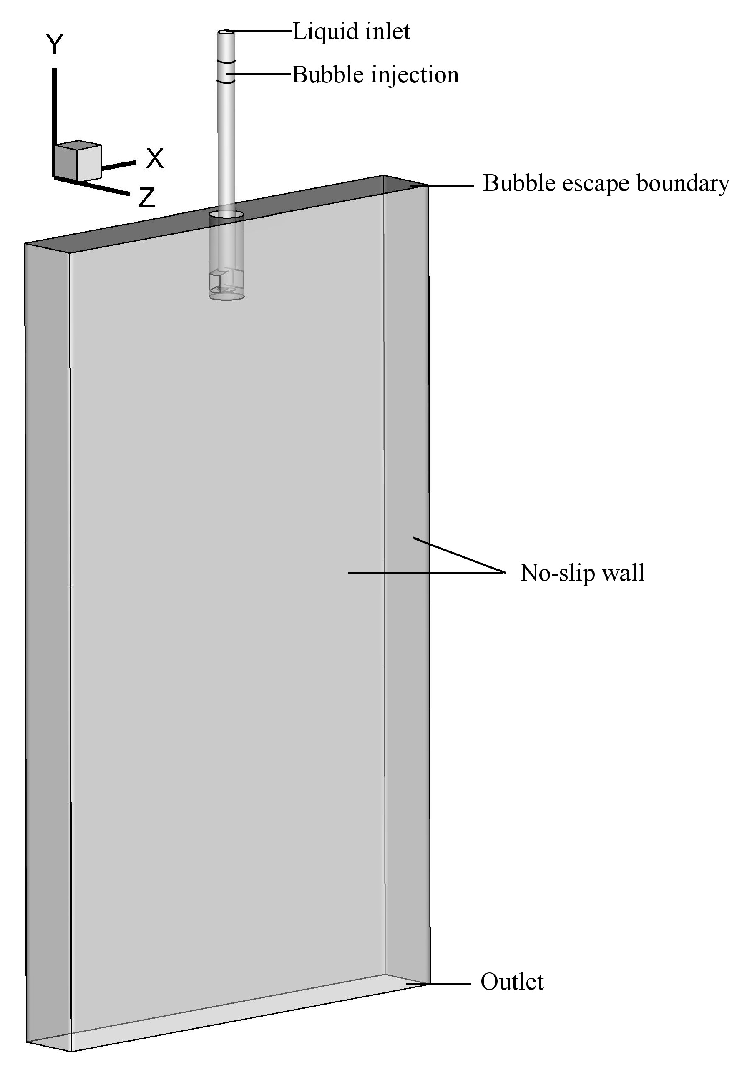
The boundary conditions for the liquid phase are configured as follows. As illustrated in Figure 4, the liquid inlet is specified as a mass flow inlet. Bubbles are introduced from the inner wall of the submerged entry nozzle. The side walls of the water model and the nozzle wall are set to no slip conditions for the liquid and rebound conditions for the bubbles. The top surface serves as the outlet for the gas phase and as a free slip wall for the liquid. The initial diameter of the injected bubbles is 0.893 mm, in accordance with Wu et al. [29].

4. Results and Discussion

To study the importance of bubble swarm correction model and their effect on the results, simulations and analyses were performed for the three cases listed in Table 3 at water flow rates of 900 L/h. The aim was to gain a deeper understanding of how the bubble swarm correction model influenced the outcomes of the simulations and whether it was necessary to incorporate this model for accurate predictions.
Case 1 served as a baseline to compare against the other two cases, where no bubble swarm correction was applied. Case 2 employed the model by Garnier et al. [11], while case 3 employed the model by Roghair et al. [19].

4.1. Bubble Distribution and Trajectory

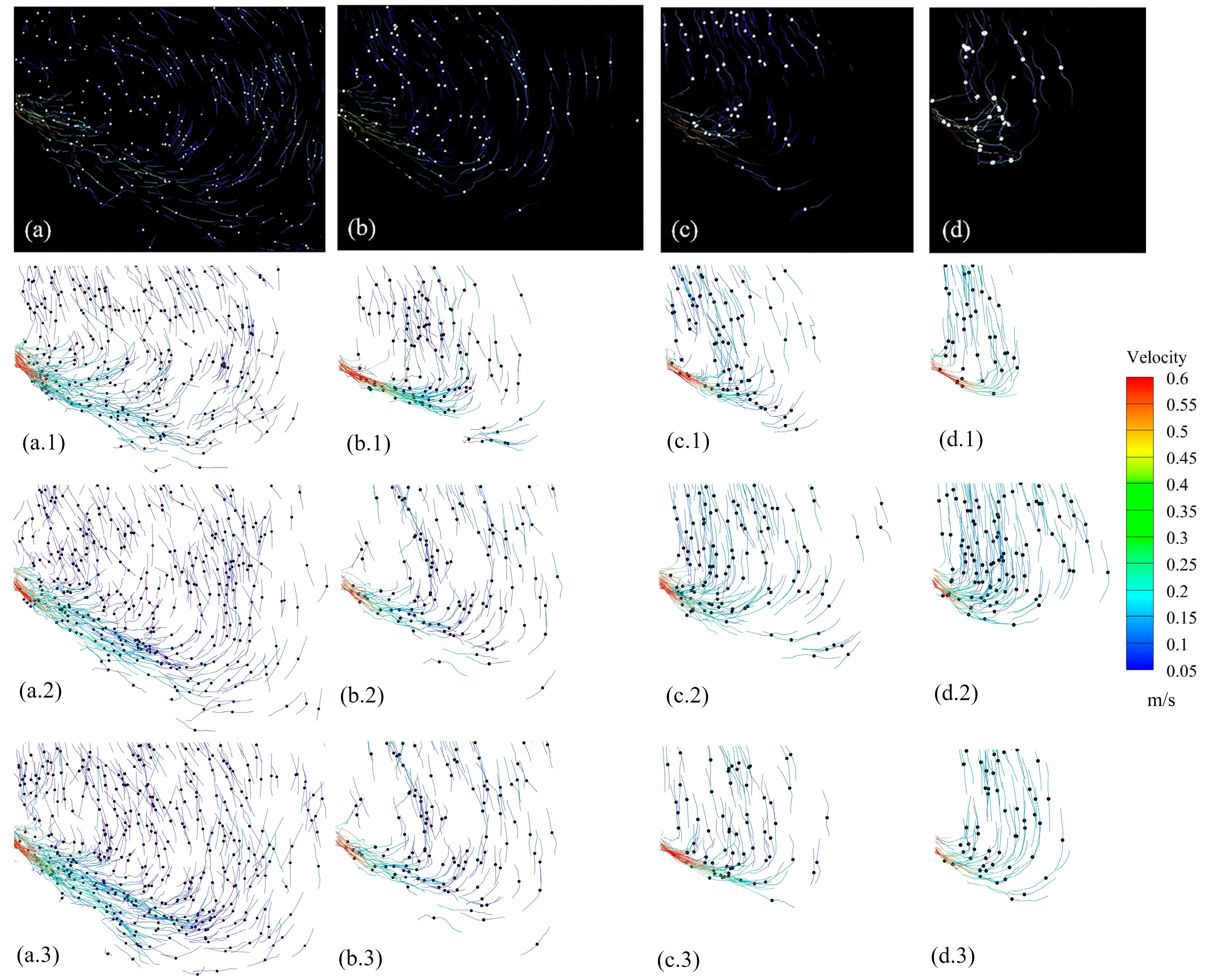
Figure 5 presents the bubble trajectories for different bubble sizes under a gas flow rate of 400 mL⋅min−1. The first row displays the experimental results, while the subsequent rows correspond to simulations of Case 1 (no swarm drag correction), Case 2 (Garnier et al. [11]), and Case 3 (Roghair et al. [19]). These cases represent different approaches to correcting the drag coefficient based on bubble swarm effects. Figure 6 provides a statistical analysis of the Hausdorff distance error between the simulated and experimental bubble trajectories from Figure 5, focusing on both grid and time step independence. For each condition in panels (a) and (b), five independent simulations were performed to account for potential variability in the results. The mean values are plotted, and the corresponding standard deviations are all below 5% of the mean, indicating a high degree of repeatability. Panel (a) shows the effect of cell number on Hausdorff distance, with a fixed time step of 0.0001 s, while Panel (b) illustrates the impact of time step variation, keeping the grid number constant at 253,756. This analysis underscores the stability and convergence of the simulation results as the grid resolution and time steps are refined, confirming that further refinement does not significantly alter the results. Therefore, Figure 6 serves as a statistical validation of the bubble trajectory simulations presented in Figure 5.
The comparison of the bubble trajectory simulations across different cases highlights the impact of drag forces on bubble behavior, specifically with respect to their horizontal displacement. As drag forces increase, bubbles experience greater resistance to upward movement, leading to a reduced rising velocity and a prolonged time for lateral displacement, along with a higher lateral displacement velocity under the impact of the main steel flow. This behavior is the most apparent in Case 3, which incorporates the Roghair et al. bubble swarm drag correction model. This model provides the most accurate prediction of bubble trajectories, particularly for larger bubbles that experience less drag. In contrast, Case 2, which uses the Garnier model, underestimates the drag correction for larger bubbles and overestimates it for smaller bubbles, leading to discrepancies in the predicted bubble paths. In Case 1, without any drag correction, the simulations fail to capture the full extent of drag effects, resulting in the largest deviations from the experimental measurements. As a result, the driving effect of the liquid jet at the nozzle outlet is minimal, the horizontal travel distance of the bubbles is the shortest and the deviation from the experimental data is the greatest. Specifically, in column d of Figure 5, focusing on bubbles larger than 2.5 mm, Case 3 matches the experimental results very well in terms of travel distance under impingement, whereas in Case 2 the large bubbles are carried slightly farther by the liquid jet than observed in the experiments.
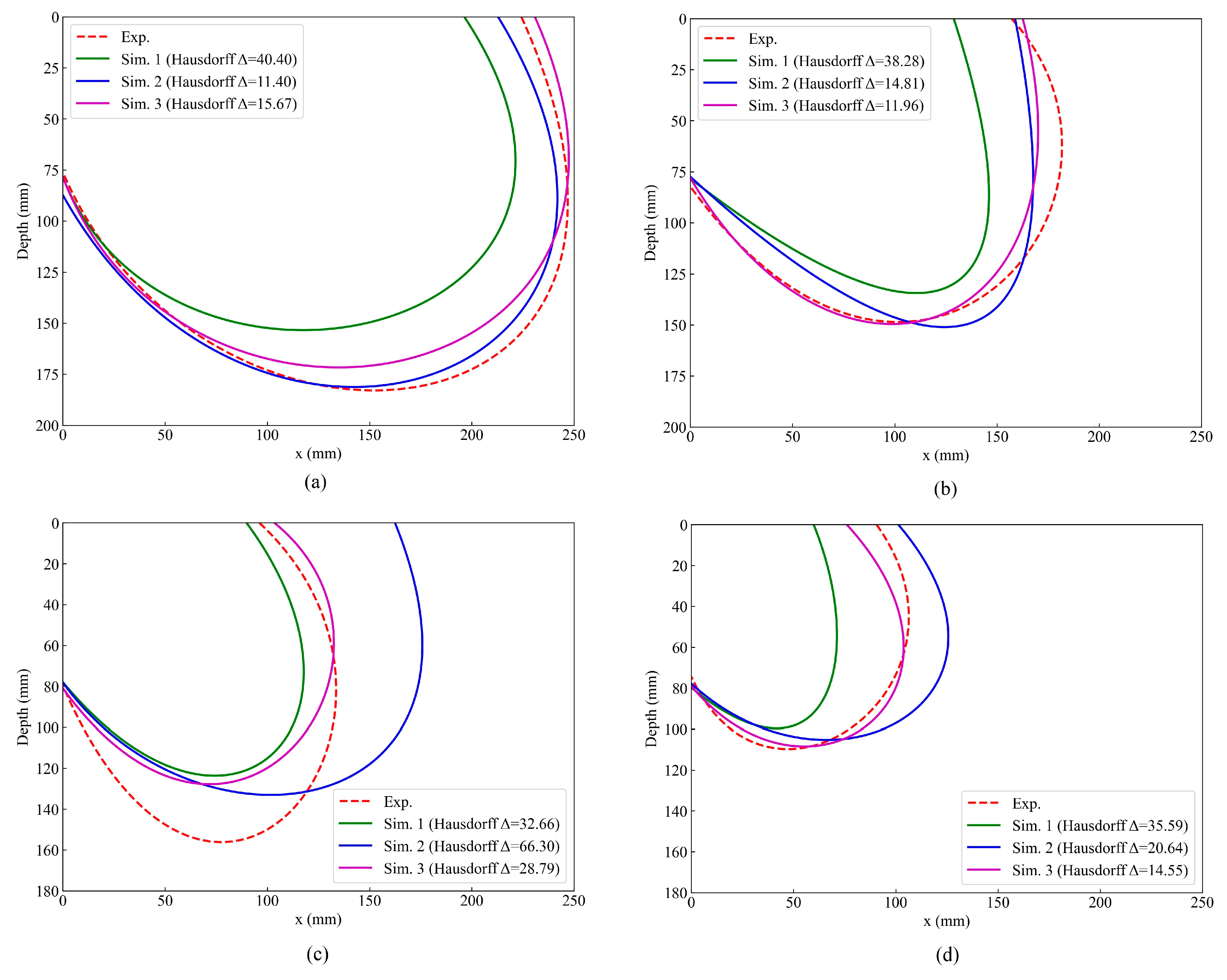
Figure 7 enclosing trajectories of bubbles over a 60 s period at a gas flow rate of 400 mL⋅min−1. The bounding lines in this figure were obtained using a least-squares method, with an added tolerance to ensure that only the main bubble trajectories were enclosed, avoiding the influence of non-primary gas flows. Unlike Figure 5, which shows bubble trajectories at a specific moment, this figure presents the statistical results over the entire 60 s period. The analysis revealed that extending the statistical time beyond 60 s had minimal impact on the results, confirming the robustness of the findings. Deviations from the experimental data are quantified using Hausdorff distance, a metric that measures the maximum distance between points on two sets (in this case, the predicted and experimental bubble trajectories). Smaller values of Hausdorff distance indicate better agreement between the simulation results and the experimental data. When comparing the performance of the models across all four plots, Case 3 (Roghair model) shows the smallest Hausdorff distance, indicating the best alignment with the experimental data. Furthermore, Case 3 exhibited the greatest improvement in reducing the error compared to Case 1 (no correction model). On average, Case 3 reduced the error by 51.7%, which is significantly better than the 23.0% improvement achieved by Case 2 (Garnier model). This further confirms the superior performance of the Roghair model in capturing the bubble flow behavior and enhancing the accuracy of the simulation results.
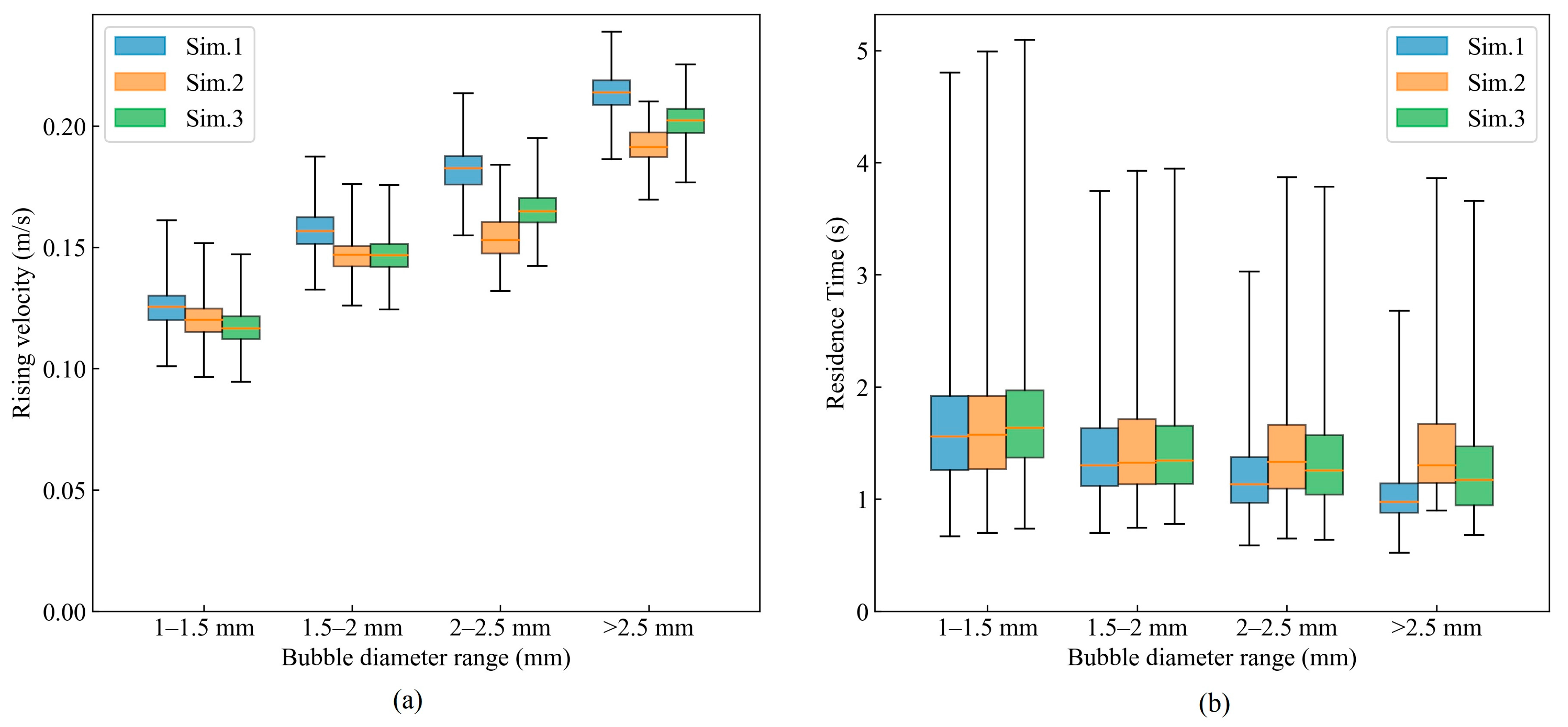
As shown in Figure 8a, across all simulations, the median rising velocity increases with bubble diameter, as expected from buoyancy. Introducing swarm-drag corrections lowers the rising velocity compared with Sim. 1 (no correction). The extent of the reduction depends on the correlation: for small bubbles (1.0–1.5 mm), Sim. 3 (Roghair et al. [19]) yields slightly lower velocities than Sim. 2 (Garnier et al. [11]), consistent with a larger correction factor f(α) predicted by Roghair et al. for small diameters. In contrast, for larger bubbles (2.0–2.5 mm and >2.5 mm), Sim. 2 produces the lower rising velocity, which aligns with Garnier et al. [11] giving a larger f(α) than Roghair et al. [19] at these diameters and typical local volume fractions. The 1.5–2.0 mm class shows intermediate behavior with only a modest difference between the two correlations. As shown in Figure 8b, the residence time exhibits the opposite trend to rising velocity. Both correlations increase the residence time relative to Sim.1, reflecting the reduced slip caused by the higher effective drag. Consistent with the rising velocity trends, Sim. 3 tends to give longer residence times for 1.0–1.5 mm bubbles, whereas Sim. 2 yields longer residence time for 2.0–2.5 mm and >2.5 mm bubbles.
In Figure 8, the separation among Sim. 1–3 is more pronounced for the two largest classes (2.0–2.5 mm and >2.5 mm). Larger bubbles mainly rise within the near-nozzle region where the gas holdup is highest; because the swarm-drag amplification increases with the local volume fraction, the effective drag is strengthened there, leading to a greater reduction in rising velocity and a longer residence time than for the smaller-diameter classes. The size-dependent trends in Figure 8 rationalize the trajectory differences reported in Figure 5. Whenever a swarm-drag correlation yields a stronger increase in the effective drag for a given diameter class, the slip and rise velocities are reduced and the bubble residence time is extended. The longer residence near the jet–impingement region exposes bubbles to the horizontal steel stream for a greater duration, which explains the observed changes in travel distance in Figure 5. Conversely, when the swarm-drag amplification is weaker, bubbles exit the jet sooner, producing shorter paths and larger mismatches with the measured trajectories.
Figure 9 shows the bubble size distributions along three horizontal lines at depths of 3 mm, 27 mm and 51 mm from the surface. The experimental data are taken from the 1/4-scale water model study of Wu et al. [12], in which bubble sizes were measured from 500 consecutive frames recorded at 1000 fps, averaged over 70 subregions in the region of interest, ensuring high statistical robustness and minimizing random error. Given the large sampling size and rigorous averaging procedure in the experiments, these data have high repeatability and provide a reliable basis for quantitative model validation. It can be seen that all three cases predict a decrease in bubble size with increasing distance x from the nozzle. Among them, Case 3, which employs the Roghair model, achieves the best overall agreement with the experimental data, followed by Case 2 using the Garnier model. In Case 1, where no swarm drag correction is applied, the drag coefficient is underestimated, resulting in weaker entrainment by the steel flow, reduced horizontal displacement and the largest deviation from the experimental measurements. Relative to Case 1, Case 2 using the Garnier model carries larger bubbles farther but still exhibits noticeable discrepancies with the data. The superior performance of the Roghair model likely arises from its more accurate treatment of bubble swarm effects on drag. This finding underscores the importance of selecting an appropriate swarm correction model to achieve reliable predictions of bubble behavior in metallurgical processes.

4.2. The Influence of Drag Force on Liquid Phase Flow Field

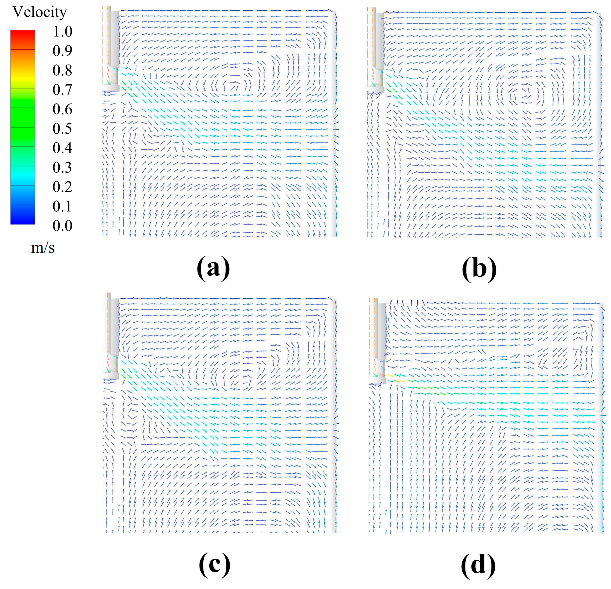
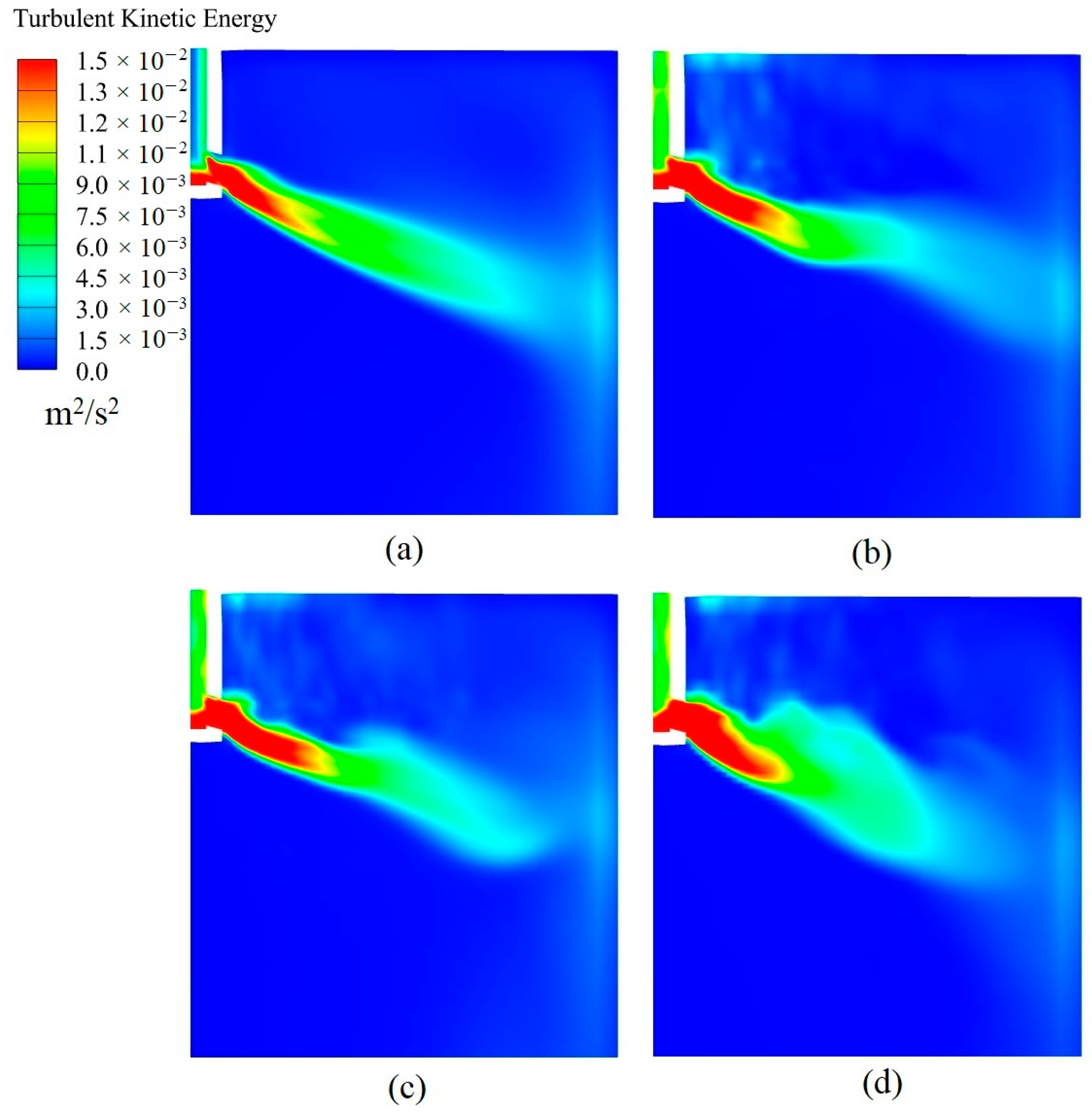
Figure 10 compares the liquid-phase velocity vectors under four operating conditions, and Figure 11 shows the corresponding turbulent-kinetic-energy (TKE) contours on the same mid-plane. Without bubble injection (Figure 10a and Figure 11a), the flow exhibits the classic double-roll circulation generated by the impingement of the jet on the narrow face, while the TKE is confined to the jet shear layer and the impingement zone. After bubbles are introduced (Figure 10b–d and Figure 11b–d), pronounced disturbances appear and the high-TKE region expands both along the jet and toward the upper recirculation cell, indicating enhanced momentum exchange between phases. These disturbances originate from the interaction between the bubbles and the surrounding fluid, in particular the drag exerted by the liquid on the bubbles and the corresponding reaction force. To quantify this effect, we computed the volume-averaged turbulent kinetic energy (TKE) within the 0–200 mm depth shown in Figure 10 and Figure 11. In the absence of bubble injection situation, the TKE is 0.0013 m2/s2; it rises to 0.0015 m2/s2 in Case 1, 0.0025 m2/s2 in Case 2, and 0.0027 m2/s2 in Case 3. This indicates that bubble injection generates extra flow disturbances in the continuous casting mold, and that simulations using drag-correction models predict stronger disturbances than those without correction. Spatially, Figure 11 shows that the additional TKE generated with drag-correction models is concentrated in the jet shear layer and spreads more broadly into the upper roll, consistent with the stronger fluctuations and larger eddies visible in the velocity vectors of Figure 10.
In Case 1, without any swarm drag correction (Figure 10b and Figure 11b), the flow field shows only moderate disturbance near the injection region. Because the drag coefficient on the bubbles is underestimated, the overall flow pattern remains largely unchanged apart from localized turbulence. By contrast, Case 2, which applies the Garnier model (Figure 10c and Figure 11c), produces noticeably stronger disturbances. The drag corrected for bubble–bubble interactions drives more vigorous liquid motion and generates a more complex flow structure around the nozzle compared with Case 1. In Case 3, employing the Roghair model (Figure 10d and Figure 11d), yields the most significant alteration of the flow field. The drag, fully corrected for swarm effects, induces intense disruption of the liquid stream. The bubbles’ entrainment of the steel flow produces a clearly visible lifting effect.

5. Conclusions

This study systematically investigates the impact of a bubble swarm correction model on the simulation of bubble behavior within a continuous casting mold. By comparing simulations with and without bubble swarm correction, it is evident that incorporating such a model enhances predictive accuracy. In particular, the model proposed by Roghair et al. yields the best overall performance under the specific conditions investigated in this study, including bubble sizes under 3 mm and gas flow rates up to 850 mL/min, exhibiting excellent agreement with experimental measurements in terms of bubble trajectories, size distributions and their influence on the liquid-phase flow field.
Analysis of bubble trajectories shows that the Roghair model accurately captures the decrease in bubble size with increasing distance from the submerged entry nozzle. Moreover, this model reliably predicts the horizontal displacement of bubbles under the action of drag imposed by the steel flow. The analysis of Hausdorff distances in the trajectory predictions confirms that the Roghair model achieves the smallest residuals in the overall trajectory predictions, with an average error reduction of 51.7%, indicating the best agreement with experimental data. This underscores the significant advantage of the Roghair model in accurately capturing bubble dynamics and improving the overall accuracy of the trajectory predictions.
With respect to bubble size distribution, the Roghair model again demonstrates close alignment with experimental observations across different depths and gas flow rates. This accuracy underlines the importance of accounting for bubble swarm effects when modeling bubble dynamics in metallurgical processes.
The investigation of drag effects on the liquid flow field further underscores the significance of the bubble swarm correction. The introduction of bubbles causes substantial disturbances in the liquid flow, and the intensity of these disturbances increases with the complexity of the correction model employed. Notably, the Roghair model produces the most pronounced flow field modifications, with the main steel stream carried by the bubbles exhibiting a marked lifting effect.
In summary, the results of this study emphasize the critical role of bubble swarm correction models in accurately simulating bubble behavior and its interaction with the liquid phase. For the specific conditions of continuous casting molds, our findings clearly indicate that the model of Roghair et al. is the optimal choice for achieving precise predictions. While other models may have their merits in different scenarios, the Roghair et al. model demonstrated superior accuracy for this metallurgical application.

Author Contributions

Conceptualization, Q.L., Z.L. and Z.Z.; methodology, Q.L.; software, Q.L.; validation, Q.L., Z.L. and H.L.; formal analysis, Q.L.; investigation, Q.L.; resources, Q.L.; data curation, Q.L. and Y.Z.; writing—original draft preparation, Q.L.; writing—review and editing, Z.L., Y.Z., Z.Z. and H.L.; visualization, Q.L.; supervision, Z.L. and Y.Z.; project administration, Z.L.; funding acquisition, H.L. All authors have read and agreed to the published version of the manuscript.

Funding

Financial support was provided by the National Key R&D Program of China (No. 2023YFB4204000).

Data Availability Statement

The original contributions presented in this study are included in the article. Further inquiries can be directed to the corresponding authors.

Conflicts of Interest

Author Yongjie Zhang was employed by the company Energy and Environment Research Institute R & D Center, Baosteel Group Corporation. The remaining authors declare that the research was conducted in the absence of any commercial or financial relationships that could be construed as a potential conflict of interest.

Abbreviations

The following abbreviations are used in this manuscript:
SENSubmerged Entry Nozzle
PBMPopulation Balance Model
DNSDirect Numerical Simulation

References

  1. Deng, X.; Ji, C.; Zhu, G.; Liu, Q.; Huang, F.; Tian, Z.; Wang, X. Quantitative evaluations of surface cleanliness in IF steel slabs at unsteady casting. Metall. Mater. Trans. B 2019, 50, 1974–1987. [Google Scholar] [CrossRef]
  2. Miki, Y.; Takeuchi, S. Internal defects of continuous casting slabs caused by asymmetric unbalanced steel flow in mold. ISIJ Int. 2003, 43, 1548–1555. [Google Scholar] [CrossRef]
  3. Jin, K.; Thomas, B.G.; Ruan, X.M. Modeling and measurements of multiphase flow and bubble entrapment in steel continuous casting. Metall. Mater. Trans. B 2015, 47, 548–565. [Google Scholar] [CrossRef]
  4. Zhang, T.; Luo, Z.G.; Liu, C.L.; Zhou, H.; Zou, Z.S. A mathematical model considering the interaction of bubbles in continuous casting mold of steel. Powder Technol. 2015, 273, 154–164. [Google Scholar] [CrossRef]
  5. Yang, W.; Luo, Z.; Gu, Y.; Liu, Z.; Zou, Z. Simulation of bubbles behavior in steel continuous casting mold using an Euler-Lagrange framework with modified bubble coalescence and breakup models. Powder Technol. 2020, 361, 769–781. [Google Scholar] [CrossRef]
  6. Liu, Z.Q.; Qi, F.S.; Li, B.K.; Cheung, S.C.P. Modeling of bubble behaviors and size distribution in a slab continuous casting mold. Int. J. Multiph. Flow 2016, 79, 190–201. [Google Scholar] [CrossRef]
  7. Wu, Y.; Liu, Z.; Li, B.; Xiao, L.; Gan, Y. Numerical simulation of multi-size bubbly flow in a continuous casting mold using an inhomogeneous multiple size group model. Powder Technol. 2022, 402, 117368. [Google Scholar] [CrossRef]
  8. Dijkhuizen, W.; Roghair, I.; Van Sint Annaland, M.; Kuipers, J. Numerical derivation of the drag force coefficient in bubble swarms using a front tracking model. In Proceedings of the 6th International Conference on CFD in the Oil and Gas, Metallurgical and Process Industries, Trondheim, Norway, 10–12 June 2008. [Google Scholar]
  9. Roghair, I.; Baltussen, M.W.; Van Sint Annaland, M.; Kuipers, J.A.M. Direct Numerical Simulations of the drag force of bi-disperse bubble swarms. Chem. Eng. Sci. 2013, 95, 48–53. [Google Scholar] [CrossRef]
  10. Simonnet, M.; Gentric, C.; Olmos, E.; Midoux, N. Experimental determination of the drag coefficient in a swarm of bubbles. Chem. Eng. Sci. 2007, 62, 858–866. [Google Scholar] [CrossRef]
  11. Garnier, C.; Lance, M.; Marié, J.L. Measurement of local flow characteristics in buoyancy-driven bubbly flow at high void fraction. Exp. Therm. Fluid Sci. 2002, 26, 811–815. [Google Scholar] [CrossRef]
  12. Wu, Y.; Liu, Z.; Wang, F.; Li, B.; Gan, Y. Experimental investigation of trajectories, velocities and size distributions of bubbles in a continuous-casting mold. Powder Technol. 2021, 387, 325–335. [Google Scholar] [CrossRef]
  13. Yang, G.; Zhang, H.; Luo, J.; Wang, T. Drag force of bubble swarms and numerical simulations of a bubble column with a CFD-PBM coupled model. Chem. Eng. Sci. 2018, 192, 714–724. [Google Scholar] [CrossRef]
  14. Yan, P.; Jin, H.; He, G.; Guo, X.; Ma, L.; Yang, S.; Zhang, R. CFD simulation of hydrodynamics in a high-pressure bubble column using three optimized drag models of bubble swarm. Chem. Eng. Sci. 2019, 199, 137–155. [Google Scholar] [CrossRef]
  15. Tomiyama, A. Struggle with Computational Bubble Dynamics. Multiph. Sci. Technol. 1998, 10, 369–405. [Google Scholar] [CrossRef]
  16. Zhang, D.; Deen, N.G.; Kuipers, J.A.M. Numerical simulation of the dynamic flow behavior in a bubble column: A study of closures for turbulence and interface forces. Chem. Eng. Sci. 2006, 61, 7593–7608. [Google Scholar] [CrossRef]
  17. Troshko, A.; Hassan, Y. A two-equation turbulence model of turbulent bubbly flows. Int. J. Multiph. Flow 2001, 27, 1965–2000. [Google Scholar] [CrossRef]
  18. Zenit, R.; Koch, D.L.; Sangani, A.S. Measurements of the average properties of a suspension of bubbles rising in a vertical channel. J. Fluid Mech. 2001, 429, 307–342. [Google Scholar] [CrossRef]
  19. Roghair, I.; Van Sint Annaland, M.; Kuipers, H.J.A.M. Drag force and clustering in bubble swarms. AlChE J. 2012, 59, 1791–1800. [Google Scholar] [CrossRef]
  20. Ishii, M.; Zuber, N. Drag coefficient and relative velocity in bubbly, droplet or particulate flows. AlChE J. 1979, 25, 843–855. [Google Scholar] [CrossRef]
  21. Spelt, P.; Biesheuvel, A. On the motion of gas bubbles in homogeneous isotropic turbulence. J. Fluid Mech. 1997, 336, 221–244. [Google Scholar] [CrossRef]
  22. Lockett, M.J.; Kirkpatrick, R.D. Ideal bubbly flow and actual flow in bubble columns. Trans. Inst. Chem. Eng. 1975, 53, 267–273. [Google Scholar]
  23. Bai, H.; Thomas, B.G. Bubble formation during horizontal gas injection into downward-flowing liquid. Metall. Mater. Trans. B 2001, 32, 1143–1159. [Google Scholar] [CrossRef]
  24. Planquart, P.; Dehaeck, S.; Buchlin, J.M.; Riethmuller, M. Experimental Investigation of Bubbly Flow, Annular Flow and Transition in a Downward Cocurrent Two-Phase Flow. In Proceedings of the Icmf, Yokohama, Japan, 30 May–4 June 2004. [Google Scholar]
  25. Chen, Y.; Wang, L.; Chang, H.; Zhang, Q. A Review of Drag Coefficient Models in Gas-Liquid Two-Phase Flow. ChemBioEng Rev. 2023, 10, 311–325. [Google Scholar] [CrossRef]
  26. Chesters, A.K.; Hofman, G. Bubble coalescence in pure liquids. Appl. Sci. Res. 1982, 38, 353–361. [Google Scholar] [CrossRef]
  27. Duineveld, P. Bouncing and coalescence of bubble pairs rising at high Reynolds number in pure water or aqueous surfactant solutions. Appl. Sci. Res. 1998, 58, 409–439. [Google Scholar] [CrossRef]
  28. Lehr, F.; Millies, M.; Mewes, D. Bubble-Size distributions and flow fields in bubble columns. AlChE J. 2002, 48, 2426–2443. [Google Scholar] [CrossRef]
  29. Wu, Y.; Liu, Z.; Li, B.; Gan, Y. Numerical simulation of multi-size bubbly flow in a continuous casting mold using population balance model. Powder Technol. 2022, 396, 224–240. [Google Scholar] [CrossRef]
  30. ANSYS Inc. ANSYS Fluent Theory Guide, Release 18.1; ANSYS Inc.: Canonsburg, PA, USA, 2017. [Google Scholar]
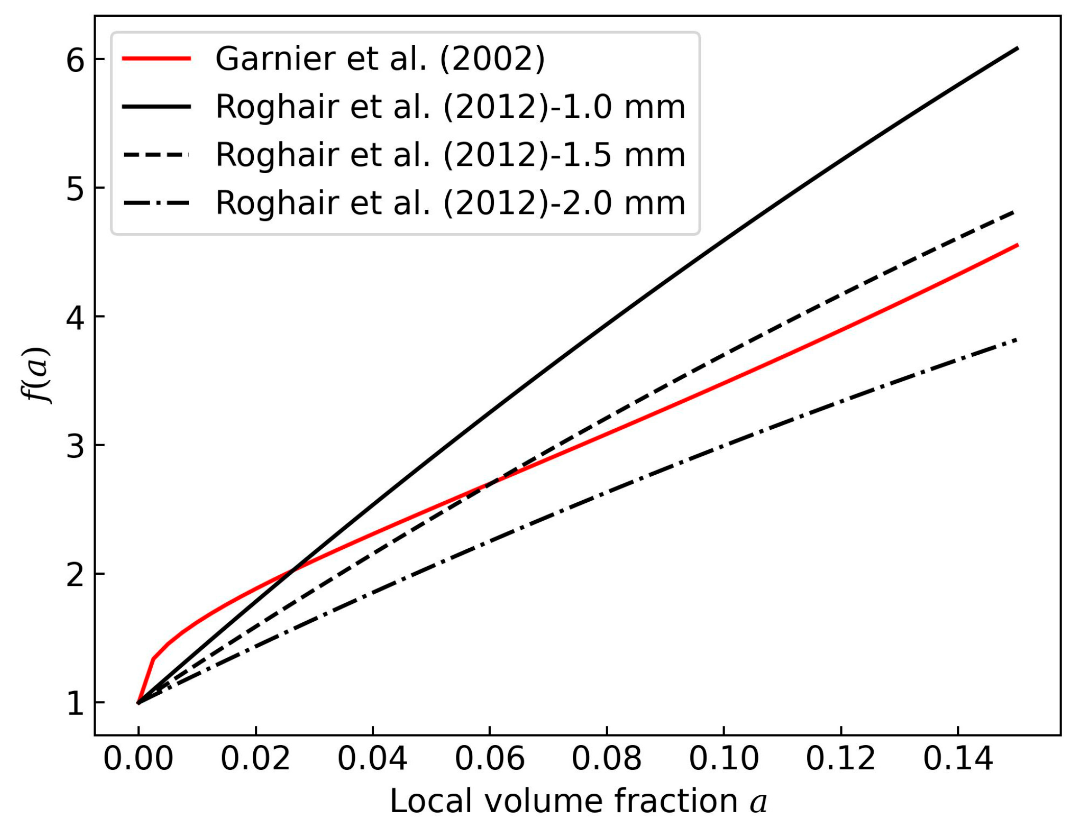
Figure 1. The relationship between the bubble swarm drag correction coefficient and the gas phase volume fraction. Curves were computed and plotted by the authors from the correlations adapted from Refs. [11,19].
Metals 15 00952 g001
Figure 2. Variation in bubble breakup frequency with turbulent dissipation rate and bubble diameter.
Metals 15 00952 g002
Figure 3. Probability distribution of daughter bubble volumes after binary breakup.
Metals 15 00952 g003
Figure 4. Schematic diagram of the geometry and boundary of the simulation area.
Metals 15 00952 g004
Figure 5. Snapshot of trajectories of bubbles within diameter range of (a) 1–1.5 mm, (b) 1.5–2 mm, (c) 2–2.5 mm, (d) above 2.5 mm at gas flow rate of 400 mL·min−1. The first row shows the experimental results reprinted with permission from ref. [12]. Copyright 2021, Elsevier. and (x.1), (x.2), and (x.3) correspond to Case 1, Case 2, and Case 3, respectively. In detail, (a.1) 1–1.5 mm bubbles in Case 1; (a.2) 1–1.5 mm bubbles in Case 2; (a.3) 1–1.5 mm bubbles in Case 3. Similarly, (b.1) 1.5–2 mm bubbles in Case 1; (b.2) 1.5–2 mm bubbles in Case 2; (b.3) 1.5–2 mm bubbles in Case 3. (c.1) 2–2.5 mm bubbles in Case 1; (c.2) 2–2.5 mm bubbles in Case 2; (c.3) 2–2.5 mm bubbles in Case 3. (d.1) Above 2.5 mm bubbles in Case 1; (d.2) Above 2.5 mm bubbles in Case 2; (d.3) Above 2.5 mm bubbles in Case 3.
Metals 15 00952 g005
Figure 6. Grid and time step independence analysis based on Hausdorff distance error between simulation and experimental trajectories. (a) The effect of cell number on Hausdorff distance, with a fixed time step of 0.0001 s. (b) The effect of time step on Hausdorff distance, with a fixed grid number of 253,756.
Metals 15 00952 g006
Figure 7. Enclosing trajectories of bubbles for different diameter ranges at a gas flow rate of 400 mL⋅min−1. The curves represent the bounding lines of the bubble trajectories for (a) 1–1.5 mm, (b) 1.5–2 mm, (c) 2–2.5 mm, and (d) above 2.5 mm.
Metals 15 00952 g007
Figure 8. Effect of bubble-swarm drag corrections on (a) rising velocity relative to water and (b) residence time in mold for different bubble-diameter classes at a gas flow rate of 400 mL⋅min−1. Results are shown for Sim. 1 (no correction), Sim. 2 (using the Garnier et al. (Adapted from Ref. [11]) model), and Sim. 3 (using the Roghair et al. (Adapted from Ref. [19]) model). Boxes denote the interquartile range with the median as a central line; whiskers indicate the overall spread of the samples. All data are based on the statistics of bubbles that rose to the free surface during a 5 min simulation window.
Metals 15 00952 g008
Figure 9. Bubble size distribution at depths of (a) 3, (b) 27, and (c) 51 mm at gas flow rate of 550 mL/min.
Metals 15 00952 g009
Figure 10. Flow field (a) No bubble injection, (b) Case 1 (no swarm-drag correction), (c) Case 2 (using the Garnier et al. (Adapted from Ref. [11]) model), (d) Case 3 (using the Roghair et al. (Adapted from Ref. [19]) model).
Metals 15 00952 g010
Figure 11. Contours of turbulence kinetic energy (a) No bubble injection, (b) Case 1 (no swarm-drag correction), (c) Case 2 (using the Garnier et al. (Adapted from Ref. [11]) model), (d) Case 3 (using the Roghair et al. (Adapted from Ref. [19]) model).
Metals 15 00952 g011
Table 1. Applicability ranges of the Garnier and Roghair bubble-swarming correction models.
ParametersGarnier et al. [11]Roghair et al. [19]
Void fraction0–0.30–0.4
Bubble Reynolds number300–500No explicit limit
Eotvos numbersNo explicit limit0.13 to 4.9
Bubble diameter (mm)1.0–5.51.0–6.0
Table 2. Geometrical and process parameters in water model and prototype. Reprinted from Ref. [12].
ParameterWater ModelPrototype
Mold width × thickness (mm)550 × 752200 × 300
Mold/strand height (mm)900Open bottom
Diameter of SEN (mm)2080
Length of SEN (mm)3051220
Exit angle of nozzle (degree)1515
SEN port height × width (mm)20 × 17.580 × 70
Submergence depth of SEN (mm)75300
Density of liquid phase (kg/m3)10007020
Density of gas phase (kg/m3)1.1380.56
Viscosity of liquid phase (N·s/m2)0.0010.0056
Volume flow rate of liquid phase (L/h)700–110022,400–35,200
Volume flow rate of gas phase (mL/min)400–8508000–17,000
Interfacial tension (N/m)0.0721.5
Table 3. Summary of simulation cases with different bubble swarm drag correction models.
Case Bubble Swarm Correction Model
1No correction
2Garnier et al. (2002) [11], Equation (13)
3Roghair et al. (2012) [19], Equation (14)
Disclaimer/Publisher’s Note: The statements, opinions and data contained in all publications are solely those of the individual author(s) and contributor(s) and not of MDPI and/or the editor(s). MDPI and/or the editor(s) disclaim responsibility for any injury to people or property resulting from any ideas, methods, instructions or products referred to in the content.