Article

Towards a Global Constitutive Formulation for Modeling the Hot Working Behavior of Low-Carbon Steels

by
Unai Mayo
1,2,*,
Sergio Fernandez-Sanchez
1,2,
Isabel Gutierrez
1,2,
Denis Jorge-Badiola
1,2 and
Amaia Iza-Mendia
1,2
1
Ceit-Member of Basque Research & Technology Alliance (BRTA), Donostia-San Sebastián 20018, Gipuzkoa, Spain
2
Mechanical and Materials Engineering Department, Tecnun-Universidad de Navarra, Donostia-San Sebastián 20018, Gipuzkoa, Spain
*
Author to whom correspondence should be addressed.
Metals 2025, 15(9), 1044; https://doi.org/10.3390/met15091044
Submission received: 3 July 2025 / Revised: 4 September 2025 / Accepted: 10 September 2025 / Published: 19 September 2025

Abstract

The current study explores the applicability of a single constitutive equation, based on the Arrhenius hyperbolic sine model, to a wide range of chemical compositions and test conditions by using a unique approximation. To address this challenge, a mixed model is proposed, integrating a physical model with phenomenological expressions to capture the strain and strain rate hardening, forming temperature, dynamic recovery (DRV) and dynamic recrystallization (DRX). The investigation combines high-temperature mechanical testing with modeling in order to understand the hot deformation mechanisms. Hot torsion tests were conducted on ten different low-carbon steels with distinct microalloying additions to capture their responses under diverse initial austenite grain sizes, deformation temperatures and strain rate conditions (d0 = 22–850 µm, T = 800–1200 °C and ε ˙ = 0.1–10 s−1). The developed constitutive equation has resulted in a robust expression that effectively simulates the hot behavior of various alloys across a wide range of conditions. The application of an optimization tool has significantly reduced the need for adjustments across different alloys, temperatures and strain rates, showcasing its versatility and effectiveness in predicting the flow behavior in a variety of scenarios with excellent accuracy. Moreover, the model has been validated with experimental torsion data from the literature, enhancing the applicability of the developed expression to a broader spectrum of chemical compositions.

1. Introduction

Together with the digitalization of industrial plants, material forming simulation models are gaining growing importance due to their effective role in the control of manufacturing processes [1,2,3,4]. It is known that the optimization of the final mechanical properties is strictly related to control over the process parameters, with the modeling of the flow behavior of the material being a relevant input to achieving this goal. The flow response at high temperatures is difficult to describe by means of a simple expression, as many interconnected metallurgical phenomena take place during hot deformation: strain hardening, dynamic recovery (DRV), dynamic recrystallization (DRX), etc. The predictive capability of the material flow curve largely depends on the constitutive relation, which describes the change in the material’s behavior under external loading. The constitutive relation for deformed steel at elevated temperatures is often described as a competition between several hardening and softening processes taking place simultaneously [5,6]. Both mechanisms are significantly influenced by many factors, such as the strain, strain rate, forming temperature and chemical composition. When a metallic material is hot-formed, strain hardening occurs due to the presence of obstacles that hinder dislocation movement. On the other hand, softening also occurs, which is related to the activation of recovery and recrystallization processes. As mentioned before, two antagonistic mechanisms compete simultaneously: the creation and elimination of crystalline defects. Generally, equilibrium is reached in this competition, leading to a steady state where the stress is maintained as constant as the deformation increases.
In the attempt to provide appropriate constitutive equations, several mathematical models have been proposed for characterizing the behavior of metal alloys in hot working processes. Most of them can be divided into two groups: phenomenological- [7,8,9] and physical-based [10,11,12] models. Phenomenological models do not call for a detailed understanding of the physical phenomena involved in the deformation process, and the constitutive relationship between the flow stress and the process variables can be determined by regression analysis. These types of expressions are usually dependent on various parameters, including the strain, temperature and strain rate, but the coupling effects of the processing parameters are underestimated in most of them. Until recently, within phenomenological models, different approximations were established for different metals or alloys—Hansel–Spittel, Johnson–Cook, Arrhenius, etc.—with the accuracy of the model being very dependent on the boundary conditions.
When compared to the alternative models, the Hansel–Spittel [13] constitutive model (Equation (1)) is commonly employed to describe the hot and cold forming behavior of materials within finite element software such as FORGE, QFORM or DEFORM 2D [7,14,15]. For example, the Hansel–Spittel expression has been recently used in the simulation of the hot forging flow behavior performed by FEM for different chemistries due to its simplicity in the implementation and calibration of parameters from experiments [16,17]. It is expressed as follows:
σ = A 1 e a 1 T T a 9 ε a 2 e a 4 ε 1 + ε a 5 T e a 7 ε ε ˙ a 3 ε ˙ a 8 T
where T is the deformation temperature, given in Celsius; ε is the equivalent true strain; ε ˙ is the equivalent strain rate; the parameters a 1 and a 9 are related to the material’s sensitivity to temperature; a 3 defines sensitivity to ε ˙ ; a 5 describes the coupling effect between temperature and strain; a 8 couples T and ε ˙ ; a 2 , a 4 and a 7 depend on the material’s sensitivity to strain; A 1 is a fitting parameter. These parameters are typically determined using linear regression analysis.
Although the Hansel–Spittel equation provides a reliable estimation of the flow stress values at different strains, strain rates and temperatures, it is unable to adequately describe the variation in strain rate sensitivity at a given temperature [18]. Since hot working processes usually involve high strain rates, the flow stress values could be significantly overestimated under such conditions.
On the other hand, the Johnson–Cook constitutive equation is well-known due to its simplicity and the availability of parameters for various materials. First proposed by Johnson and Cook in 1983 [19], the original equation can be expressed using Equation (2), where the first, second and third parentheses represent the strain hardening, the strain rate hardening and the thermal softening, respectively:
σ =   A 2 + B 2 ε n 2 1 + C 2 ln ε ˙ ε ˙ 0 1 T T r T m T r m 2
where A 2 is the yield stress under the reference condition, B 2 is the strain-hardening coefficient, C 2 is the strain-rate sensitivity coefficient and ε ˙ 0 is the reference strain rate. T , T m and T r are the temperature, the melting point and the reference temperature, respectively. Finally, the empirical parameters n 2 and m 2 are the work-hardening and the thermal softening exponents, respectively.
The original Johnson–Cook model does not represent any thermal or strain-rate history effect, assuming that strain-hardening, strain-rate hardening and thermal softening are three independent phenomena that can be isolated from each other. Although the coupling effects of strain, temperature and strain rate are not considered in the original expression, many authors have modified the original equation in order to include these effects [8,9,20].
In recent years, the flow stress of different chemistries has been established using the Arrhenius equation in many studies, making it the most popular approach for simulating flow behavior at elevated temperatures. The hyperbolic sine Arrhenius equation, which was first proposed by Garofalo [21] and later popularized by Sellars and Tegart [22], is widely used due to its simplicity and accuracy. The Arrhenius model can be used to describe the flow stress in different ways, such as the power, exponential and hyperbolic sine laws. The hyperbolic sine equation is particularly well-suited to a wide range of temperatures and strain rates. McQueen and Ryan conducted an extensive review of experimental flow curves encompassing various chemistries, such as carbon, microalloyed, stainless and ferritic steels. From this review, they derived constitutive equations for each material, incorporating an Arrhenius-type relation to model their flow behavior [23]. Mirzadeh et al. [24] and Rao et al. [25] investigated the hot deformation characteristics of a series of medium carbon microalloyed steels using hot compression testing. Each research group developed and validated constitutive equations that were specific to the corresponding steels and testing conditions. Additionally, Ji et al. extended the application of the hyperbolic sine equation to more complex alloys, such as the alloy type Aermet100 [26]. The hyperbolic sine equation relates the Zener–Hollomon parameter ( Z ) to the flow stress, as shown in Equation (3):
Z = ε ˙ · e Q R T = A · sinh α σ n
where ε ˙ is the strain rate, σ is the stress, n is the stress exponent, Q is the activation energy for deformation, R is the gas constant (8.314 kJ/mol), T is the temperature and α and A are material constants.
On the other hand, physical-based models consider the thermal deformation mechanism of the metal during the deformation process. This includes work hardening, which is caused by interactions related to the dislocation movement, and dynamic softening attributed to the thermally activated phenomena. Most physical-based models provide a reasonable description of flow stress [10,11,12]. However, many material parameters must be fixed, and determining these material parameters is not always straightforward. Developing physical models requires a large database, which is time-consuming and expensive to obtain and difficult to implement at an industrial level.
A review of the literature indicates that constitutive equations are usually developed for specific chemistries, often necessitating case-specific adjustments even for closely related alloys. In this context, formulating a unified constitutive equation that can accurately describe the flow behavior of a family of materials, such as microalloyed low-carbon steels, is a significant advancement. This approach not only offers broader applicability but also reduces the need for recalibration across similar compositions, thereby highlighting its novelty and practical value.
To conduct the present study, a thorough examination was undertaken at Ceit, involving an in-depth review of flow curves obtained from various research projects over several years. The investigation focused on ten different low-carbon steels, each with distinct microalloying additions. The influence of strain rate, deformation temperature and initial austenite grain size was also investigated. Based on the generated database, the principal objective was to develop a single constitutive equation that is simple and effective enough to reproduce the flow behavior of a wide range of chemical compositions and test conditions. To achieve this, a mixed model combining a physical model with phenomenological expressions to describe the parameters was constructed. This approach provides a comprehensive representation of the system by incorporating both the fundamental principles and empirical observations.

2. Experimental Procedure

Ten low-carbon steels were selected for this study, the compositions of which are presented in Table 1. The 0.06C and 0.12C steels were used as reference grades, and the remaining chemistries were chosen to analyze the effect of various microalloying elements, such as Ti, Mo and Nb.
As previously mentioned, the chemical data was gathered from various projects conducted at Ceit over the past 20 years and then compiled into a database in order to develop a constitutive relation. It should be noted that the torsion tests were carried out to analyze different behaviors related to hot working, rather than focusing strictly on rheological modeling. For example, the stress–strain curves reported in A. Fernandez’s PhD thesis [29] were primarily used to examine and model static and dynamic recrystallization mechanisms in Ti-, Nb- and Mo-microalloyed steels. These tests also involved samples with varying initial austenite grain sizes, enabling a detailed analysis of the influence of grain structure on recrystallization during hot working.
Similarly, the work carried out by B. Pereda [30] provided valuable torsion data and extended the analysis and modeling of dynamic recrystallization (DRX) behavior initially performed by A. Fernandez on Mo-microalloyed steels.
Finally, the research projects cited in references [27,28] provided torsion curves that were used to model the flow behavior of plain carbon steels and Nb-, Ti- and Mo-microalloyed steels. These studies played a key role in deepening the understanding of how different microalloying elements influence hot deformation behavior.
To analyze the flow behavior of the aforementioned steels at high temperatures, the samples were inductively heated, and single-hit rupture tests were performed in torsion mode. A single torsion test was performed for each testing condition. The solid specimens were a reduced central gauge section measuring 17 mm in length (L) and 7.5 mm in diameter (ϕ) (see Figure 1). To obtain the strain–stress curves from the angle–torque data, the procedure proposed by Fields and Backoffen was employed [31]. This experiment enables the flow curve of the selected material to be obtained by applying a single deformation pass in the fully austenitic state until rupture. Similarly, it also enables the analysis of the effects of different process parameters, such as deformation temperature, strain rate and chemical composition, on the hot ductility behavior. Several experiments were designed to reproduce the flow behavior of the selected materials. The effect of initial grain size on the evolution of the flow pattern was also investigated. Table 2 describes the test conditions that were employed for each chemistry [27,28,29,30].

3. Description of the Model

As the flow behavior of a steel deformed at an elevated temperature is defined by the presence of hardening and softening mechanisms, modeling the flow curve can be divided into two stages. Up to the maximum stress value, it can be assumed that only work hardening (WH) occurs alongside dynamic recovery (DRV). After the critical strain, dynamic recrystallization (DRX) becomes the dominant mechanism responsible for the softening of the material until a steady state is achieved. The general expression describing the flow behavior of a steel is given by the following equation:
σ = σ W H + D R V σ D R X
where σ W H + D R V is the stress due to the competition of the work-hardening and dynamic recovery, and σ D R X represents the mechanical softening due to dynamic recrystallization.

3.1. Modeling up to the Peak Stress

It is widely accepted that strain hardening occurs because a fraction of the mobile dislocations produced by deformation is not absorbed at grain boundaries and does not annihilate each other [32,33,34,35]. Instead, they are stored in the crystalline structure in order to form new obstacles. Dynamic recovery (DRV), the principal mechanism governing hardening, entails the annihilation of dislocations as well as their rearrangement and the formation of subgrains. Various models have been proposed in the literature to describe the behavior up to the point at which maximum stress is reached [3,8,11,32,35]. However, the model developed by Estrin and Mecking provides the best results. Estrin and Mecking claim that the mean free path of dislocation movement is a geometrically imposed constant, meaning that the dislocation storage rate, which is proportional to that path, is also constant [33]. Building upon this hypothesis, Laasroui and Jonas simplified the model further, providing the following expression [36]:
σ W H + D R V = σ s a t 2 + σ s a t 2 σ 0 2 · e Ω ε 0.5
where ε is the plastic true strain, σ s a t is the extrapolated saturation stress of the flow curve in the absence of dynamic recrystallization and σ 0 is the yield stress for the initial conditions ε = 0 . The term Ω was described by Yoshie et al. as follows [37]:
Ω = A Ω · d 0 n Ω · ε ˙ m Ω · e Q Ω R T
where d 0 is the initial grain size; ε ˙ is the plastic strain rate; Q Ω is the apparent activation energy for DRV; and A Ω , n Ω and m Ω are material constants.
However, the literature shows discrepancies regarding the influence of initial grain size on the DRV mechanism at high temperatures [38,39,40]. For example, at high temperatures, other mechanisms such as DRX or grain boundary sliding may become more significant and potentially diminish the influence of initial grain size on DRV.
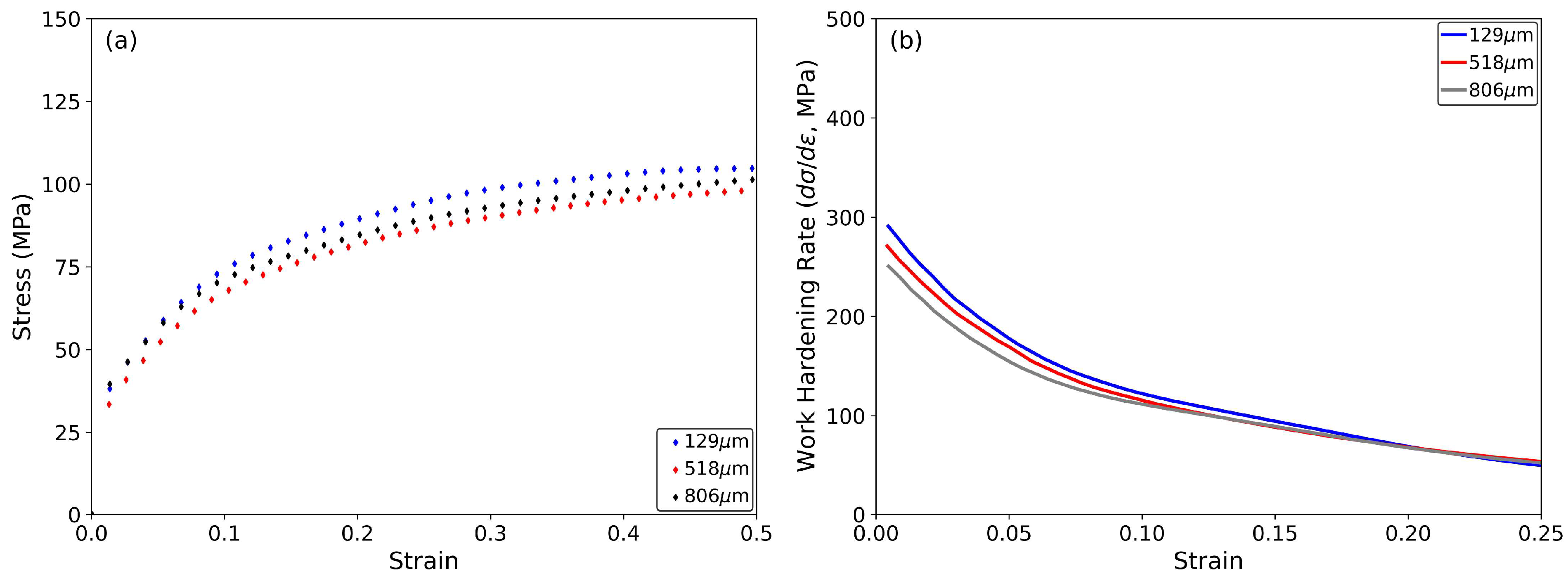
Figure 2a shows the stress–strain curves corresponding to 0.1C-Nb steel at a temperature of 1100 °C and ε ˙ = 1 s−1 as test conditions for various initial grain sizes, ranging from 129 to 806 µm. The stress–strain curves show the typical behavior observed in torsion tests. Despite minor variations in stress related to test artifacts, no clear hardening effect is evident for smaller grain sizes. Similarly, Figure 2b illustrates the instantaneous WH rate with respect to the true strain. A difference of 14.3% is measured between the WH rates corresponding to 129 and 806 µm grain sizes at the beginning of the torsion test. However, this difference reduces during the test, with WH convergence occurring for all austenite grain sizes after a strain of 0.1. Therefore, the impact of initial grain size on hardening can be considered negligible for the analyzed steels and grain size conditions. Consequently, Equation (6) has been reformulated as Equation (7):
Ω = k 1 · ε ˙ k 2 · e k 3 Q R T
In this equation, the parameters k 1 , k 2 and k 3 represent fitting constants that must be determined using the optimization method described later. Q represents the activation energy for hot deformation and will be described in more detail in the following section.

3.2. Modeling of the Dynamic Recrystallization

Several models have been proposed in the literature to establish a correlation between the mechanical behavior of DRX and the underlying metallurgical phenomena in the material in relation to the softening mechanism. Mathematical modeling of DRX is essential for understanding and predicting its behavior under different processing conditions. Various approaches have been suggested, ranging from empirical relations to physically based models. The most commonly used are the Avrami-type equations [41,42,43,44,45,46]. It is reasonable to assume that the recrystallized volume fractions are proportional to the softening observed in the flow curve [47,48,49]. In this context, DRX, being a solid-state transformation process involving nucleation and growth, can have its kinetics described by Avrami’s equation:
X D R X = 1 e β ε ε c m
where m and β are constants associated with the nucleation mechanism, and with the rate of nucleation and growth, respectively. ε c is defined as the deformation for the onset of recrystallization.
Under the hypothesis that softening is proportional to the transformed volume fractions, a similar expression to Avrami’s can be used to describe the evolution of stress during deformation, from the maximum stress to the steady state. This expression is based on the kinetics of the transformation and can be derived from an analysis of the flow curves:
σ D R X = σ s a t σ s s e · 1 e β · ε m
In this expression, σ s a t represents the saturation stress, σ s s e is the steady-state stress, and the rest of the parameters were explained earlier. The term ε c was disregarded from the previous expression (Equation (8)), as in the present study, its value is considered to be 0.

3.3. Validation of the Hyperbolic Sine Equation

While determining the complete flow curve requires a combination of the previously explained WH + DRV and DRX models (Equations (5) and (9), respectively), estimating key stress parameters within these equations, such as saturation or steady-state stress, is accomplished using the Arrhenius hyperbolic sine constitutive relation. The peak stress is widely accepted as a crucial factor in determining the constants involved in hot working. According to the Arrhenius hyperbolic sine model (see Equation (3)), the peak stress can be calculated using the following equation:
σ p e a k = 1 α s i n h 1 ε ˙ · e Q R T / A 1 n
Additionally, characteristic stresses like σ 0 , σ s a t and σ s s e can be parameterized as a function of peak stress, according to Equations (11)–(13):
σ s a t = k s a t · σ p e a k
σ 0 = k 0 · σ p e a k
σ s s e = k s s e · σ p e a k
where k s a t , k 0 and k s s e are fitting constants. These parameters are calculated using an optimization method, which will be explained in the following section. The correlation between σ s a t , σ 0 and σ s s e with σ p e a k is commonly noted in the literature, typically exhibiting a linear proportionality among them [5,24,50].
Similarly, the aim of this paper i to enhance the usefulness of the Arrhenius equation by focusing on the activation energy for hot deformation as a physically interpretable parameter. By doing so, the objective is to establish a model capable of extracting reliable and physically meaningful stresses in relation to the chemical composition. The current work adopts the approximation developed by Medina et al. for low-carbon microalloyed steels, in which the activation energy for deformation is estimated as a function of various alloying elements [51], as shown in Equation (14).
Q = 267000 2536 C + 1010 M n + 33621 S i + 35651 M o + 93681 T i 0.592 + 31637 V + 70730 N b 0.565
The remaining parameters in Equation (10), namely A , n and α , were also estimated using the work conducted by Medina et al. [51] (see Table 3).
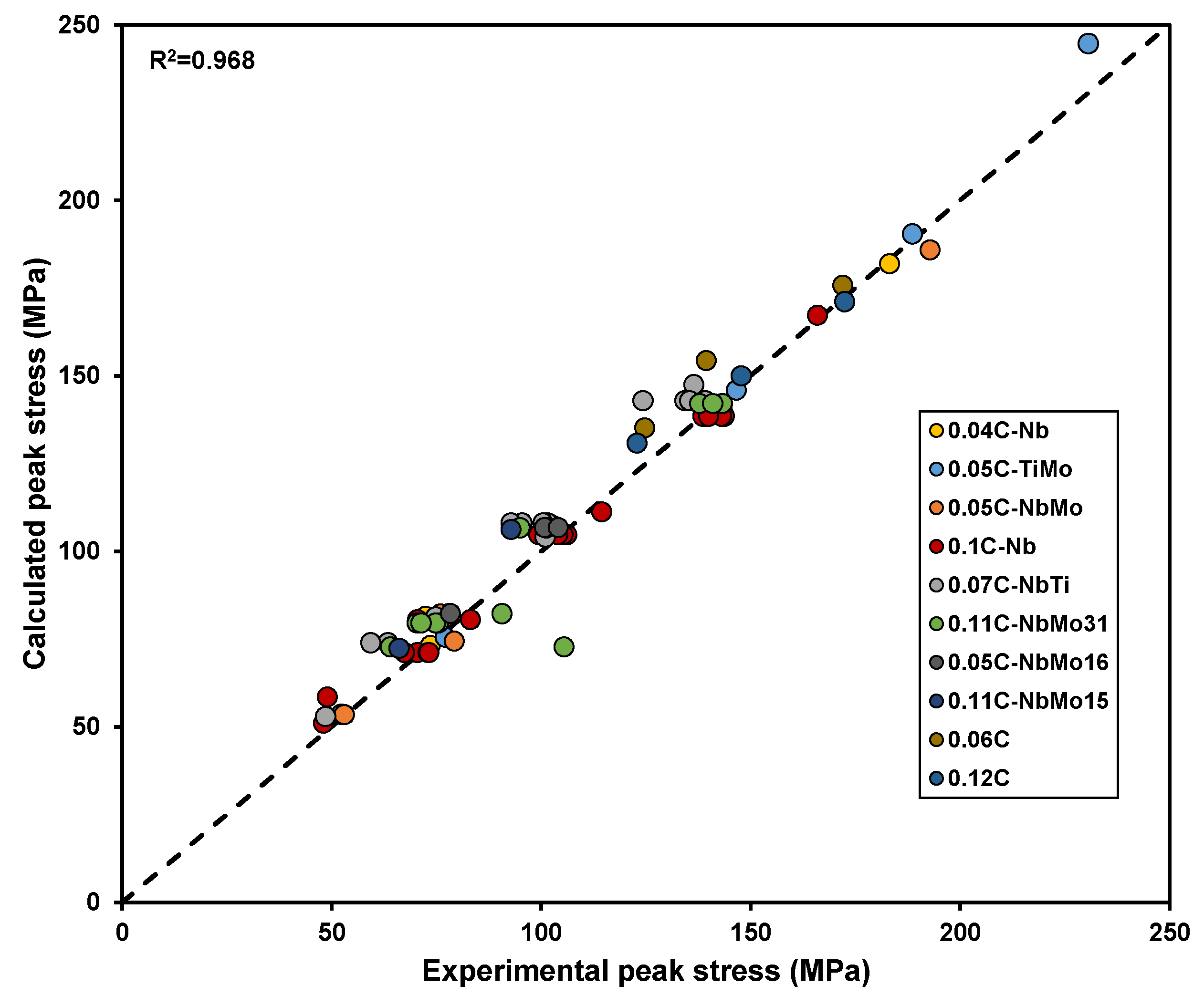
To validate the applicability of the Arrhenius equation for calculating peak stress for different compositions, a comparison was conducted between the values obtained from Equation (10) and the peak stress values derived from the experimental curves. Figure 3 shows the results of this comparison and illustrates that the estimated peak stress values are closely aligned with the experimental data. This validates the Arrhenius equation as an effective tool for estimating peak stress across a broad spectrum of chemical compositions and different temperature and strain rate conditions.

3.4. Parametrization of the Final Expression

The final equation for predicting hot working rheological behavior (see Equation (15)) combines the Arrhenius model for estimating peak stress with, on the one hand, the hardening formulation developed by Laasroui and Jonas for the WH + DRV stage [36] and, on the other hand, an Avrami-type expression for simulating softening due to DRX.
σ = σ s a t 2 + σ s a t 2 σ 0 2 · e Ω ε 0.5 σ s a t σ s s e · 1 e β · ε m
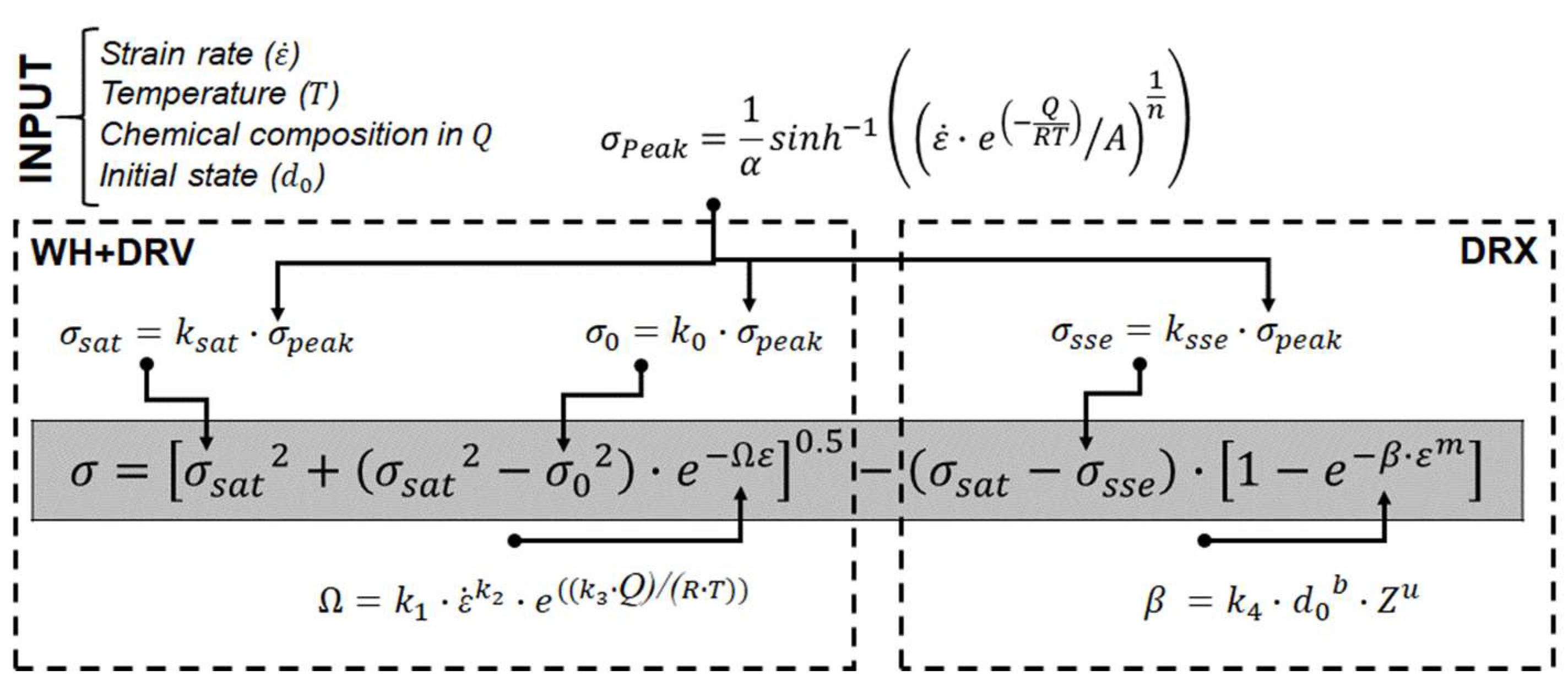
In Figure 4, the main expression (in gray, Equation (15)) and all the variables and fitting constants relevant for simulating the flow behavior are illustrated.
To fully define the expression, a total of ten fitting parameters are required: five associated with the WH + DRV stage ( k s a t ,   k 0 ,     k 1 ,   k 2 ,   k 3 ) and the remaining five related to the DRX softening stage ( k s s e ,   k 4 ,   u ,   m ,   b ).

3.5. Optimization Method

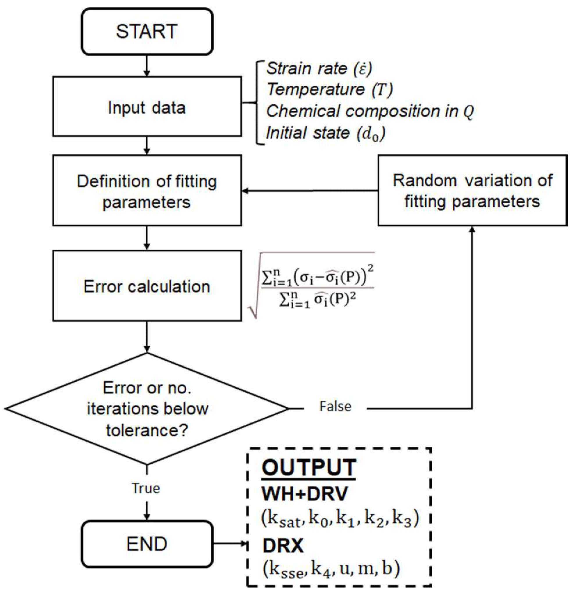
With the aim of obtaining a single mechanical hot working model robust enough to adequately simulate the behavior of different chemical compositions and different test conditions, an optimization algorithm was implemented in a Python (v 3.11.11) code. The program follows the scheme displayed in Figure 5. Firstly, it reads the experimental stress–strain curve and the chemical composition of the related steel grade. The experimental data are smoothed to reduce the model’s sensitivity to noise. Secondly, the tool compares the experimental curve with the objective function (Equation (15)). The objective function contains the phenomenological equation and the material coefficients to be fitted. It also calls for the initial set of parameters, the tolerance error, the maximum number of allowed iterations and a vector of non-negative numbers, v = v 1 ,   v 2 ,   v 3 , ,   v 10 , which dictate the random variations in the parameter updating phase. Next, an initial fitting is performed using the aforementioned initial parameters, and it is checked whether the obtained error is less than the tolerance. If so, it returns the adjusted parameters and the program stops. If not, the random variation routine is executed. This involves adding random values rn to every initial parameter with each individual value following a normal distribution with mean 0 and variance v , as defined above. The stopping criterion is defined in terms of both the error tolerance and the maximum number of iterations.
The optimization algorithm was applied to the range of test conditions listed in Table 4. The error was calculated by using the Relative Root Mean Square Error (RRMSE) formula displayed in Figure 5, with a threshold value of 0.04. The maximum number of iterations was set to 200.
This approach, which combines the stochastic variation with a least-squares-based fitting method, is designed to enhance generalizability across diverse conditions while avoiding overfitting. The model is based on a combination of physical and semi-empirical equations, each of which has a referenced physical meaning and has proven to contribute significantly to simulating observed experimental behavior. Consequently, the model’s complexity remains fixed, except for the grain size parameter, b , which was introduced to capture further aspects of the observed behavior and has proven to be particularly important. The algorithm was developed to generalize across a wide range of chemical compositions and test conditions, rather than tailoring the model to individual datasets. Consequently, while it captures overall behavioral trends in the observed data, it is unable to resolve small-scale variations. In combination with the smoothing applied to the experimental data, this approach effectively reduces the model’s sensitivity to noise, preventing overfitting. The robustness of the fitted parameters was verified by applying the model to multiple experimental conditions, as listed in Table 4.

4. Results and Discussion

4.1. Modeling of the Complete Stress–Strain Curve

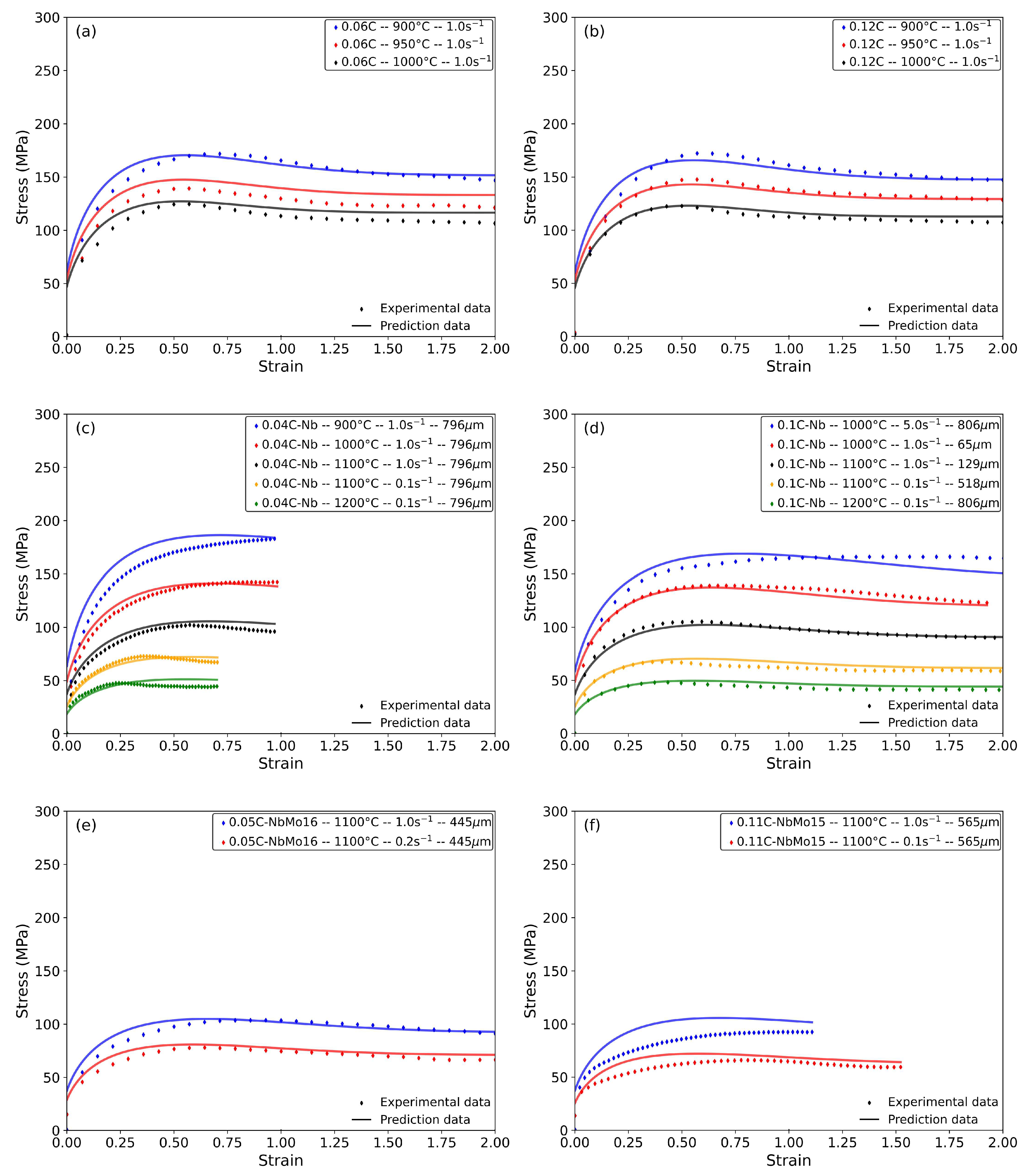
After optimizing the parameters of the constitutive equation using the previously described tool, a highly accurate expression was obtained (see Table 5), which can simulate the hot working behavior of the entire range of alloys and all the test conditions. Most of the curves corresponding to deformation temperatures above 900 °C or strain rates below 5 s−1 (low Z values) exhibit typical DRX behavior, featuring a single peak stress followed by a gradual fall towards a steady-state stress. This peak stress becomes less pronounced when the strain rate increases or the deformation temperature decreases.
Figure 6a,b show a comparison of the experimental (dotted lines) and predicted (continuous lines) flow curves for two plain carbon steels (0.06C and 0.12C) at a fixed strain rate of 1 s−1. Three different deformation temperatures of 900, 950 and 1000 °C were employed, evidencing the lowering of the flow stress as the deformation temperature decreases. The observed curves, obtained under constant strain rate conditions, demonstrate a clear correlation between stress and applied deformation temperature.
In Figure 6c,d, the stress–strain curves corresponding to two low-carbon steels (0.04 and 0.1C) microalloyed with 0.035% Nb content are depicted. The curves show the effect of various deformation temperatures and strain rates. Furthermore, the effect of initial austenite grain size (d0) on flow behavior is also evaluated for 0.1C-Nb steel. The prediction remains robust for most deformation conditions in both steels, with more pronounced errors at high Z values (deformation temperatures below 900 °C or strain rates exceeding 5 s−1), which are particularly notable in the case of 0.04C-Nb at 900 °C.
Figure 6e,f show the stress–strain curves for two chemistries with a similar Nb and Mo content (0.035 and 0.15, respectively) and two carbon levels of 0.05 and 0.11. Using a deformation temperature of 1100 °C and similar strain rates and initial grain sizes, the flow behavior of these microalloyed steels containing Nb and Mo can be robustly predicted. While the trend of reduced flow stress with carbon addition is correctly predicted, the effect of increasing carbon content (with other elements such as Nb or Mo remaining constant) is underestimated, resulting in experimental stress values that are lower than the predicted values.
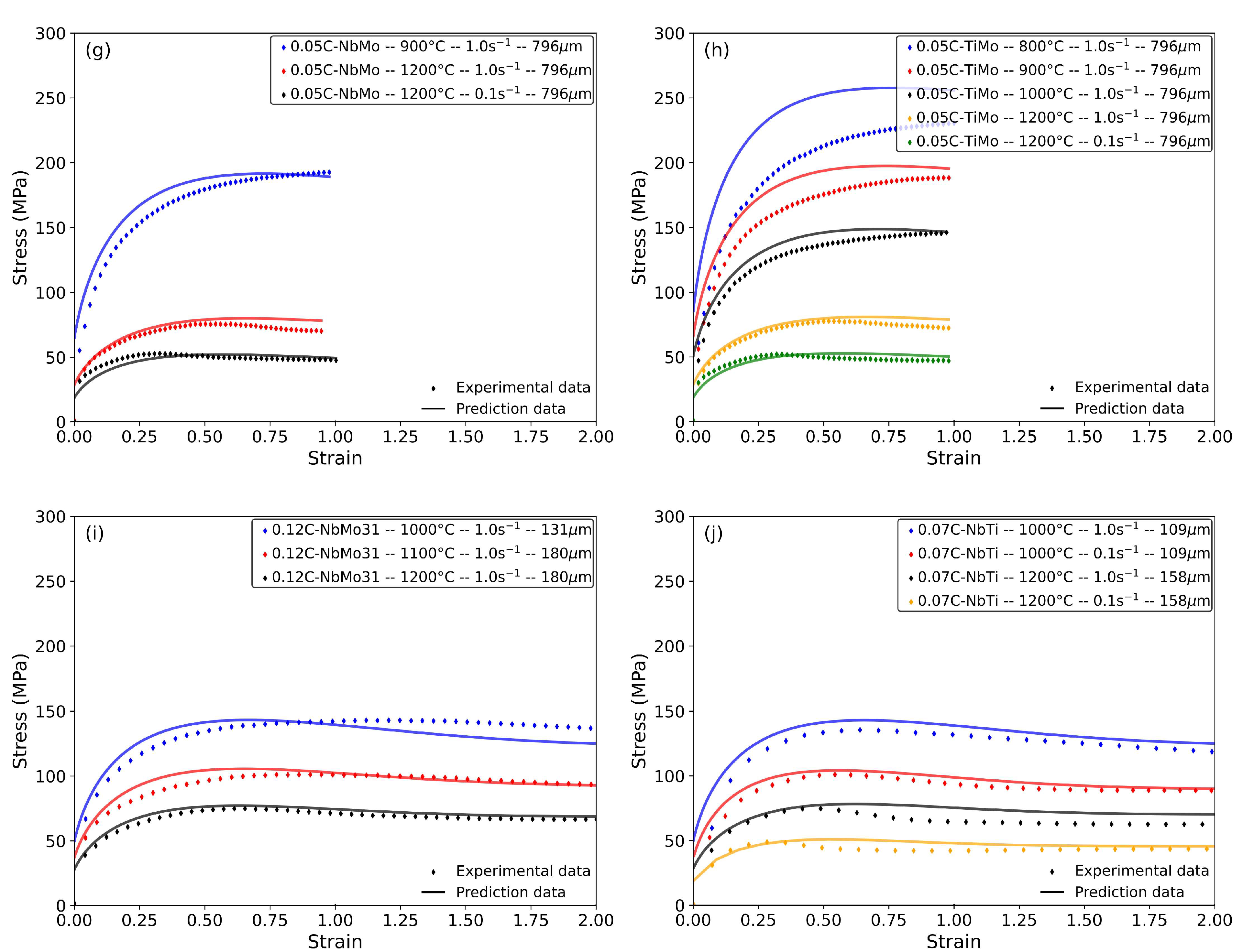
Figure 6g,h, show the stress–strain curves for 0.05C-NbMo and 0.05C-TiMo. The analysis of the two strain rates (0.1 and 1 s−1) and different deformation temperatures of 900 and 1200 °C shows that the prediction for 0.05C-NbMo steel is accurate. However, the calculated flow curves for 0.05C-TiMo chemistry deviate more significantly with a larger error, primarily associated with the analysis of lower deformation temperatures (800 °C). As previously mentioned, the current prediction is less accurate at higher Z values.
Finally, the flow curves regarding 0.12C-NbMo31 and 0.07C-NbTi chemistries are depicted in Figure 6i,j. The calculated flow curves consistently align well with the experimental data across various deformation conditions in both steels. This alignment is clearly visible in all the figures, demonstrating the effectiveness of the proposed approach for the full range of compositions.
Regarding the DRX-related parameters, the m value of 2.45 is within the range reported in the literature for low-carbon steels (1.5 to 3.5 [41,44,52,53,54,55,56,57])]. The u ( Z -related) and the b (austenite grain size-related) values, when divided by m , are equivalent to those reported for the dependence of ε p e a k and ε 0.5 in Refs. [41,44,52,53,54,55,56,57]. These parameters are within the range of 0.12–0.28 and 0.06–0.3, respectively. The current values are below these, with 0.145/2.45 ≅ 0.06 and 0.056/2.45 ≅ 0.023. The difference in the deformation mode (compression vs. torsion) may explain this discrepancy. In any case, this issue merits further analysis, which is beyond the scope of this work.
Finally, the required activation energy for DRX through the Z parameter is within the range of 288–308 kJ/mol, whereas it shows a range of 270–394 kJ/mol in the literature. Analyzing the DRV-related parameters, it is interesting to note that a similar approach to the one applied here is used for low-carbon steels in [52,55,56,57]. The reported exponents for the potential relationship of β with Z are in the range of 0.016–0.19, which is consistent with the value of 0.07 obtained in this study. The activation energy for the DRV process, on the other hand, ranges from 5 to 45 kJ/mol. The calculated energies in the present work are within 8.5–11.5 kJ/mol.

4.2. Effect of Microalloying Elements on Flow Behavior (Ti, Mo, Nb)

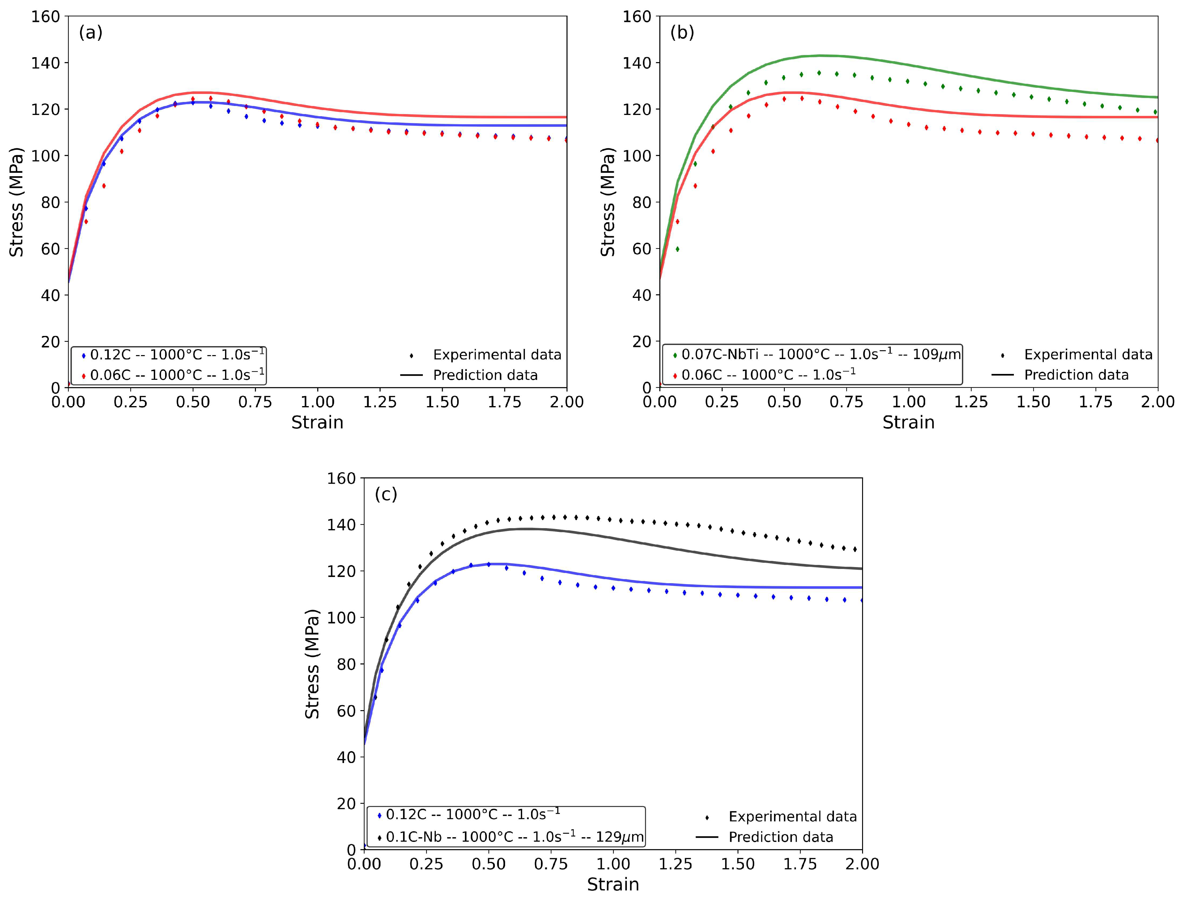
Figure 7 shows the experimental flow curves obtained at 1000 °C and a strain rate of 1 s−1 for the following chemistries: 0.06C, 0.12C, 0.07C-Ti and 0.1C-Nb. All steels were evaluated with similar initial grain sizes, ranging between 109 and 129 µm. The steel composition affects the flow curves obtained from the torsion tests. For example, the characteristic parameters related to these curves vary, e.g., the peak strain ε p , the peak stress σ p e a k etc. Regarding the impact of carbon content, slight differences are observed when comparing the flow curves corresponding to 0.06C and 0.12C (see Figure 7a). The addition of carbon promotes a slight decrement in the peak stress value, from 129 to 124 MPa, for 0.06C and 0.12C steels, respectively. The model is consistent with the trends observed in experimental curves, as higher stresses are estimated for the steel with the lowest carbon content (0.06C). This is related to the hardening effect of carbon. Higher carbon contents promote a slight softening of the steel due to increased DRV and DRX rates, thereby lowering the overall flow stress [51,52]. This trend is particularly relevant for low Z values and, in the current study, it is adequately modeled by the expression presented by Medina et al., Equation (14). The carbon-related parameter has a negative sign, leading to a decrease in the activation energy for deformation as the carbon content rises.
Figure 7b shows the flow curves for the 0.06C and 0.07C-Ti steel. A significant increase in stress is evident, which can be attributed to the addition of Ti. The effect of Ti, Mo and Nb in solid solution has been widely investigated in the literature [5,41,46]. These microalloying elements increase the activation energy for deformation and, consequently, raise the saturation stress.
Similarly, comparing the stress–strain curves of 0.12C and 0.1C-Nb steels (see Figure 7c) reveals the effect of Nb on the flow curves. As in the previous case, adding Nb increases the flow stress. The effects of the addition of Ti and Nb are accurately described by the model, in line with the hyperbolic sine equation’s predictions for peak stress values.
However, the complex interactions between alloying elements in solid solution and precipitation with DRV and DRX kinetics [41,55,56] increase the error of the prediction for such steels compared to plain carbon steels.

4.3. Effect of Austenite Grain Size

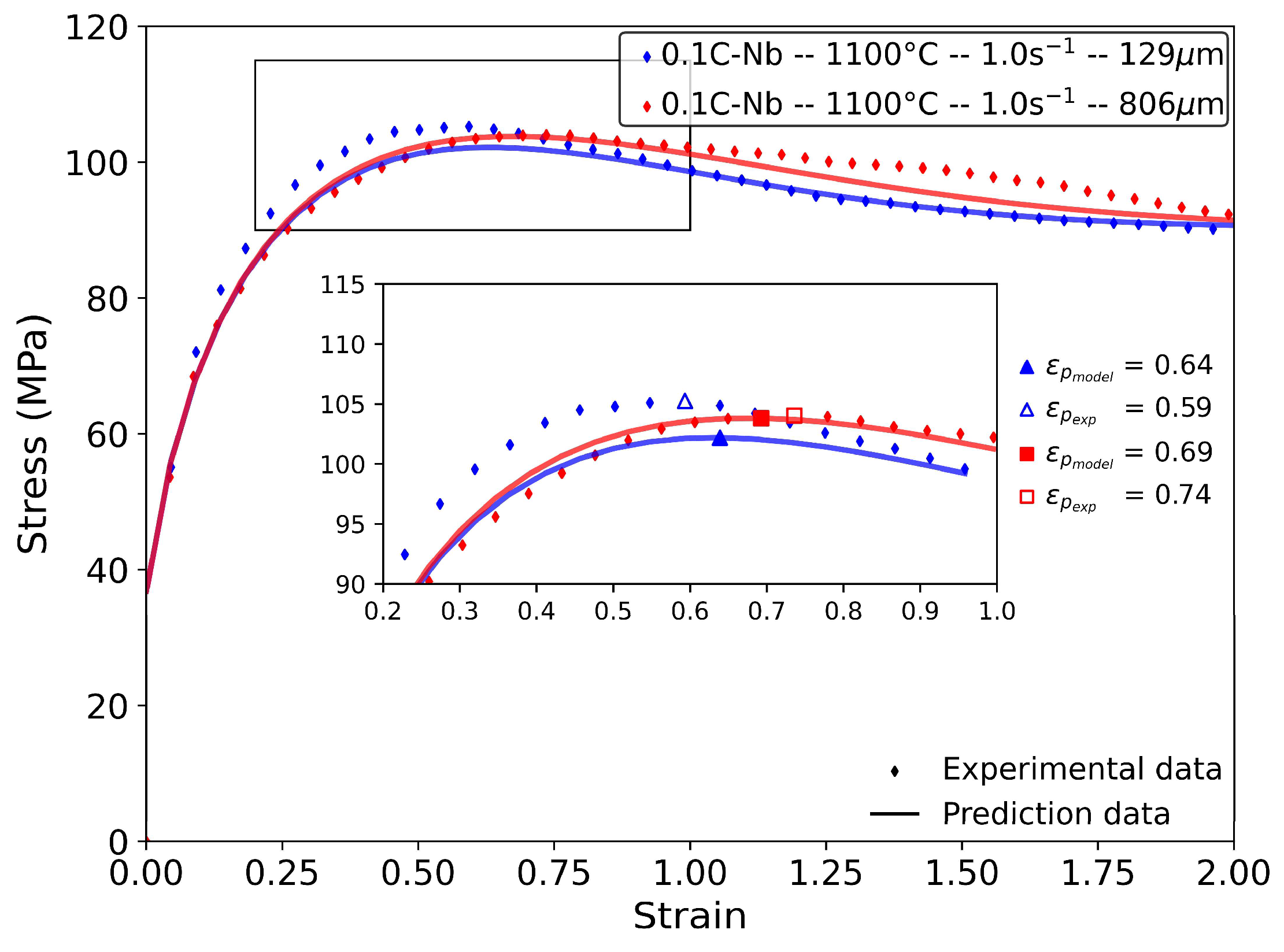
The effect of initial austenite grain size on flow curves is shown in Figure 8. The graph contains the stress–strain curves for the 0.1C-Nb material obtained at two different pre-heating temperatures of 1450 and 1150 °C, leading to different initial austenite grain sizes of 806 and 129 µm, respectively. As the reheating temperature increases, the initial grain size becomes coarser and the amount of microalloying elements in solid solution increases, leading to an increase in the peak strain value (the peak of the curve shifts to larger values). The experimental peak strain values for prior austenite grain sizes of 806 µm and 129 µm are 0.73 and 0.57, respectively., The predictions correspondingly yield values of 0.69 and 0.61 for grain sizes of 806 µm and 129 µm, respectively. Despite the error in the estimation of the peak strain, the predicted trend aligns with the experimental values. This indicates a delay in the onset of dynamic recrystallization for larger austenite grain sizes. Coarser grain sizes usually tend to produce a less pronounced fall in the stress after the peak, resulting in larger strains at the onset of the steady-state regime ( ε s s ). Examining the calculated curves reveals a correct representation of the initial grain size effect, with the peak strain value shifting towards higher values as the grain size increases.

4.4. Robustness and Limitations of the Model

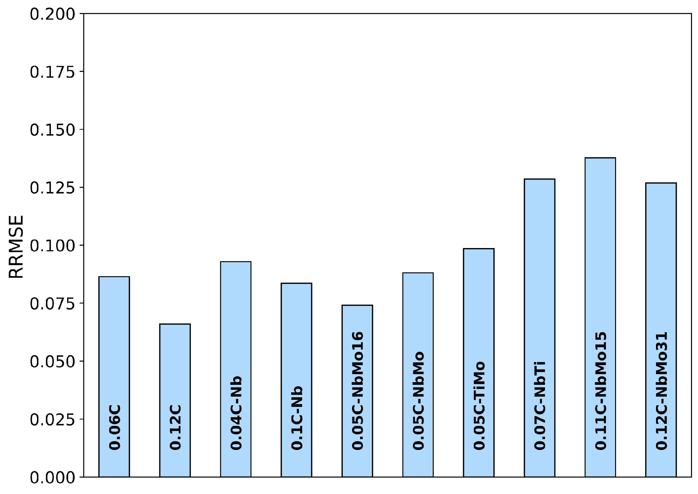
The robustness of the model is assessed in Figure 9, which shows the RRMSE values obtained for the entire range of compositions after conducting simulations at various deformation temperatures and strain rates, as listed in Table 2. The fit for all compositions is notably good, with an error of less than 14%, underscoring the suitability of the approach. This level of discrepancy is considered excellent, given the wide range covered: a temperature difference of 400 °C, strain rates ranging from 0.1 to 10 s−1, initial austenite grain sizes of up to 806 µm and ten different chemical compositions addressed by a single equation.
The model particularly excels in experimental tests at high deformation temperatures and low strain rates, showing limitations at large Z conditions, above 1013 s−1. A notable limitation is the prediction of the onset of DRX at such high Z values, which contradicts observations from experimental curves. This discrepancy is common in DRV-DRX-staged constitutive models. Such formulations typically define a critical deformation εc for DRX, and they struggle to predict pure DRV behavior regardless of the hot working conditions [5,24,55,57].
Another concern, regarding the prediction of the flow curve across wide Z values, is accuracy. This issue is commonly addressed using piecewise models [55,57]. These models divide the hot working behavior into different Z ranges, with each range being described by its own constitutive equation and set of fitting parameters. While this approach may improve prediction accuracy, it also increases the complexity of the model by introducing extra fitting parameters.
Looking at the effect of the chemical composition, Figure 9 evidences that the introduction of microalloying elements adds complexity to the flow behavior, resulting in larger errors as the chemistry becomes more alloyed. The addition of higher contents of Nb, Mo and Ti, or combinations of these microalloying elements in steel, leads to poorer predictions. Although the estimation of σ p e a k shown in Figure 3 demonstrates the robustness of the model, predicting the softening kinetics is more challenging. Interactions between different precipitate families (TiN, NbCN, etc.) and elements in solid solution with DRV and DRX kinetics require in-depth analysis.

4.5. Validation

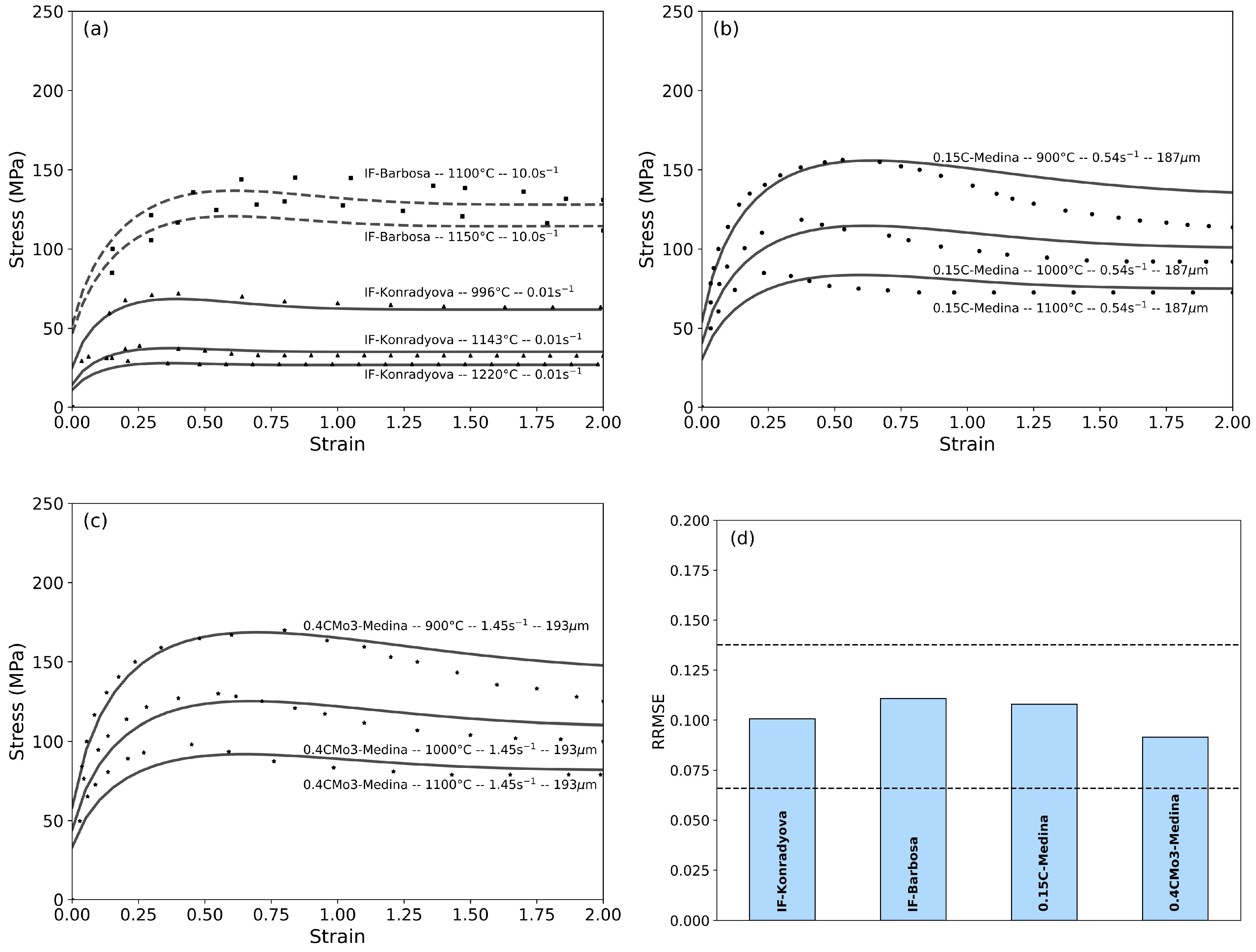
The subsequent section draws a comparison between the experimental torsion curves from the literature and the calculated flow curves. The chemical composition of the selected alloys from the literature is provided in Table 6. The effectiveness of the developed equation is assessed across a broader range of carbon content steels by examining two interstitial-free steels and two medium carbon steels (one of which is microalloyed with Mo).
Figure 10a–c show a comparison of the flow curves calculated for the aforementioned steels with those reported in the literature. The equation effectively captures the influence of chemical composition and the variations in strain rates and deformation temperatures. Figure 10d shows the RRMSE values obtained for the calculations, indicating errors that align with the tolerances observed in the low-carbon steels of the current study. Additionally, it is also worth noting that Konradyova’s data extend the Z values already used for modeling purposes (0.01 °C/s/1220 °C).

5. Conclusions

In the present study, the flow curves of ten different low-carbon steels were analyzed with the aim of developing a unified constitutive equation to reproduce the flow characteristics across a diverse range of chemical compositions and testing conditions. The following conclusions were drawn from the current investigation:
(1)
A hybrid model was devised that integrates the competition of various phenomena affecting the mechanical response of steel at high temperatures, such as strain-hardening, dynamic recovery and dynamic recrystallization. The first two mechanisms are modeled using a single dislocation-based formulation, while softening due to dynamic recrystallization is modeled using a phenomenological Avrami-type approach.
σ = σ s a t 2 + σ s a t 2 σ 0 2 · e Ω ε 0.5 σ s a t σ s s e · 1 e β · ε m
(2)
Applying the developed constitutive equation has significantly reduced the need for fitting parameters across different alloys. In particular, this formulation disregards the critical strain ε c .
(3)
The model can describe the distinct metallurgical aspects of flow behavior for different alloy compositions or testing conditions:
  • Alloys that are hot worked at higher temperatures or lower strain rates exhibit a characteristic dynamic recrystallization (DRX) behavior, characterized by a single peak stress, followed by a gradual decrease towards a steady-state stress. Conversely, the peak stress becomes less pronounced at higher strain rates or lower deformation temperatures. Clear correlations between stress and deformation temperature are observed under constant strain rate conditions, which further validates the predictive capability of the developed equation.
  • The addition of carbon slightly decreases the peak stress value due to its hardening effect. Higher carbon content promotes a slight softening of the steel due to the increased dynamic recovery (DRV) rates and DRX. The model is consistent with experimental observations and predicts higher stresses for the steel with the lowest carbon content (0.06C).
  • The influence of microalloying elements such as Ti, Mo and Nb on flow behavior is evident, with these elements contributing to an increased activation energy for deformation and higher saturation stresses. Despite the complexity introduced by the interactions between alloying elements and the precipitation kinetics, the model adequately describes the effects of these elements on the flow stress.
  • Coarser grain sizes result in a delay of DRX, thereby resulting in larger strains at the onset of the steady-state regime. The model effectively captures the impact of coarser initial austenite grain sizes on flow curves.
  • Although challenges remain in accurately predicting softening kinetics, particularly in highly alloyed steels and under high Z -value conditions ( Z > 1013 s−1), the developed equation is robust. The model exhibits low Relative Root Mean Square Error (RRMSE) values, consistently below 14%, across a broad range of compositions, initial austenite grain sizes, deformation temperatures and strain rates. Furthermore, the model has been validated using experimental torsion data from the literature, thereby expanding the range of chemical compositions to which the developed expression can be applied.

Author Contributions

Conceptualization, U.M., I.G., D.J.-B. and A.I.-M.; Methodology, U.M.; Software, S.F.-S.; Validation, U.M. and S.F.-S.; Investigation, U.M.; Writing—original draft, U.M.; Writing—review and editing, D.J.-B.; Visualization, S.F.-S.; Supervision, I.G., D.J.-B. and A.I.-M.; Project administration, I.G. and A.I.-M.; Funding acquisition, I.G. and A.I.-M. All authors have read and agreed to the published version of the manuscript.

Funding

This research was funded by the Basque Government under the following projects: Desarrollo de nuevas tecnologías y herramientas que aceleren la transición a una producción inteligente (KK-2020/00060) and Extensión de Nuevas Tecnologías y Herramientas de Digitalización para la Producción Inteligente de Componentes para Entornos Hostiles (KK-2022/00123).

Data Availability Statement

The raw/processed data required to reproduce these findings cannot be shared at this time, as the data also forms part of an ongoing study.

Conflicts of Interest

The authors declare no conflicts of interest.

References

  1. Sun, C.; Qin, Y.; Liu, Y.; Xiao, G.; Zhou, J.; Zhang, J. New constitutive model and hot processing map for A100 steel based on high-temperature flow behavior. Heliyon 2024, 10, e40823. [Google Scholar] [CrossRef] [PubMed]
  2. Lei, M.; Huang, J.; Li, Y.; Zhang, L.; Yang, G.; Wen, B. High-strain-rate mechanical constitutive modeling with computational parameters. Int. J. Plast. 2025, 189, 104329. [Google Scholar]
  3. Pasco, J.; McCarthy, T.; Parlee, J.; Nazri, N.A.; Padmajan, S.; Rodrigues, S.; Aranas, C., Jr. Constitutive modeling of modified-H13 steel. MRS Commun. 2022, 12, 343–351. [Google Scholar] [CrossRef]
  4. Solhjoo, S. Revisiting the Common Practice of Sellars and Tegart’s Hyperbolic Sine Constitutive Model. Modelling 2022, 3, 359–373. [Google Scholar] [CrossRef]
  5. Quelennec, X.; Bozzolo, N.; Jonas, J.J.; Loge, R. A new approach to modeling the flow curve of hot deformed austenite. ISIJ Int. 2011, 51, 945–950. [Google Scholar] [CrossRef]
  6. Chen, J.; Wang, J.; Jiang, H.; Wei, X.; Song, J.; Chen, Y.; Liu, S. Constitutive behavior analysis of Al-Mg-Si-Sc alloy with a two-stage physical-based model. Mater. Today Commun. 2025, 47, 113099. [Google Scholar]
  7. Donati, L.; Segatori, A.; El Mehtedi, M.; Tomesani, L. Grain evolution analysis and experimental validation in the extrusion of 6XXX alloys by use of a lagrangian FE code. Int. J. Plast. 2013, 46, 70–81. [Google Scholar] [CrossRef]
  8. Vural, M.; Caro, J. Experimental analysis and constitutive modeling for the newly developed 2139-T8 alloy. Mater. Sci. Eng. A 2009, 520, 56–65. [Google Scholar] [CrossRef]
  9. Lin, Y.C.; Chen, X.M.; Liu, G. A modified Johnson–Cook model for tensile behaviour of typical high-strength alloy steel. Mater. Sci. Eng. A 2010, 527, 6980–6986. [Google Scholar]
  10. Rusinek, A.; Klepaczko, J.R. Shear testing of a sheet steel at wide range of strain rates and a constitutive relation with strain-rate and temperature dependence of the flow stress. Int. J. Plast. 2001, 17, 87–115. [Google Scholar] [CrossRef]
  11. Zerilli, P.J.; Armstrong, R.W. Dislocation-mechanics-based constitutive relations for material dynamics calculations. J. Appl. Phys. 1987, 61, 1816–1825. [Google Scholar] [CrossRef]
  12. Voyiadjis, G.Z.; Almasri, A.H. A physically based constitutive model for fcc metals with applications to dynamic hardness. Mech. Mater. 2008, 40, 549–563. [Google Scholar] [CrossRef]
  13. Hensel, A.; Spittel, T. Kraft- und Arbeitsbedarf Bildsamer Formgeburgsverfahren; VEB Deutscher Verlag fur Grundstoffindustrie: Leipzig, Germany, 1978. [Google Scholar]
  14. Silva, M.L.N.; Pires, G.H.; Button, S.T. Damage evolution during cross wedge rolling of steel DIN 38MnSiVS5. Procedia Eng. 2011, 10, 752–757. [Google Scholar] [CrossRef]
  15. Chadha, K.; Shahriari, D.; Jahazi, M. An Approach to Develop Hansel–Spittel Constitutive Equation during Ingot Breakdown Operation of Low Alloy Steels. In Frontiers in Materials Processing, Applications, Research and Technology; Springer: Berlin/Heidelberg, Germany, 2018; pp. 239–246. [Google Scholar]
  16. El Mehtedi, M.; Musharavati, F.; Spigarelli, S. Modelling of the flow behaviour of wrought aluminium alloys at elevated temperatures by a new constitutive equation. Mater. Des. 2014, 54, 869–873. [Google Scholar] [CrossRef]
  17. Chen, X.; Si, Y.; Bai, R.; Zhang, X.; Li, Z. Hot Formability Study of Cr5 Alloy Steel by Integration of FEM and 3D Processing Maps. Materials 2022, 15, 4801. [Google Scholar] [CrossRef]
  18. Spigarelli, S.; El Mehtedi, M. A New Constitutive Model for the Plastic Flow of Metals at Elevated Temperatures. J. Mater. Eng. Perform. 2014, 23, 658–665. [Google Scholar] [CrossRef]
  19. Johnson, G.R.; Cook, W.H. A Constitutive Model and Data for Metal Subjected to Large Strains, High Strain Rates and High Temperatures. In Proceedings of the Seventh Symposium on Ballistics, The Hague, The Netherlands, 19–21 April 1983; pp. 541–547. [Google Scholar]
  20. Shokry, A.; Gowid, S.; Mulki, H.; Kharmanda, G. On the Prediction of the Flow Behavior of Metals and Alloys at a Wide Range of Temperatures and Strain Rates Using Johnson–Cook and Modified Johnson–Cook-Based Models: A Review. Materials 2023, 16, 1574. [Google Scholar] [CrossRef] [PubMed]
  21. Garofalo, F. An empirical relation defining the stress dependence of minimum creep rate in metals. Trans. Metall. Soc. AIME 1963, 227, 351–356. [Google Scholar]
  22. Sellars, C.M.; Tegart, W.J.M. Hot workability. Int. Metall. Rev. 1972, 17, 1–24. [Google Scholar] [CrossRef]
  23. McQueen, H.J.; Ryan, N.D. Constitutive analysis in hot working. Mater. Sci. Eng. A 2002, 322, 43–63. [Google Scholar] [CrossRef]
  24. Mirzadeh, H.; Cabrera, J.M.; Prado, J.M.; Najafizadeh, A. Hot deformation behavior of a medium carbon microalloyed steel. Mater. Sci. Eng. A 2011, 528, 3876–3882. [Google Scholar] [CrossRef]
  25. Rao, K.P.; Hawbolt, E.B. Development of constitutive relationships using compression testing of a medium carbon steel. J. Eng. Mater. Technol. 1992, 114, 116–123. [Google Scholar] [CrossRef]
  26. Ji, G.; Li, F.; Li, Q.; Li, H.; Li, Z. A comparative study on Arrhenius-type constitutive model and artificial neural network model to predict high-temperature deformation behaviour in Aermet100 steel. Mater. Sci. Eng. A 2011, 528, 4774–4782. [Google Scholar] [CrossRef]
  27. Nguyen-Minh, T.; Caruso, M.; Tolleneer, I.; Mayo, U.; Isasti, N.; Uranga, P.; Lorenz, U.; Duprez, L.; Akbary, F.H.; Petrov, R.; et al. Impact of Two-Phase Region Rolling on the Microstructure and Properties Distribution in Heavy Gauge Structural Steel Plate (INCROHSS)—Final Report; Publications Office of the European Union: Luxembourg, 2020; Available online: https://data.europa.eu/doi/10.2777/639791 (accessed on 18 September 2025).
  28. Pietrzyk, M.; Larzabal, G.; Uranga, P.; Isasti, N.; Jacolot, R.; Rauch, L.; Kuziak, R.; Diekmann, V.; Kitoeski, J.; Gutierrez, I.; et al. Virtual Strip Rolling Mill (VirtROLL)—Final Report; Publications Office of the European Union: Luxembourg, 2018; Available online: https://data.europa.eu/doi/10.2777/762189 (accessed on 18 September 2025).
  29. Fernandez, A. Estudio y Modelización del Conformado en Caliente de Aceros Microaleados. Aplicación a los Procesos de Laminación Directa de Formas Semiacabadas. Ph.D. Thesis, University of Navarra, Pamplona, Spain, 2001. [Google Scholar]
  30. Pereda, B. Study of the Effect of Mo Addition on the Austenite Microstructure Evolution During Hot Rolling of Nb Microalloyed steels. Application to Thin Slab Direct Rolling Technologies. Ph.D. Thesis, University of Navarra, Pamplona, Spain, 2009. [Google Scholar]
  31. Fields, D.S.; Backofen, W.A. Determination of Strain Hardening Characteristics by Torsion Testing. Proceeding Am. Soc. Test. Mater. 1957, 57, 1259–1272. [Google Scholar]
  32. Kocks, U.F. Laws for Work-Hardening and Low-Temperature Creep. ASME J. Eng. Mater. Tech. 1976, 98, 76–85. [Google Scholar] [CrossRef]
  33. Mecking, H.; Kocks, U.F. Kinetics of flow and strain-hardening. Acta Metall. 1981, 29, 1865–1875. [Google Scholar] [CrossRef]
  34. Estrin, Y.; Mecking, H. A unified phenomenological description of work hardening and creep based on one-parameter models. Acta Metall. 1984, 32, 57–70. [Google Scholar] [CrossRef]
  35. Bergstrom, Y. A dislocation model for the stress-strain behaviour of polycrystalline α-Fe with special emphasis on the variation of the densities of mobile and immobile dislocations. Mater. Sci. Eng. 1970, 5, 193–200. [Google Scholar] [CrossRef]
  36. Laasraoui, A.; Jonas, J. Prediction of steel flow stresses at high temperatures and strain rates. Metall. Trans. 1991, 22A, 1545–1558. [Google Scholar] [CrossRef]
  37. Yoshie, A.; Morikawa, H.; Onoe, Y. Formulation of Static Recrystallization of Austenite Hot Rolling Process of Steel Plate. Trans. Iron Steel Inst. Jpn. 1987, 27, 425. [Google Scholar] [CrossRef]
  38. Dunstan, D.J.; Bushby, A.J. Grain size dependence of the strength of metals: The Hall–Petch effect does not scale as the inverse square root of grain size. Int. J. Plast. 2014, 53, 56–65. [Google Scholar] [CrossRef]
  39. Wang, Y.; Huang, C.; Ma, X.; Zhao, J.; Guo, F.; Fang, X.; Zhu, Y.; Wei, Y. The optimum grain size for strength-ductility combination in metals. Int. J. Plast. 2023, 164, 103574. [Google Scholar] [CrossRef]
  40. Yasnikov, I.S.; Kaneko, Y.; Uchida, M.; Vinogradov, A. The grain size effect on strain hardening and necking instability revisited from the dislocation density evolution approach. Mater. Sci. Eng. A 2022, 831, 142330. [Google Scholar] [CrossRef]
  41. Fernandez, A.I.; Uranga, P.; Lopez, B.; Rodriguez-Ibabe, J.M. Dynamic recrystallization behavior covering a wide austenite grain size range in Nb and Nb-Ti microalloyed steels. Mater. Sci. Eng. A 2003, 361, 367–376. [Google Scholar] [CrossRef]
  42. Shaban, M.; Eghbali, B. Determination of critical conditions for dynamic recrystallization of a microalloyed steel. Mater. Sci. Eng. A 2010, 527, 4320–4325. [Google Scholar] [CrossRef]
  43. Liu, C.; Barella, S.; Peng, Y.; Guo, S.; Liang, S.; Sun, J.; Gruttadauria, A.; Belfi, M.; Mapelli, C. Modeling and characterization of dynamic recrystallization under variable deformation states. Int. J. Mech. Sci. 2023, 238, 107838. [Google Scholar] [CrossRef]
  44. Jonas, J.J.; Quelennec, X.; Jiang, L.; Martin, E. The Avrami kinetics of dynamic recrystallization. Acta Mater. 2009, 57, 2748–2756. [Google Scholar] [CrossRef]
  45. Li, X.; Duan, L.; Li, J.; Wu, X. Experimental study and numerical simulation of dynamic recrystallization behavior of a microalloyed plastic mold steel. Mater. Des. 2015, 66, 309–320. [Google Scholar] [CrossRef]
  46. Mirzadeh, H.; Najafizadeh, A. Prediction of the critical conditions for initiation of dynamic recrystallization. Mater. Des. 2010, 31, 1174–1179. [Google Scholar] [CrossRef]
  47. Avrami, M. Kinetics of phase change: I General theory. J. Chem. Phys. 1939, 7, 1103–1112. [Google Scholar] [CrossRef]
  48. Avrami, M. Kinetics of phase change: II Transformation–time relations for random distribution of nuclei. J. Chem. Phys. 1940, 8, 212–224. [Google Scholar] [CrossRef]
  49. Avrami, M. Granulation, phase change, and microstructure kinetics of phase change. J. Chem. Phys. 1941, 9, 177–184. [Google Scholar] [CrossRef]
  50. de Sousa Sulzbach, G.A.; Goncalves Rodrigues, M.V.; Rodrigues, S.F.; Macedo, G.M.E.; de Abreu, H.F.G.; Aranas, C., Jr.; Silva Reis, G.; Santos Silva, E. Constitutive analysis of stress–strain curves in dynamic softening of high Nb- and N-containing austenitic stainless-steel biomaterial. J. Mater. Res. Technol. 2022, 19, 4939–4956. [Google Scholar] [CrossRef]
  51. Medina, S.F.; Hernandez, C.A. General expression of the Zener Hollomon parameter as a function of the chemical composition of low alloy and microalloyed steels. Acta Mater. 1996, 44, 137–148. [Google Scholar] [CrossRef]
  52. Serajzadeh, S.; Taheri, A.K. An investigation into the effect of carbon on the kinetics of dynamic restoration and flow behavior of carbon steels. Mech. Mater. 2003, 35, 653–660. [Google Scholar] [CrossRef]
  53. Marques Ivaniski, T.; de Souza, T.F.; Épp, J.; da Silva Rocha, A. Constitutive Modelling of High Temperature Flow Behaviour for a Low Carbon High Silicon Bainitic Steel. Mater. Res. 2020, 23, e20200264. [Google Scholar] [CrossRef]
  54. Cao, R.; Wang, W.; Ma, S.; Yan, H.; Mu, Z.; Zhang, S. Arrhenius constitutive model and dynamic recrystallization behavior of 18CrNiMo7-6 steel. J. Mater. Res. Technol. 2023, 24, 6334–6347. [Google Scholar] [CrossRef]
  55. Peng, Y.; Guo, S.; Liu, C.; Barella, S.; Liang, S.; Gruttadauria, A.; Mapelli, C. Dynamic recrystallization behavior of low-carbon steel during hot rolling process: Modeling and simulation. J. Mater. Res. Technol. 2022, 20, 1266–1290. [Google Scholar] [CrossRef]
  56. Wang, L.; Ji, L.; Yang, K.; Gao, X.; Chen, H.; Chi, Q. The Flow Stress–Strain and Dynamic Recrystallization Kinetics Behavior of High-Grade Pipeline Steels. Materials 2022, 15, 7356. [Google Scholar] [CrossRef] [PubMed]
  57. Xu, Y.; Birnbaum, P.; Pilz, S.; Zhuang, X.; Zhao, Z.; Kräusel. Investigation of constitutive relationship and dynamic recrystallization behavior of 22MnB5 during hot deformation. Results Phys. 2019, 14, 102426. [Google Scholar] [CrossRef]
  58. Konrádyová, J.; Longauerová, M.; Jonšta, P.; Jonšta, Z.; Longauer, S.; Girman, V.; Vojtko, M.; Borûta, A.; Matvija, M.; Fujda, M.; et al. Hot ductility of TiNb IF steel slab after hot torsion testing. Metals 2019, 9, 752. [Google Scholar] [CrossRef]
  59. Viella, J.J.; Barbosa, R. Prediction of Stress–Strain Curves of Hot Deformed If Austenite. ISIJ Inter. 2002, 42, 319–321. [Google Scholar] [CrossRef]
  60. Hernandez, C.A.; Medina, S.F.; Ruiz, J. Modelling austenite flow curves in low alloy and microalloyed steels. Acta Mater. 1996, 44, 155–163. [Google Scholar] [CrossRef]
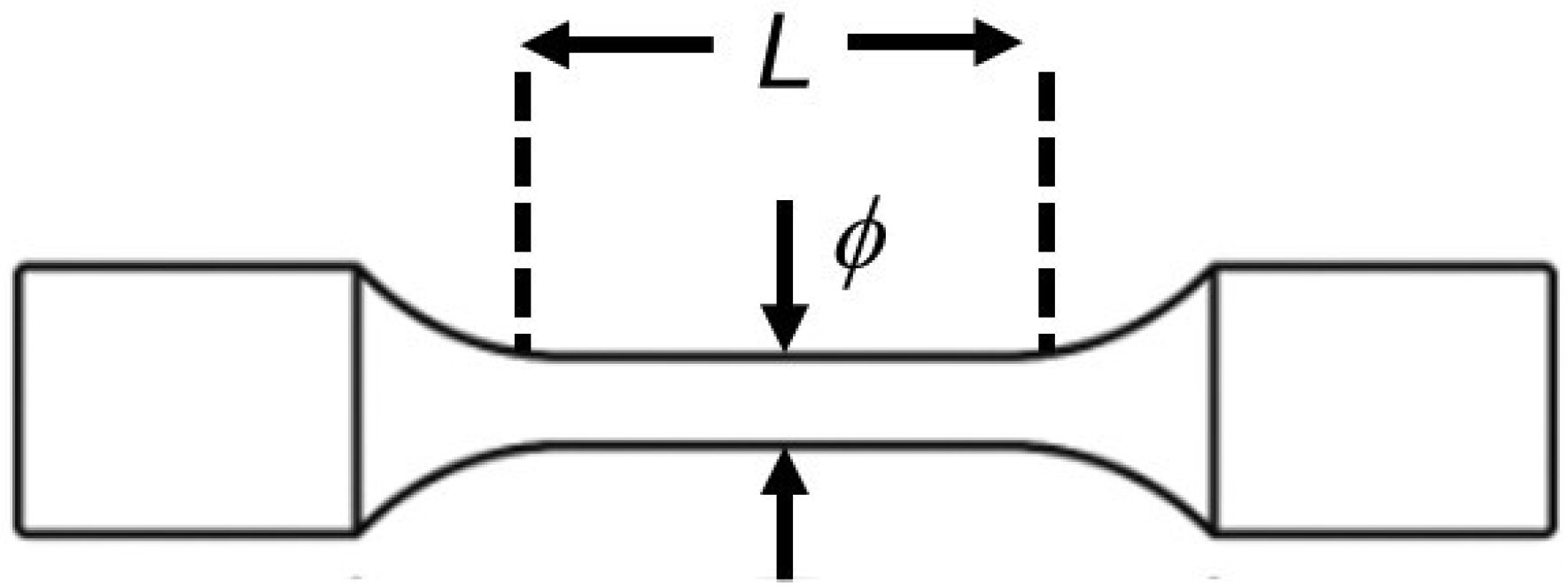
Figure 1. Drawing of the torsion test specimen.
Metals 15 01044 g001
Figure 2. (a) Stress–strain curves up to ε = 0.5 and (b) instantaneous WH rate corresponding to different initial grain sizes of 129, 518 and 806 µm for a deformation temperature of 1100 °C and a strain rate of 1 s−1.
Metals 15 01044 g002
Figure 3. Calculated vs. experimental peak stress values.
Metals 15 01044 g003
Figure 4. Scheme of the full model for hot working.
Metals 15 01044 g004
Figure 5. Flowchart of the implemented method. The program follows a loop that aims to reduce the resulting error of predicted stress.
Metals 15 01044 g005
Figure 6. Experimental (scatter points) vs. predicted (continuous lines) flow curves for the entire selection of chemistries. (a) 0.06C, (b) 0.12C, (c) 0.04C-Nb, (d) 0.1C-Nb, (e) 0.05C-NbMo16, (f) 0.11C-NbMo15, (g) 0.05C-NbMo, (h) 0.05C-TiMo, (i) 0.12C-NbMo31 and (j) 0.07C-NbTi.
Metals 15 01044 g006aMetals 15 01044 g006b
Figure 7. Comparison between experimental vs. predicted stress–strain curves obtained at 1000 °C deformation temperature and strain rate 1 s−1 for (a) 0.06C vs. 0.12C, (b) 0.12C vs. 0.07C-Ti and (c) 0.12C vs. 0.1C-Nb steel.
Metals 15 01044 g007
Figure 8. Impact of initial grain size on experimental and calculated flow curves for 0.1C-Nb steel.
Metals 15 01044 g008
Figure 9. Estimated RRMSE value for each chemistry tested at different strain rates and deformation temperature conditions listed in Table 2.
Metals 15 01044 g009
Figure 10. (ac) Comparison between the experimental and calculated flow curves for the steels from Table 6. The solid line represents the predicted stress–strain curve, while the dashed lines correspond to experimental data. (d) Calculated Relative Root Mean Square (RRMSE) values for the steels presented in the literature, with dotted lines indicating the error boundaries obtained for the steels under study.
Metals 15 01044 g010
Table 1. Chemical composition of the selected steels (wt%).
Steel ReferenceCMnSiMoTiNbRef
0.06C0.061.540.250.0050.0020.002[27]
0.12C0.121.520.250.0050.0020.001[27]
0.04C-Nb0.041.550.20.0030.0020.034[28]
0.1C-Nb0.11.420.310.0050.0020.035[29]
0.05C-NbMo160.051.580.040.160.0020.03[30]
0.11C-NbMo150.111.430.330.150.0070.033[30]
0.05C-TiMo0.051.610.20.20.090.003[28]
0.05C-NbMo0.051.60.210.210.0040.035[28]
0.07C-NbTi0.070.620.010.0050.0670.034[29]
0.12C-NbMo310.121.460.310.310.0040.034[30]
Table 2. Test conditions for the different chemistries.
Steel ReferenceInitial Austenite Grain Size (µm)Strain Rate (s−1)Temperature (°C)
0.04C-Nb-0.11100
1200
1900
1000
1100
1200
0.05C-TiMo-0.11100
1200
1800
900
1000
1200
0.05C-NbMo-0.11100
1200
1900
1200
0.1C-Nb220.11100
0.21100
11000
1100
650.11100
11000
12911000
1100
5180.11100
11000
1100
8060.11100
1200
0.21000
1100
1200
11000
1100
51000
0.07C-NbTi6011000
1090.11000
1100
11000
1100
101100
1580.11100
1200
11000
1100
1200
39211000
1100
79611000
1100
0.12C-NbMo311310.11100
11000
1100
1200
18011000
1100
1200
5500.11100
6500.21100
11200
66011000
1200
0.05C-NbMo1636511100
4450.21100
11100
0.11C-NbMo155650.11100
11100
0.06C-1900
950
1000
0.12C-1900
950
1000
Table 3. Parameters for Equation (13).
Parameter
A ( 12.197 + 65.59 C 49.052 N b ) · e x p ( 0.00007076 Q )
n 4.458
α 0.011875
Table 4. Range of hot working conditions used for modeling the mechanical behavior of steel grades shown in Table 1.
Test ConditionStrainStrain Rate (s−1)Temperature (°C)
Minimum0.750.1800
Maximum2101200
Table 5. Estimated values for the fitting parameters obtained by the optimization method.
Fitting Parameters k s a t k 0 k 1 k 2 k 3
DRV1.090.351.7−0.070.03
Fitting parameters k s s e k 4 u m b
DRX0.8680−0.1452.45−0.056
Table 6. Chemical composition and hot working conditions of the steels selected for the validation process (wt%).
Steel ReferenceCMnSiMoTiNbRef
IF-Konradyova0.0030.330.0070.0020.0330.038[58]
IF-Barbosa0.00280.150.010.0010.0830.002[59]
0.15C-Medina0.150.740.21---[60]
0.4CMo3-Medina0.420.790270.18--[60]
Disclaimer/Publisher’s Note: The statements, opinions and data contained in all publications are solely those of the individual author(s) and contributor(s) and not of MDPI and/or the editor(s). MDPI and/or the editor(s) disclaim responsibility for any injury to people or property resulting from any ideas, methods, instructions or products referred to in the content.