Constitutive Modeling of Creep–Fatigue Interaction in 1Cr-1Mo-0.25V Steel for Hold-Time Testing

Abstract

In the field of energy production, creep–fatigue interaction is a typical failure mode that might compromise the structural integrity of both rotating equipment and pressure vessels. Common design practices approach the problem in a conservative way by using high safety factors, which typically results in additional costs for manufacturing companies. The aim of this article, in the framework of continuum damage mechanics approaches, is to present a novel fatigue damage-based constitutive law. The presented law is directly inspired by well-assessed creep-based rules, suggesting a similarity in the behavior. On the other hand, creep deformation and damage are calculated with a more recent approach. The identification of the model parameters was carried out by interpreting experimental results obtained from low-cycle fatigue and creep relaxation tests performed on a commonly used ferritic–martensitic steel for power generation rotor forgings. To validate the proposed models, they were used to estimate material life consumption when the material was subjected to fully reversed axial loading conditions with hold time under tensile load. Different loading conditions at different total strain ranges and hold times were simulated, and good agreement was found between the predicted and experimental life, thus confirming the validity of the proposed models.

1. Introduction

The future energy market outlook predicts a consistent increase in renewable energy sources, which are expected to overtake traditional energy sources with the goal of reducing CO₂ emissions.

At the same time, the increase in renewable energy production has deeply affected the mix of power production in many countries. Industrial segments such as combined cycle plants (CCPs) have been especially affected by these modifications. With time, these assets have progressively switched from base-load to peak-load production, balancing the intermittent production of wind and solar plants. Consequently, CCPs have been forced to improve their fast start-up capability, making their design more and more challenging for turbomachinery manufacturers.

This scenario comes together with the global demand for an increase in the maximum allowed inlet temperature and pressure for both steam and gas turbines, considering the efficiency boost associated with a higher maximum temperature of the thermodynamic cycle. This temperature increase usually does not come together with the relaxation of the strict flexible operability constraints, such as start-up times, maintenance intervals, and number of cycles at end of life. An application where these trends are particularly stressed is also the implementation of expanders in concentrated solar plants (CSPs).

In this direction, in recent years, several works that aimed to increase the flexible operability of steam and gas turbines operating in CSPs and CCPs have been published [1]. Another research trend looks at implementing smarter control loops that manage start-up requirements, such as the maximum allowed stress or strain during turbine start-up [2,3].

The underlying structural phenomena that have to be taken into account during the design of turbomachinery operating at high temperature under variable loading are creep and low-cycle-fatigue (LCF) induced by thermal loads. While, in the past, these two phenomena and their interaction could be addressed through rather conservative design rules and simple calculations, the market trends described up to now require much more advanced tools capable of capturing many aspects of the life consumption process.

At elevated temperatures, the combination of mechanical and thermal cyclic stresses can initiate and propagate cracks faster than predicted by the sequential analysis of creep and LCF life consumption [4,5]. The interaction of creep and fatigue results in complex failure modes [6], including enhanced crack initiation due to cyclic plastic strain and accelerated crack growth facilitated by creep mechanisms such as grain boundary sliding and void nucleation. Studies have been conducted on the effect of prior creep on fatigue and of prior fatigue on creep, showing that both damage mechanisms exert a reciprocal influence on each other owing to their softening effect on the material [7].

Looking at turbomachinery components, rotors represent a bottleneck for reductions in start-up time, usually being exposed to the highest temperature in the flow path of rotating equipment while having a higher heat capacity, usually resulting in the worst combination of creep and thermal fatigue damage. In addition, the rotor design usually needs to exclude the nucleation of cracks on their surface, since vibrations might lead to fast crack growth from thermally induced flaws. The application of fracture mechanics approaches, as a consequence, has limited applications in the area of the external surface of the rotor. However, the fracture mechanics methodology can be useful in developing damage-tolerant approaches to assess the criticality of forging defects below the rotor surface.

Common conservative design rules for pressurized components are also extended to the design of turbomachinery components such as casing and rotors. Examples are given by the guidelines outlined in the ASME Boiler and Pressure Vessel Code [8] and the R5 assessment procedure for the high-temperature response of structures [9].

The ASME Boiler and Pressure Vessel Code (BPVC), more specifically section III (for nuclear components) and section VIII (for pressure vessels), provides a framework for evaluating high-temperature design through design-by-analysis (DBA) methods. For creep–fatigue, the ASME BPVC incorporates a creep–fatigue damage summation. This approach typically uses a linear or bilinear damage rule, combining cyclic fatigue damage (based on the strain range and fatigue life) with creep damage (based on rupture life fractions) to assess total damage per cycle.

The ASME BPVC is considered conservative and ensures a high safety margin, often simplifying complex interactions to enable practical design evaluations. Just to help grasp the conservative approach followed by ASME, we can observe that after assessing the separate damage due to creep and fatigue, the BPVC prescribes the use of bilinear diagrams to assess the allowable combined damage fraction. Just to give an example, for materials such as the 9Cr-Mo-V class, ASME allows for only a 1% creep damage fraction for a 10% fatigue damage fraction, creating a challenging scenario for designers working in this field.

In contrast, the R5 procedure developed in the United Kingdom for high-temperature plant assessments provides a more mechanistic and comprehensive treatment of creep–fatigue interaction. This methodology incorporates the detailed modeling of cyclic plasticity and creep strain evolution under service conditions, thereby enabling explicit predictions of strain accumulation and stress relaxation.

With respect to creep–fatigue interaction, R5 employs combined interaction diagrams that account for the synergistic effects of creep and fatigue more accurately than linear summation approaches. Compared with the ASME BPVC methodology, the R5 framework is generally less conservative, as it seeks to provide realistic life predictions by explicitly considering the actual material response in service. This feature makes R5 particularly relevant for high-temperature plant life extension and defect tolerance assessments.

Nevertheless, both methodologies inevitably rely on simplifying assumptions to facilitate their application within the context of industrial design. To achieve a more fundamental understanding of the governing degradation mechanisms, alternative approaches should be considered, including those based on continuum damage mechanics (CDM).

In particular, constitutive models based on CDM have enabled the development of “unified” approaches [10,11,12] for creep–fatigue damage assessment, enabling the simultaneous evaluation of different degradation mechanisms within a single theoretical framework. For instance, in the Lemaitre formulation [10,11], the damage rate is expressed as directly proportional to the plastic strain rate once a critical threshold of accumulated inelastic strain has been exceeded.

It should be emphasized that although this approach permits the simultaneous evaluation of fatigue and creep damage within a unified computational framework, significant challenges may arise in calibrating the interaction between the two mechanisms, particularly with respect to the evolution of creep curves (see [12]). In such situations, it becomes necessary to develop separate yet interacting models for low-cycle fatigue (LCF) and creep, followed by the adoption of an appropriate summation rule. To circumvent these limitations, the approach proposed in this study deliberately departs from Lemaitre-type models, instead formulating an innovative relationship for the assessment of LCF damage (see Section 3.1.1). The analysis presented herein is applied to a representative steel grade commonly employed in turbine rotor forgings, with specific attention to operating conditions where frequent turbine start-ups exacerbate the effects of steady-state service within the creep regime.

Future developments will extend the proposed methodology to additional classes of steels, such as 9Cr-1Mo-V and 12Cr-1Mo-V alloys, which are extensively employed in power generation applications and for which a substantial body of creep–fatigue investigations is available in the literature (e.g., [13,14,15,16,17]). Moreover, the predictive capabilities of the model will be evaluated under complex loading scenarios, including service-like thermomechanical fatigue (TMF) conditions [18,19].

Within this context, the present study introduces an original approach for the combined assessment of creep–fatigue damage and illustrates its applicability to a representative heat-resistant ferritic–martensitic steel typically employed in rotor forgings. Beyond the development of constitutive models for cyclic plasticity and creep damage, particular emphasis is placed on the definition of innovative relationships for damage evaluation and on a consistent parameter identification strategy. The outcomes are validated against experimental data, thereby highlighting both the predictive accuracy of the approach and its potential relevance for life assessment of components operating under demanding service conditions.

2. Materials and Methods

2.1. Materials

2.1.1. Chemical Composition and RT Properties

The investigated material corresponded to the ASTM A470 class 8 alloy, classified as a 1Cr-1Mo-0.25V heat-resistant steel. This alloy is commonly used for forgings of steam turbine rotors and gas turbine disks operating in the temperature range of 500 °C to 560 °C. It is a low-alloy, medium-carbon steel with good creep resistance within this temperature interval [20]. The material was supplied in the conventional quenched and tempered condition. The evaluated chemical composition, consistent with the ASTM A470 class 8 specification, is reported in the first row of

Table 1. Chemical composition requirements (wt%) of ASTM A470-8 steel (first row) and chemical composition of the steel tested in [21,22] (second row).

C	Si	Mn	P	S	Ni	Cr	Mo	V	Fe
0.25–0.35	0.15–0.35	≤1.00	≤0.015	≤0.018	≤0.75	0.90–1.50	1.00–1.50	0.20–0.30	BAL.
0.29	0.30	0.74	0.006	0.003	0.39	1.12	1.16	0.25	BAL.

.

For the subsequent evaluation of the creep damage model parameters (Section 2.2.2), the creep-rupture data reported in the NIMS database [21,22] are employed, since this kind of test entails a considerable amount of time. The chemical composition of the steel tested by NIMS is shown in the second row of Table 1. It is possible to see that the latter falls within the ASTM A470 class 8 standard range.

The heat treatment under which the investigated material has undergone is also similar to that described in the NIMS report, and the similarity between these two steels is corroborated by the comparison between the tensile properties and the hardness measured after heat treatments on the forged piece (

Table 2. Tensile properties at RT of ASTM A470- class 8 steel tested in [21,22].

	Rm (MPa)	Rp 0.2 (MPa)	${\mathit{\epsilon }}_{\%}$ (%)	Z (%)	HB
Tests	790 ± 4.21	648 ± 3.45	15 ± 2.217	55.5 ± 4.51	249 ± 3.27
NIMS	790–830	620–690	17–19	57–63	235–252

).

To determine the tensile properties at room temperature (RT), six specimens were extracted from the forging. The mean values and standard deviations of the measured tensile properties are reported in the first row of Table 2.

In Table 2 (second row), the minimum and maximum values of hardness and tensile properties are also reported for the nine different steels examined in [21,22]. The heat treatment applied to the investigated material was similar to that described in the NIMS study, and the similarity between the two steels is further supported by the comparison of tensile properties and hardness measured after the respective heat treatments of the forged specimens (Table 2).

The consistency between the NIMS data and the investigated material is particularly valuable, as it supports the assumption of using the creep data to inform the selected constitutive models and enables their validation in terms of the number of cycles to rupture using LCF tests with hold time (Section 3.2). Conversely, the conducted LCF and LCF with hold-time (HT) testing campaign (Section 2.1.3) provides the basis for identifying the parameters of isotropic and kinematic hardening (Section 2.2.1), LCF damage (Section 3.1.1), and secondary creep models (Section 2.2.2). It should be noted that within the presented framework, the NIMS LCF tests with hold time are not included in the parameter identification process; consequently, they serve exclusively as the validation component of the constitutive models.

2.1.2. High-Temperature Mechanical Behavior

From the comparison of the characteristics and properties of the investigated material with those of the alloy studied in [21,22] (see Table 1 and Table 2), it can be concluded that no significant differences exist between the material under investigation and ASTM A470 class 8. Therefore, it is reasonable to expect that the alloy examined exhibits creep behavior within the temperature range of 500–560 °C similar to that of ASTM A470 class 8, for which the creep data are summarized in

Table 3. Sample mean and standard deviation for creep-rupture data at 500 °C of ASTM A470 class 8 steel tested in [21,22].

$\mathit{\sigma }$ (MPa)	${\mathit{m}}_{{\mathit{t}}_{\mathit{R}}}$ (h)	${\mathit{s}}_{{\mathit{t}}_{\mathit{R}}}$ (h)	${\mathit{m}}_{{\mathit{\epsilon }}_{\mathit{R}}}$ (%)	${\mathit{s}}_{{\mathit{\epsilon }}_{\mathit{R}}}$ (%)
373	464	384	20.55	4.53
333	2564	1228	20.75	4.10
314	3100	250	22.50	4.95
294	14718	6214	18.11	4.04
265	53490	21440	14.22	4.87
235	127116	30590	12.00	2.45

.

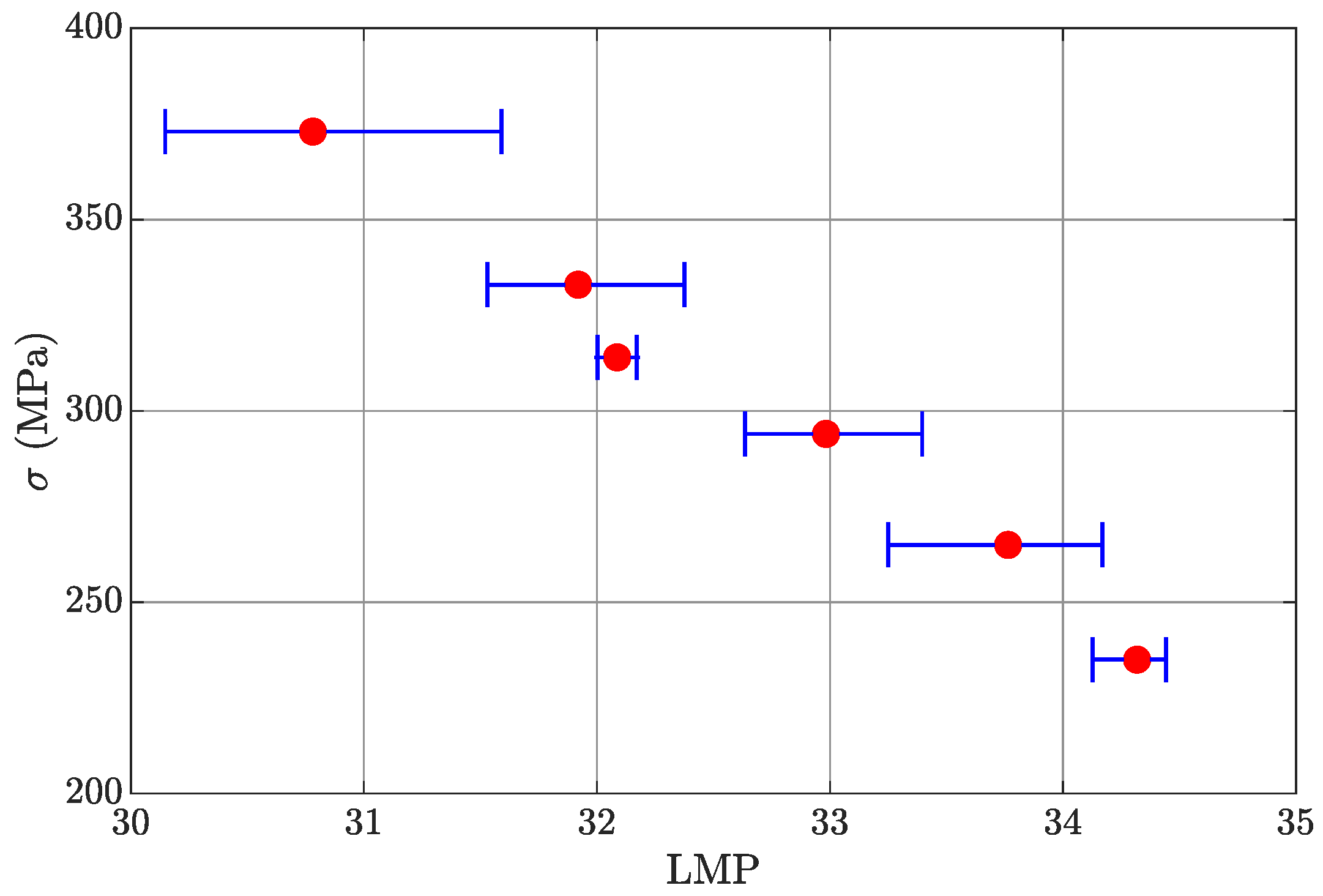
In order to show the dispersion of stress-rupture data the Larson–Miller parameter (LMP) is calculated using Equation (1):

$$\mathrm{LMP}={\displaystyle \frac{T}{1000}}·\left(C+{log}_{10}{t}_R\right)$$

(1)

The value of C was determined through regression [23,24,25]. Specifically, C corresponds to the value that minimizes the quadratic error in the fit of the $\sigma$–LMP points using a second-degree polynomial. The obtained value of C was 19.57, which is consistent with values reported in [23] for medium-Cr martensitic steels at the same temperature. The results are illustrated in Figure 1, where the mean values and associated error bars of the data are displayed.

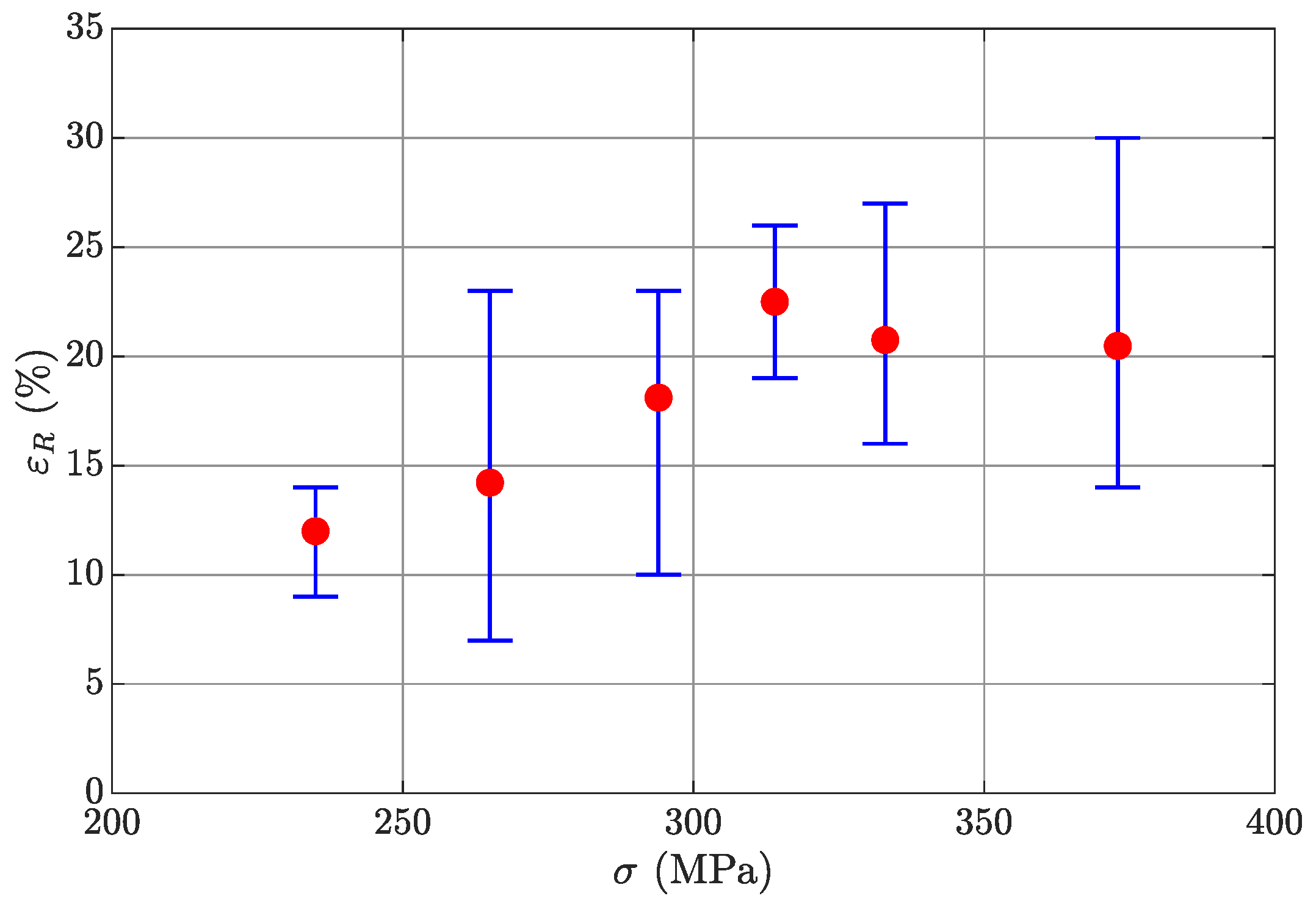
For the same reason, the dispersion of creep-rupture strain at 500 °C is presented in Figure 2. It can be observed that the initial upward trend of the mean values levels off at higher stress levels. The highlighted error bands fall within the typical range for creep data.

2.1.3. Testing Campaign

An experimental campaign was conducted to characterize fatigue damage in the LCF regime at 500 °C. Total strain ranges of $0.40$, $0.60$, $0.65$, $0.80$, $0.90$, $1.00$, and $1.20\%$ were selected to investigate damage phenomena under conditions representative of the actual service environment of steam turbine rotors.

The tests were performed in accordance with ASTM E606/E606M-12 using a servohydraulic testing machine (Schenck, Darmsatdt, Germany) with a maximum load capacity of 100 kN, equipped with an induction oven. Test control was carried out using a high-temperature axial extensometer with a gauge length of $25.4$ mm (1 inch).

To evaluate the interaction between creep and fatigue damage mechanisms, two additional LCF tests with a total strain range of $\mathsf{\Delta }\epsilon =0.60\%$ and a hold time of $t_H=30$ s were conducted. The testing campaign is summarized in

Table 4. Identification codes (ID) assigned to the 12 tests conducted and experimental parameters.

ID	$\mathbf{\Delta }\mathit{\epsilon }(\%)$	${\mathit{t}}_{\mathit{H}}$ (s)	T (°C)	Load Ratio	$\dot{\mathit{\epsilon }}\left({\mathit{s}}^{-1}\right)$	Wave Function
A	0.60	30	500	−1	$3·{10}^{-3}$	Triangular
B	0.60	30	500	−1	$3·{10}^{-3}$	Triangular
C1	1.20	0	500	−1	$3·{10}^{-3}$	Triangular
C2	1.00	0	500	−1	$5·{10}^{-3}$	Triangular
C3	0.90	0	500	−1	$3·{10}^{-3}$	Triangular
C4	0.80	0	500	−1	$5·{10}^{-3}$	Triangular
C5	0.80	0	500	−1	$5·{10}^{-3}$	Triangular
C6	0.65	0	500	−1	$3·{10}^{-3}$	Triangular
C7	0.60	0	500	−1	$6·{10}^{-3}$	Triangular
C8	0.60	0	500	−1	$6·{10}^{-3}$	Triangular
C9	0.40	0	500	−1	$6·{10}^{-3}$	Triangular
C10	0.40	0	500	−1	$3·{10}^{-3}$	Triangular

, where each test is identified by an individual ID. The expected number of cycles to failure for the tests ranged from ${10}^2$ to ${10}^4$ cycles. The selected strain ranges are representative of the typical operational strain levels of the components under service conditions.

The selection of a triangular waveform was motivated by its closer representation of the loads experienced by the components of interest during thermal transients. To validate the constitutive models presented in this study, a comparison between the simulations and the NIMS LCF data with hold time at the same temperature (available in [21,22]) is presented in Section 3.2.

2.2. Methods

In this section, the constitutive models and the methods employed for the evaluation of their parameters are presented. First, the cyclic plasticity model, the creep model, and the creep damage model are introduced. The parameters of the two damage models are determined independently based on creep and LCF tests, and the total damage is calculated as their linear summation [11,12,26,27,28]. The detailed procedure for calculating and combining the damage contributions is described in Section 2.2.4.

2.2.1. Cyclic Plasticity Model

For the description of cyclic plasticity behavior, a nonlinear hardening model is considered the most appropriate, while the basic von Mises criterion is employed for the yield surface, without the need to invoke more complex frameworks. In this section, the essential details are outlined for clarity, whereas a more comprehensive discussion can be found in the existing literature [10,11]. The model combines the nonlinear isotropic hardening formulation by Voce with the exponential kinematic hardening model by Chaboche. Under these assumptions, the yield surface is expressed as in Equation (2).

$$f=\sqrt{{\displaystyle \frac{3}{2}}({\sigma }_{ij}^D-{\chi }_{ij}^D):({\sigma }_{ij}^D-{\chi }_{ij}^D)}-{\chi }_{tot}-R-{\sigma }_Y.$$

(2)

It is useful to note that for the simple case of a tension–compression test, Equation (2) reduces to a scalar equation:

$$f=\sigma -{\chi }_{tot}-R-{\sigma }_Y.$$

(3)

The total back-stress, ${\chi }_{tot}$, is assumed, in accordance with a well-known approach proposed by Chaboche, to be the superposition of multiple back-stresses [10,11]. total backstress, ${\chi }_{tot}$, is assumed, following the well-established approach proposed by Chaboche, to be the superposition of multiple backstresses [10,11].

In the present study, three backstresses are employed for the accurate modeling of the selected steam turbine rotor steel. This choice is supported by the comparison with hysteresis cycles obtained from experimental tests and is also recommended by Chaboche for practical applications [11]. As shown in Section 3.1.3, this number of backstresses is sufficient to reproduce the stress–strain response within a reasonable margin of error.

Each component of the backstress tensor is assumed to evolve proportionally to the combined contributions of the plastic strain rate, ${\dot{\epsilon }}_{pl}$, and creep strain rate, ${\dot{\epsilon }}_{cr}$. Within the framework of continuum damage mechanics, we assume an isotropic damage variable as follows:

$${\dot{\chi }}_{ij}^{\left(k\right)}=\left[C_{ij}^{\left(k\right)}\left({\dot{\epsilon }}_{pl}+{\dot{\epsilon }}_{cr}\right)-{\gamma }_{ij}^{\left(k\right)}{\chi }_{ij}^{\left(k\right)}(\dot{p}+{\dot{p}}_{cr})\right]·(1-D).$$

(4)

On the other hand, the isotropic component of hardening evolves as a function of the accumulated plastic and creep strain, according to the relationship by Voce. Again, in the framework of continuum damage mechanics, still under the assumption of an isotropic damage variable, this leads to the following:

$$R=Q\left[1-e^{-b(p+p_{cr})(1-D)}\right].$$

(5)

The evaluation of Chaboche kinematic hardening and Voce isotropic hardening is based on the methodology presented in [29], which requires only two hysteresis cycles and the corresponding peak stress values at a given temperature. The main advantage of this method lies in its reduced computational effort. Additionally, the proposed approach allows for the inclusion of up to four backstresses, enhancing the accuracy of the model, particularly in the plastic-knee region of the stress–strain curve.

Alternative methods for the identification of Chaboche constants rely on more sophisticated algorithms, such as genetic approaches [30,31].

For the present case study, the procedure was applied to two cycles corresponding to total strain ranges of $\mathsf{\Delta }\epsilon =0.90$.

2.2.2. Creep Strain and Damage Modeling

The comparison presented in Section 2.1.1 supports the use of NIMS creep data for the creep damage model applied to the investigated material.

The selection of an appropriate creep model within the framework of a creep–fatigue assessment for turbine rotor steel requires careful consideration of multiple factors. The creep model must be coupled with a suitable damage model, compatible with the LCF model and appropriate for the specific alloy under investigation.

For the selected alloy, the basic creep model developed by Dorn [26], which relates the secondary creep strain rate to the applied stress, is considered satisfactory. The model can be expressed mathematically as

$${\dot{\epsilon }}_{cr}=A·e^{B\sigma }$$

(6)

For the present testing campaign, the creep model was calibrated using the relaxation part of the high-temperature LCF tests with hold time. Specifically, the creep parameters were determined from the third hysteresis cycle of each temperature set. In contrast, the parameters used to describe the time to rupture, $t_R\left(\sigma \right)$, and the creep-rupture strain, ${\epsilon }_R\left(\sigma \right)$, were obtained from the stress-controlled tests reported in the NIMS experimental campaign [21,22].

During the hold time, the following expression is employed to describe the evolution of stress relaxation:

$$\sigma \left(t\right)=-{\displaystyle \frac{1}{B}}ln\left[AE(t-t_0)B+e^{-B{\sigma }_0}\right]$$

(7)

With regard to creep damage, numerous models are available [32]; for instance, the Kachanov model [33] is a well-established approach. However, for the present material, it has been observed that adopting a more advanced formulation than the classical Kachanov model may provide improved predictive capability.

Consequently, considering the good agreement of the Dorn model with experimental data, the sine-hyperbolic creep damage (SINH) model [34] has been selected. This model represents a modification of the creep damage formulation proposed in [35]. The conventional SINH damage model is expressed by the following system of equations (Equation (8)), in which the McVetty secondary creep strain rate is employed [26]:

$$\left\{\begin{array}{c}{\dot{D}}_{cr}={\displaystyle \frac{Q_c\left(1-e^{-\phi }\right)}{\phi }}sinh{\left({\displaystyle \frac{\sigma }{{\sigma }_T}}\right)}^{{\chi }_c}{e}^{\phi D_{cr}}\hfill \\ {\dot{\epsilon }}_{cr}=K·sinh\left({\displaystyle \frac{\sigma }{{\sigma }_s}}\right)·e^{\lambda D_{cr}^r}\hfill \end{array}\right.$$

(8)

with all the parameters depending on temperature and stress and being always positive. Unlike the Kachanov model, in the ${\dot{\epsilon }}_{cr}$ term, there is not the conventional effective stress but the exponential term $e^{\lambda D_{cr}^r}$, which is responsible for the nonlinear evolution of ${\epsilon }_{cr}$ (integrating with constant $\sigma$).

It might seem that in this model, the damage rate is dependent on the stress, but actually, its derivation lies in the need to obtain an expression that utilizes the strain rate expression. In other words, if the equations are properly rearranged, the stress disappears, and the damage rate can be expressed as a function of strain and strain rate.

This model is often tuned on the basis of stress-imposed creep tests [26,34,35,36]. For the present testing campaign, data fitting has shown that a slightly modified expression—where $\phi$ is allowed to be negative—can further improve the quality of data fitting, especially when creep relaxation tests are used to feed the model. The integration of the expression for the damage rate, under the assumption of a constant stress value, leads to Equation (9):

$$D_{cr}\left(t\right)=-{\displaystyle \frac{1}{\left|\phi \right|}}ln\left[1-{\displaystyle \frac{\left|\phi \right|}{\phi }}\left(1-e^{-\phi }\right)Q_{c}sinh{\left({\displaystyle \frac{\sigma }{{\sigma }_T}}\right)}^{{\chi }_c}t\right].$$

(9)

From the last expression, the rupture time $t_R$ can be identified by imposing $D_{cr}=1$ (under the assumption that the rupture occurs when the damage is equal to the unity):

$$t_R\left(\sigma \right)={\displaystyle \frac{1}{Q_c·sinh{\left({\displaystyle \frac{\sigma }{{\sigma }_T}}\right)}^{{\chi }_c}}}.$$

(10)

In the present approach, it was observed that to improve the fit with experimental data, the dependence of the strain rate on stress should be modeled as exponential rather than proportional to the hyperbolic sine. Consequently, the constitutive expression for the strain rate is

$${\dot{\epsilon }}_{cr}=A{e}^{B\sigma }·e^{\lambda D_{cr}^r}.$$

(11)

By imposing $r=1$ and integrating the previous system of differential equations for a constant value of $\sigma$, a creep strain law can be obtained as a function of time:

$${\epsilon }_{cr}\left(t\right)={\displaystyle \frac{A{e}^{B\sigma }·t_R}{\left(1-{\displaystyle \frac{\lambda }{\left|\phi \right|}}\right){\displaystyle \frac{\left|\phi \right|}{\phi }}\left(1-e^{-\phi }\right)}}\left\{1-{\left[1-{\displaystyle \frac{\left|\phi \right|}{\phi }}\left(1-e^{-\phi }\right){\displaystyle \frac{t}{t_R}}\right]}^{1-{\displaystyle \frac{\lambda }{\left|\phi \right|}}}\right\}.$$

(12)

An analytical closed-form expression for the evolution of strain as a function of time is of particular interest. This is because, although the three parameters $Q_c$, ${\chi }_c$, and ${\sigma }_T$ appear in the $t_R\left(\sigma \right)$ function (Equation (10)), once they are determined solely from experimental rupture time data, $\lambda$ and $\phi$ remain as the only parameters to be identified. By setting $t=t_R$ in Equation (12) and substituting the dependence of $t_R$ on $\sigma$, an expression for ${\epsilon }_R\left(\sigma \right)$ can be derived.

Finally, the function employed for the estimation of the parameters $\lambda$ and $\phi$ is defined as the ratio between the rupture time, $t_R$, and the creep-rupture strain, ${\epsilon }_R$, which depends on a simplified function of the stress, $\sigma$:

$${\displaystyle \frac{t_R\left(\sigma \right)}{{\epsilon }_R\left(\sigma \right)}}={\displaystyle \frac{\left(1-{\displaystyle \frac{\lambda }{\left|\phi \right|}}\right){\displaystyle \frac{\left|\phi \right|}{\phi }}\left(1-e^{-\phi }\right)}{A{e}^{B\sigma }\left\{1-{\left[1-{\displaystyle \frac{\left|\phi \right|}{\phi }}\left(1-e^{-\phi }\right)\right]}^{1-{\displaystyle \frac{\lambda }{\left|\phi \right|}}}\right\}}}.$$

(13)

2.2.3. Lcf Damage Modeling

The fundamental concept underlying the proposed LCF damage model formulation is to derive the fatigue damage accumulation rule from a well-established creep damage approach within the continuum damage mechanics framework, such as the Kachanov–Rabotnov model [33].

$$\left\{\begin{array}{c}{\dot{\epsilon }}_{cr,KR}=A_{KR}·{\tilde{\sigma }}^m=A_{KR}·{\left({\displaystyle \frac{\sigma }{1-D_{KR}}}\right)}^m\hfill \\ {\displaystyle \frac{\mathrm{d}{D}_{KR}}{\mathrm{d}t}}=B_{KR}·{\displaystyle \frac{{\sigma }^k}{{(1-D_{KR})}^f}}\hfill \end{array}\right..$$

(14)

The underlying concept employed here is the introduction of an effective stress into the Norton creep strain rate equation, coupled with a creep damage rate that depends on a given power of stress. This formulation clearly exhibits a strong resemblance to Norton’s secondary creep model. As is well known, the resulting creep model is capable of predicting the transition from the secondary to the tertiary creep phase. Considering that LCF damage, when plotted against accumulated plastic strain, exhibits a trend similar to that described by Kachanov for creep [10,11], the proposed model for the accumulation of LCF damage is expressed as follows (Equation (15)):

$${\displaystyle \frac{d{D}_p}{dp}}={\displaystyle \frac{M_p{\left(\dot{p}\right)}^{{\chi }_p}}{{(1-D_p)}^{{\varphi }_p}}}$$

(15)

The model is derived by considering the second equation of the Kachanov model and substituting stress with the accumulated plastic strain rate. Furthermore, the damage derivative is evaluated with respect to p rather than time, since LCF damage is associated with time-independent plasticity and therefore cannot be time-dependent. By removing the direct dependence on stress, which varies during LCF cycling, significant advantages are achieved in terms of parameter identification.

The concept of employing a creep damage model framework for LCF damage is also discussed in [37], where the authors utilized the creep damage formulation by Murakami and Liu [35]. Nonetheless, as explained in the previous section, for the present modeling campaign, the Kachanov approach serves solely as a reference to derive the LCF damage rule and is not applied to compute actual creep damage.

The model can also be reformulated as follows (Equation (16)), explicitly highlighting its dependence on the strain rate:

$${\displaystyle \frac{d{D}_p}{dt}}={\displaystyle \frac{M_p{\left(\dot{p}\right)}^{{\chi }_p+1}}{{(1-D_p)}^{{\varphi }_p}}}.$$

(16)

This expression highlights, indeed, the limit of this kind of approach: high strain rate cycling determines a higher damage rate. This might not appear desirable for every possible application of the model. In any case, proper adjustment of the parameters makes the model suitable for low strain rates, observed in the thermal loading of turbomachinery. When considering this specific loading case, LCF damage is mostly driven by the accumulation of plastic strain, while the increase in the damage rate due to the plastic strain rate can be neglected due to very slow loading conditions.

By integrating Equation (15) with p, the evolution is shown in (17):

$$D_p\left(t\right)=1-{\left[1-M_p{\left(\dot{p}\right)}^{{\chi }_p}({\varphi }_p+1)p\right]}^{{\displaystyle \frac{1}{{\varphi }_p+1}}}=1-{\left(1-{\displaystyle \frac{p\left(t\right)}{p_R}}\right)}^{{\displaystyle \frac{1}{{\varphi }_p+1}}}.$$

(17)

From the previous equation, the form of the accumulated rupture plastic strain can be inferred, in direct analogy with the time to rupture in the Kachanov–Rabotnov creep damage model:

$$p_R={\displaystyle \frac{1}{M_p{\left(\dot{p}\right)}^{{\chi }_p}({\varphi }_p+1)}}.$$

(18)

This quantity depends solely on the plastic strain rate, $\dot{p}$, which can be conveniently estimated as a mean value for a specific loading condition.

In the present experimental data set, not all stress and strain information over the entire test duration is available. In such cases, the total plastic strain at rupture can be estimated using Equation (19):

$$p_R=2·N_R\mathsf{\Delta }{\epsilon }_{p,mid}$$

(19)

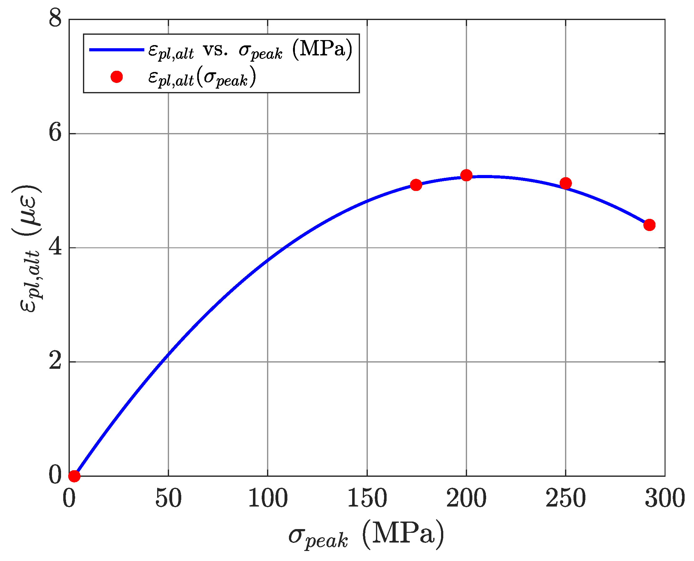
For tests with multiple cycles, the alternating plastic strain and the peak tensile stress can be recorded and fitted, imposing that at ${\sigma }_{peak}=0$ (i.e., rupture), the alternating plastic strain, ${\epsilon }_{pl,alt}$, is zero.

Equation (17) indicates that the plastic damage reaches unity when $p=p_R$, and the nonlinearity of the damage curve is controlled by the parameter ${\varphi }_p$. From Equation (18), it is evident that the two parameters, $M_p$ and ${\varphi }_p$, are redundant. One approach to resolve this redundancy is to evaluate damage for a given cycle by calculating the reduction in elastic modulus induced by void formation [10,11], assuming that for this steel, LCF damage causes a measurable change in stiffness:

$$D_{exp}=1-{\displaystyle \frac{\tilde{E}}{E}}$$

(20)

Therefore, it is now possible to use Equation (21) by solving for ${\varphi }_p$ and obtaining the necessary parameter in (18).

$${\varphi }_p={\displaystyle \frac{log\left(1-\frac{p}{p_R}\right)}{log\left(1-D_{exp}\left(p\right)\right)}}-1.$$

(21)

Once the value of ${\varphi }_p$ has been determined, it is feasible to fit $p_R$ versus $\dot{p}$ with a power-law relationship according to Equation (18).

2.2.4. Schematic Summary of the Proposed Constitutive Models

The model proposed here distances itself from other viscoplastic approaches, such as those described in [10,11,12,26,38,39], due to the separation of the inelastic strain in a plastic strain fraction and in a creep strain fraction. Hence, the model can be summarized by the following set:

• The total strain is

  $$\epsilon ={\epsilon }_{el}+{\epsilon }_{pl}+{\epsilon }_{cr}.$$

  (22)
• The evolution of LCF damage is given by Equation (15).
• The evolution of creep damage is given by Equation (8).
• The total damage $D_{tot}$ is the linear sum [11,26,27] of the two damages:

  $${\dot{D}}_{tot}={\dot{D}}_{cr}+{\dot{D}}_p.$$

  (23)
• The yield function for the simple case of tension–compression monoaxial loading is given by Equation (2).
• The evolution of the generic backstress for kinematic hardening is given by Equation (4) (where the damage in input is $D_{tot}$).
• The evolution of the isotropic hardening variable is given by Equation (5) (where the damage in input is $D_{tot}$ and the accumulated strain is the sum of creep and plastic strain).

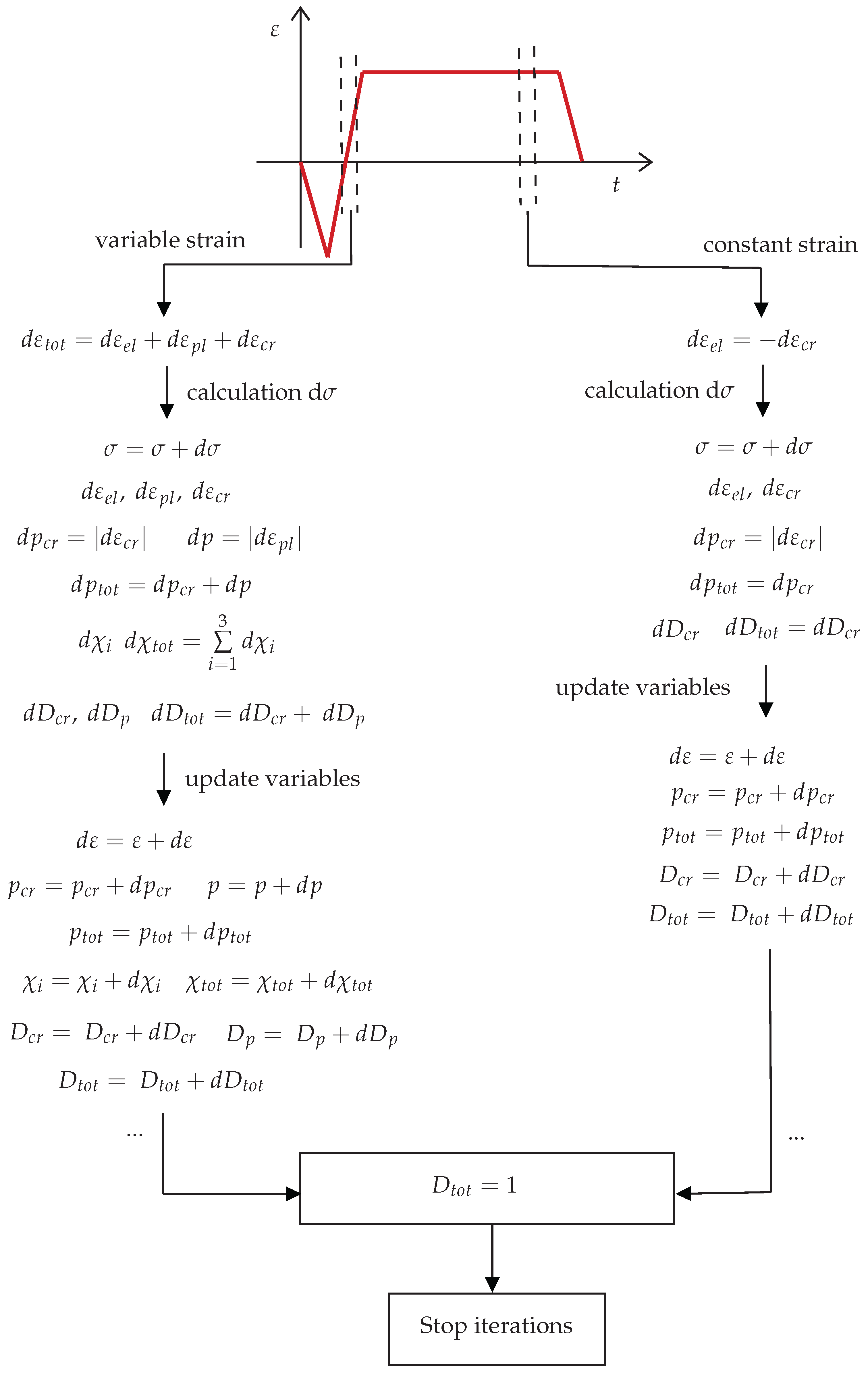
It is noteworthy that each damage evolution depends on the total accumulated damage, rather than solely on its current value. This feature allows the model to account for the interaction between creep and fatigue. The implementation of the model is summarized in the algorithm presented in Figure A1.

Initially, the strain history is divided into a sequence of smaller increments. From the total strain increment, the corresponding stress increment is computed. The stress, along with the various strain components—accumulated plastic strain, creep strain, backstress components, and damage components—is then updated for the next increment. This process is iterated until failure occurs, defined by $D_{tot}=1$.

3. Results and Discussion

In this section, the results of the parameter fitting procedure, the evaluated model parameters, and the outcomes of the numerical implementation of the constitutive models for the 1Cr-1Mo-0.25V material (see Section 2.1.1) are presented. For the latter, the loading condition of $\mathsf{\Delta }\epsilon =0.60\%$ with $t_H=30$ s is reproduced, and a comparison between the third cycle and the midlife cycle of the experimental tests is analyzed. Additionally, in Section 3.2, other loading conditions are considered, and the simulated life is compared with the experimental data reported in [21,22].

All fitting procedures were performed using the ordinary least squares (OLS) method.

3.1. Model Identification and Parameter Estimation

3.1.1. Plasticity and LCF Damage

The parameters of the Chaboche–Voce nonlinear kinematic hardening model (Equations (4) and (5)), obtained following the procedure described in [29] using the hysteresis cycles at $\mathsf{\Delta }\epsilon =0.90\%$ and $\mathsf{\Delta }\epsilon =0.65\%$, are reported in Table 6. It should be noted that the term ${\sigma }_Y$ listed in Table 6 does not correspond to the conventional yield strength (i.e., Rp₀₂), but rather to the stress at which linearity is lost and the exponential terms begin, according to the method presented in [29].

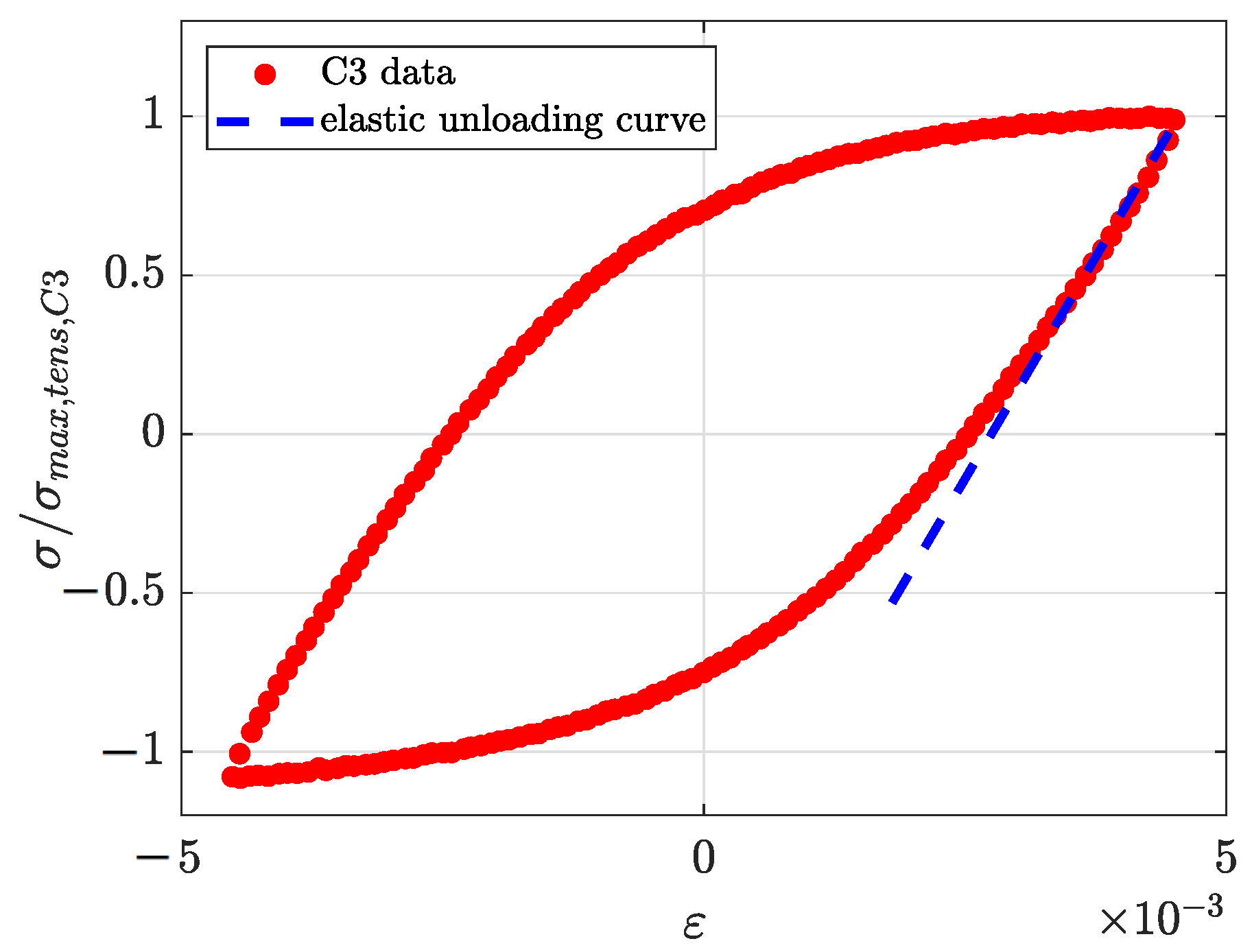
The Young’s modulus was determined by fitting the elastic unloading part of the stress–strain curve from the peak tensile stress of the third hysteresis cycle of test C3 (Figure 3). The third cycle was selected to minimize experimental noise that may be present at the beginning of LCF cycling. However, within the strain ranges and hold-time regimes investigated, using the third cycle as the reference for calculating the elastic modulus does not introduce any significant difference compared with using the first cycle.

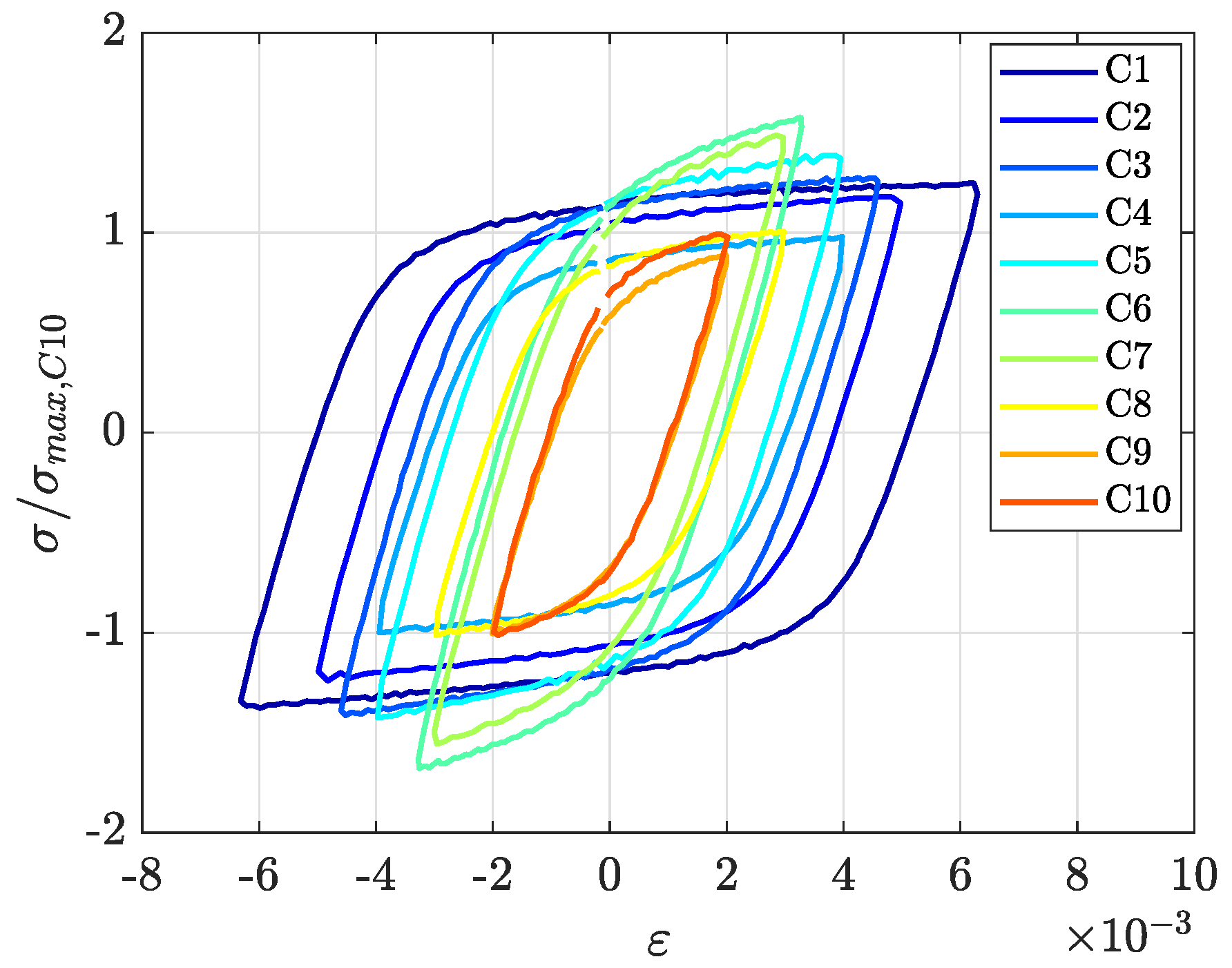
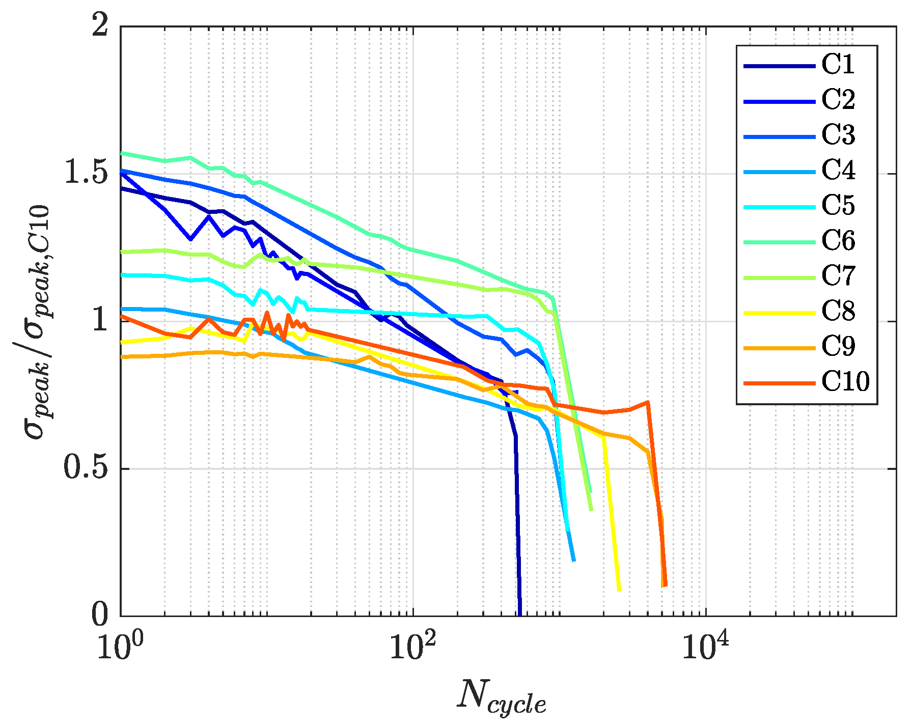
The midlife hysteresis cycles are reported, normalized to the maximum value of tensile stress of test C10, in Figure 4. The peak tensile stresses are reported in Figure 5, normalized with respect to the peak values of test C10.

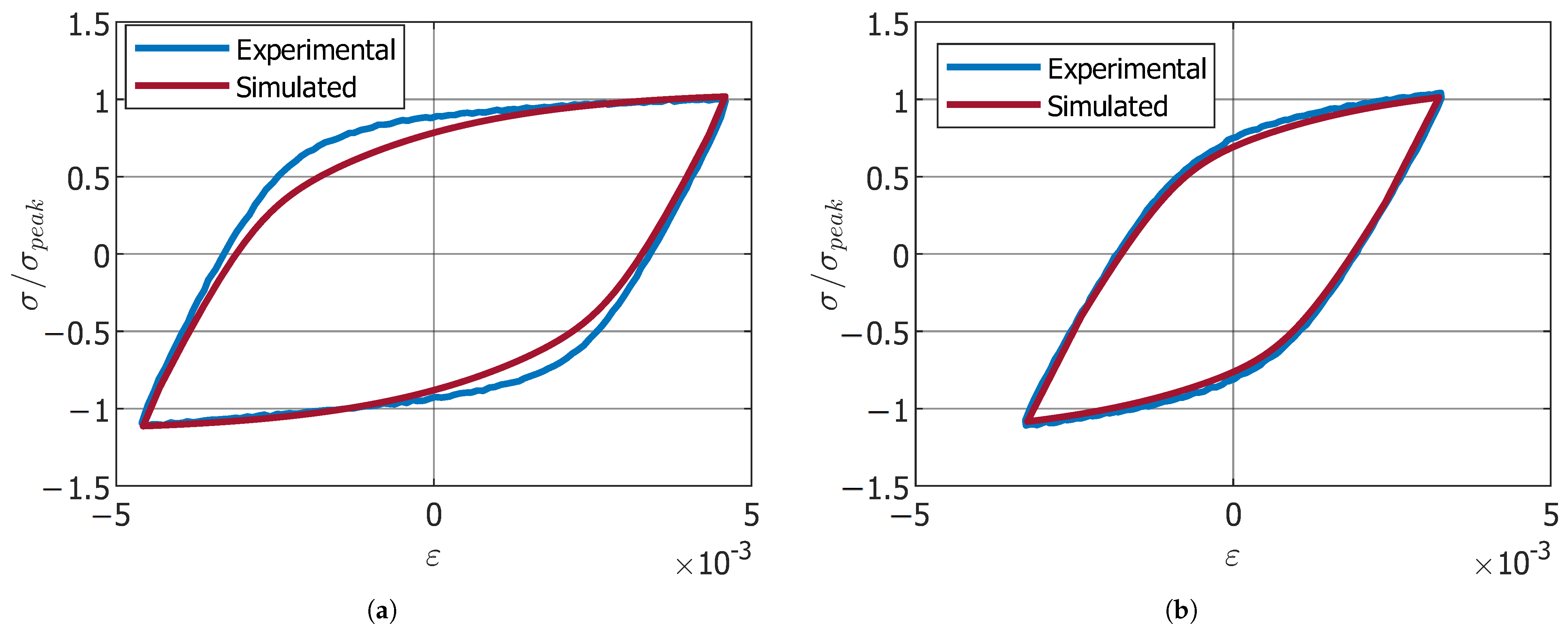
The comparison between the simulated hysteresis cycles and the two LCF tests used for parameter identification is shown in Figure 6. In Figure 7, the evolution of the peak tensile stress obtained from the simulation is compared with the experimental data up to midlife. For both figures, the y-axis is normalized to the respective peak tensile stress. The Chaboche–Voce parameters obtained provide a satisfactory representation of the stabilized cyclic response of the material.

Regarding the LCF damage model (Section 2.2.3), the relationship between the alternating plastic strain, ${\epsilon }_{pl,alt}$, and the peak tensile stress, ${\sigma }_{peak}$, for the LCF test at $\mathsf{\Delta }\epsilon =1.20\%$ and 500 °C is shown in Figure 8. The red points represent the data used for fitting with a second-degree polynomial. The stress range between 150 MPa and 300 MPa encompasses approximately 80% of the LCF life prior to macrocrack formation, indicating that the fit is satisfactory.

The peak tensile stress, ${\sigma }_{peak}$, was recorded throughout each test until the final drop associated with crack propagation. Using the relationship shown in Figure 8, it is possible to estimate the plastic strain accumulated during each cycle and, consequently, the corresponding value of $p_R$.

The same fitting procedure and calculation of $p_R$ were applied to all available LCF tests. The plastic strain rate, $\dot{p}$, was calculated by dividing $p_R$ by the test duration. The results are summarized in

Table 5. Results from testing campaign necessary to identify Kachanov-based LCF damage model parameters.

$\mathbf{\Delta }\mathit{\epsilon }(\%)$	${\mathit{N}}_{\mathit{R}}$	${\mathit{p}}_{\mathit{R}}$	$\dot{\mathit{p}}·{10}^3(1/\mathit{s})$	$\mathit{t}\left(\mathit{h}\right)$
1.20	537	10.4	2.639	1.096
1.00	599	8.5	$3.38$	0.700
0.90	1060	13.5	$2.09$	1.800
0.80	1251	12.1	$2.810$	1.200
0.80	1131	10.9	$3.03$	1.00
0.65	1616	10	$1.380$	2.01
0.60	2559	17.9	$3.54$	1.401
0.60	1647	8.4	$2.610$	0.900
0.40	5091	22.9	$1.720$	3.70
0.40	5305	20.9	$1.630$	3.56

.

In order to evaluate ${\varphi }_p$, given the hysteresis cycle that occurs at midlife, in Equation (21), the value of p introduced is half of $p_R$, and $\tilde{E}$ is calculated from elastic unloading after the peak under tensile conditions at the midlife cycle. The other two model parameters left, $M_p$ and ${\chi }_p$, are evaluated by fitting the experimental points $p_R\left(\dot{p}\right)$ with Equation (18), as it can be seen in Figure 9.

For the investigated material and the conducted testing campaign, the values of the LCF damage model parameters are reported in Table 6, including the variability range for the parameter $M_p$.

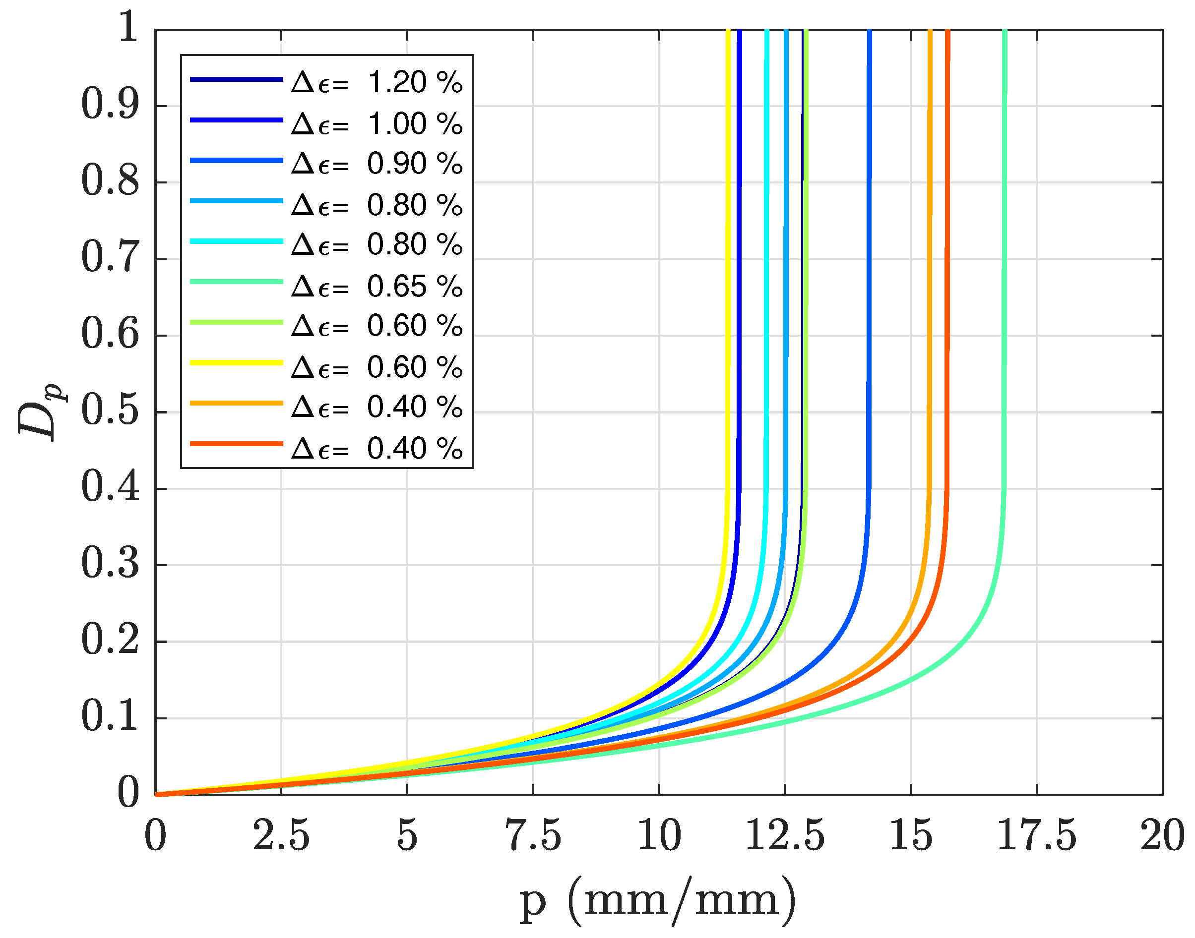
The resulting damage curves, obtained using Equation (17) with the parameters from Table 6 and the mean accumulated plastic strain rates reported in Table 5, are presented in Figure 10.

The evolution of damage is nonlinear, with the slope of the curve increasing sharply as p approaches $p_R$. The damage value at half of $p_R$ remains very small, in agreement with the experimental damage estimated from the softened elastic modulus. The maximum estimated $p_R$ ranges between 10 and 17.5, according to the regression results shown in Figure 9.

It should be noted that direct experimental validation of the trends in Figure 10 is challenging. The damage evolution presented in this study is derived from internal state variables within the constitutive model, which are not directly measurable in physical experiments. These variables represent microstructural degradation mechanisms that evolve during plastic deformation and are essential to predictive modeling, yet they do not correspond directly to observable quantities.

Indirect experimental verification is also difficult. While macroscopic indicators such as stiffness degradation, crack initiation, or changes in ductility can suggest damage accumulation, they do not provide a one-to-one correlation with the internal damage variable used in the model. Nevertheless, the model was calibrated and validated against macroscopic experimental data, including stress–strain curves and failure patterns, which indirectly support the plausibility of the damage evolution trends. These comparisons ensure that the model behaves consistently with observed physical phenomena, even though the internal variables themselves cannot be directly verified.

3.1.2. Creep and Creep Damage

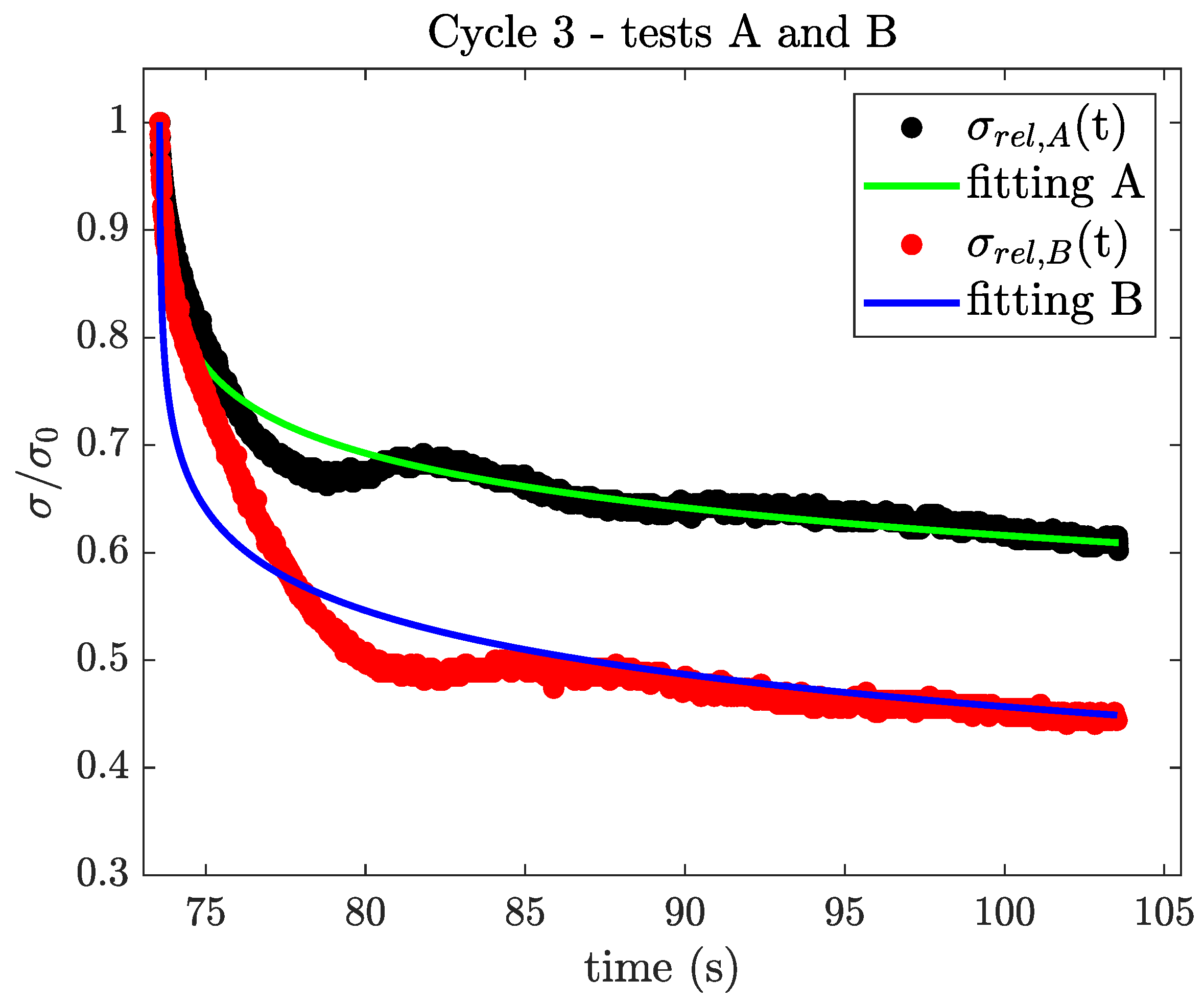
The Dorn secondary creep model was calibrated using the third hysteresis cycle of both LCF tests with hold time by fitting Equation (7) to the experimental data.

As shown in Figure 11, the Dorn secondary creep model accurately captures the stress relaxation behavior, with the simulated trends closely matching the experimental observations.

The parameters evaluated for the secondary creep model differ between the two stress trends. For the purposes of this study, the geometric mean of the two parameter sets was adopted as a reasonable compromise, as will be demonstrated later through numerical simulations. The numerical values of the Dorn secondary creep model (Equation (6)) are reported in Table 6.

The parameters of the sine-hyperbolic (SINH) creep damage model were determined through a two-step procedure. In the first step, the three parameters $Q_c$, ${\chi }_c$, and ${\sigma }_T$ were obtained by fitting the averaged values of $t_R\left(\sigma \right)$ from the data reported in [22] using Equation (10) within the operating stress range of the test campaign.

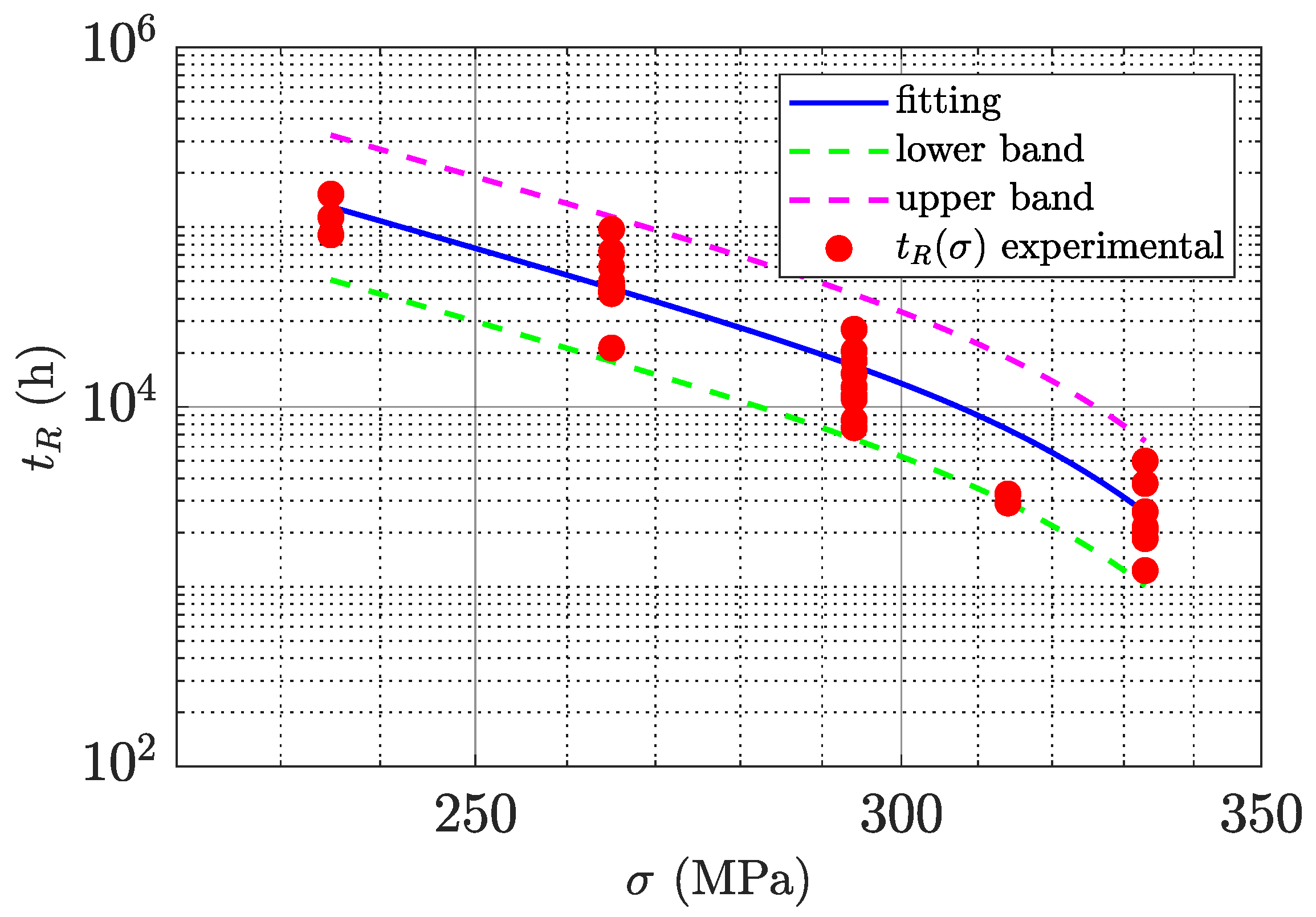
Figure 12 shows the rupture time data employed and the corresponding trend obtained from the implementation of Equation (10). The variability range of the parameter $Q_c$, reported in Table 6, is also represented by the lower and upper bounds indicated with dashed lines.

It can be observed that the function accurately represents the experimental data within the stress range of 235–333 MPa, which is relevant for the material investigated at 500 °C. The parameters obtained are listed in Table 6 and are used in Equation (10).

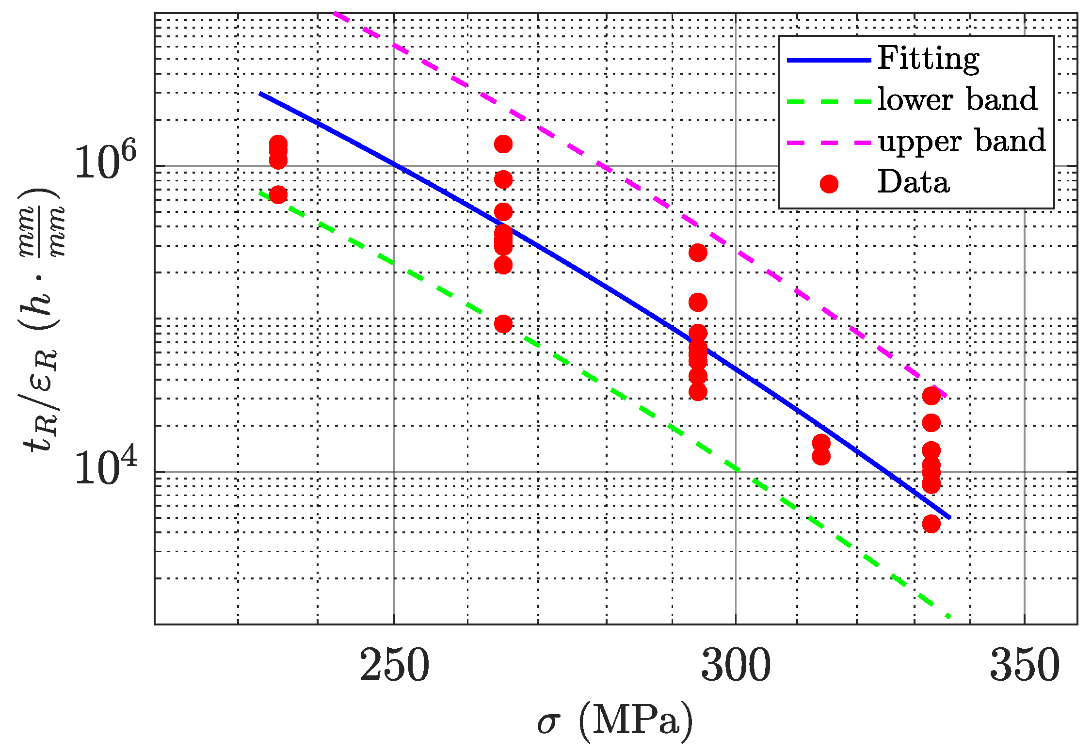
In the second step, after determining the first three parameters from the rupture time, the remaining pair of parameters, $\lambda$ and $\phi$, is obtained from Equation (13) using the NIMS data for the ratio $t_R/{\epsilon }_R$ versus $\sigma$, as summarized in Table 3. Figure 13 shows the ratio of rupture time to creep strain at failure and the corresponding trend obtained from the implementation of Equation (13).

The numerical values of $\lambda$ and $\phi$ are reported in Table 6. The upper and lower bounds plotted alongside the fitting curve correspond to the minimum and maximum values of $\phi$ listed in the same table.

The fitting exhibits a high degree of accuracy within the stress range of 265–333 MPa. However, at lower stress levels, there is a slight tendency to overestimate the ratio of $t_R/{\epsilon }_R$. Figure 14 presents the comparison between two simulated creep curves and the corresponding experimental data points.

3.1.3. Numerical Implementation

The various constitutive models exploited throughout the paper are summarized in Table 6, where all the parameters to be evaluated are shown, as well as their numerical value and the experimental quantities necessary for the fitting procedures.

Table 6. Parameters needed for the implementation of the proposed constitutive model.

Constitutive Models	Parameters	Fitting Requirements	Reference Figure
Elasticity	E = 170 GPa	At least one hysteresis cycle	Figure 3
Chaboche–Voce hardening	$C_1=40·{10}^3$ MPa $C_2=7$ MPa $C_3=600·{10}^3$ MPa ${\gamma }_1=474$ ${\gamma }_2=1$ ${\gamma }_3=3867$ $Q=-90$ MPa $b=1.130$ ${\sigma }_Y=125$ MPa	Two hysteresis cycles at midlife Stress peaks during LCF	Figure 6 and Figure 7
LCF Kachanov-like damage model	$M_p=6.89·{10}^{-2}$ ($s^{{\chi }_p}$) $M_p^{+}=15.4·{10}^{-2}$ ($s^{{\chi }_p}$) $M_p^{-}=0.02·{10}^{-2}$ ($s^{{\chi }_p}$) ${\chi }_p=0.418$ ${\varphi }_p=12.51$	Accumulated plastic strain to rupture $p_R$ Accumulated plastic strain rate $\dot{p}$ Softened elastic modulus at midlife	Figure 9
Dorn secondary creep	A = 1.223$·{10}^{-6}$ (h−1) B = 6.03$·{10}^{-2}$ (MPa−1)	Stress relaxation during hold-time for two cycles	Figure 11
Creep SINH damage model	$Q_c=4.52·{10}^{-5}$ (h−1) $Q_c^{+}=5.03·{10}^{-5}$ (h−1) $Q_c^{-}=3.14·{10}^{-5}$ (h−1) ${\chi }_c=8.16$ ${\sigma }_T=292$ MPa $\phi =-12.40$ ${\phi }^{+}=-11.40$ ${\phi }^{-}=-12.50$ $\lambda =11.20$ $r=1$	Time to rupture $t_R\left(\sigma \right)$ Creep-rupture strain ${\epsilon }_R\left(\sigma \right)$	Figure 12 and Figure 13

Table 6. Parameters needed for the implementation of the proposed constitutive model.

Constitutive Models	Parameters	Fitting Requirements	Reference Figure
Elasticity	E = 170 GPa	At least one hysteresis cycle	Figure 3
Chaboche–Voce hardening	$C_1=40·{10}^3$ MPa $C_2=7$ MPa $C_3=600·{10}^3$ MPa ${\gamma }_1=474$ ${\gamma }_2=1$ ${\gamma }_3=3867$ $Q=-90$ MPa $b=1.130$ ${\sigma }_Y=125$ MPa	Two hysteresis cycles at midlife Stress peaks during LCF	Figure 6 and Figure 7
LCF Kachanov-like damage model	$M_p=6.89·{10}^{-2}$ ($s^{{\chi }_p}$) $M_p^{+}=15.4·{10}^{-2}$ ($s^{{\chi }_p}$) $M_p^{-}=0.02·{10}^{-2}$ ($s^{{\chi }_p}$) ${\chi }_p=0.418$ ${\varphi }_p=12.51$	Accumulated plastic strain to rupture $p_R$ Accumulated plastic strain rate $\dot{p}$ Softened elastic modulus at midlife	Figure 9
Dorn secondary creep	A = 1.223$·{10}^{-6}$ (h−1) B = 6.03$·{10}^{-2}$ (MPa−1)	Stress relaxation during hold-time for two cycles	Figure 11
Creep SINH damage model	$Q_c=4.52·{10}^{-5}$ (h−1) $Q_c^{+}=5.03·{10}^{-5}$ (h−1) $Q_c^{-}=3.14·{10}^{-5}$ (h−1) ${\chi }_c=8.16$ ${\sigma }_T=292$ MPa $\phi =-12.40$ ${\phi }^{+}=-11.40$ ${\phi }^{-}=-12.50$ $\lambda =11.20$ $r=1$	Time to rupture $t_R\left(\sigma \right)$ Creep-rupture strain ${\epsilon }_R\left(\sigma \right)$	Figure 12 and Figure 13

Once all the necessary model parameters have been evaluated, the constitutive models are numerically implemented according to the algorithm shown in Figure A1.

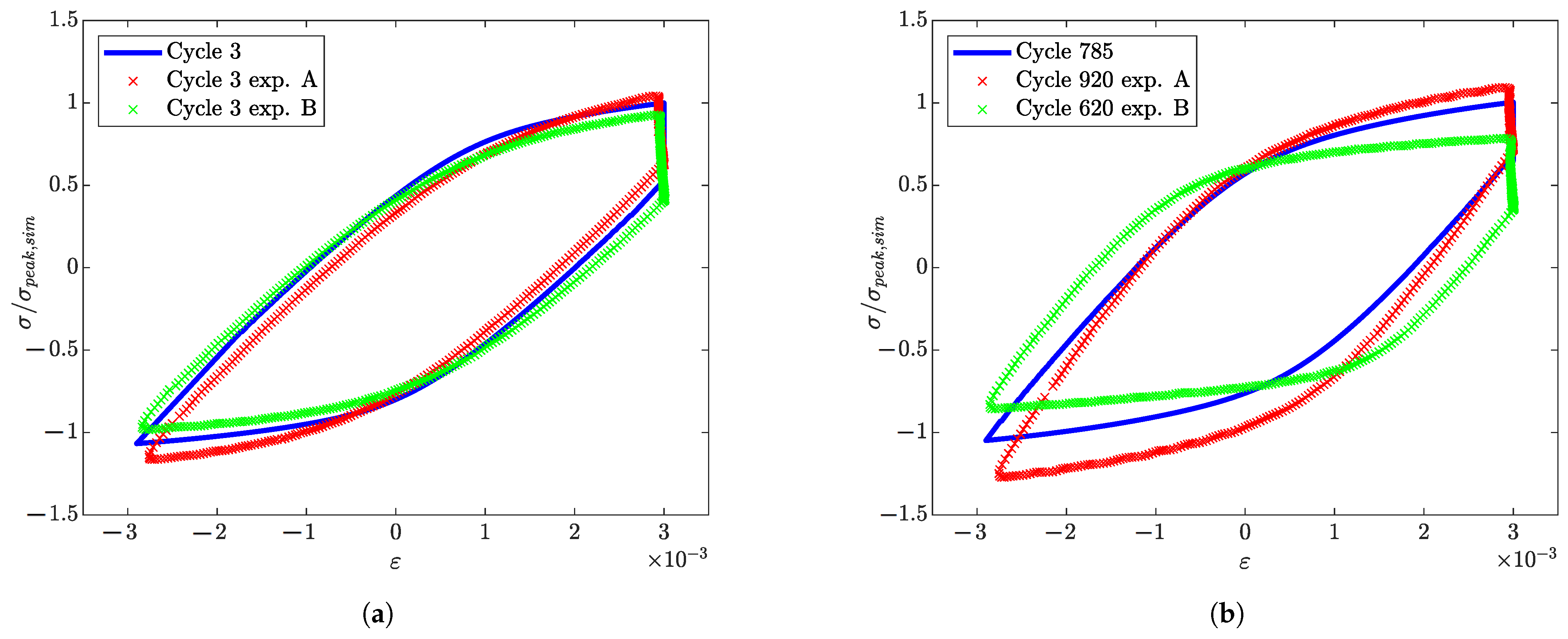
Figure 15 and Figure 16 show the comparison between simulated cycles and the experimental ones (the third cycle and the midlife cycle are represented). The y-axis in the two graphs are normalized to the respective simulated peak tensile stress. It is possible to see that the simulated cycles are adapted in coherence with the experimental variability of the shape of the cyclic stress–strain curve.

The comparison was performed at midlife to emphasize the correspondence between the model and the experiments when a comparable damage level is reached. Although it would also be informative to compare the cycle shape at exactly the same number of cycles, for the purposes of this study, it was considered more meaningful to compare the cycles for the same damage condition.

The amount of stress relaxed at the beginning of the cycling is approximately the same as observed experimentally, whereas at midlife, it is slightly lower than the experimental values. This level of approximation may be acceptable for conservative predictions, particularly when focusing on component reliability.

While the elastic moduli are similar at the third cycle, a more pronounced difference is observed at midlife. This discrepancy may result from variations in damage evolution for the same material under identical temperature, total strain range, and hold-time conditions.

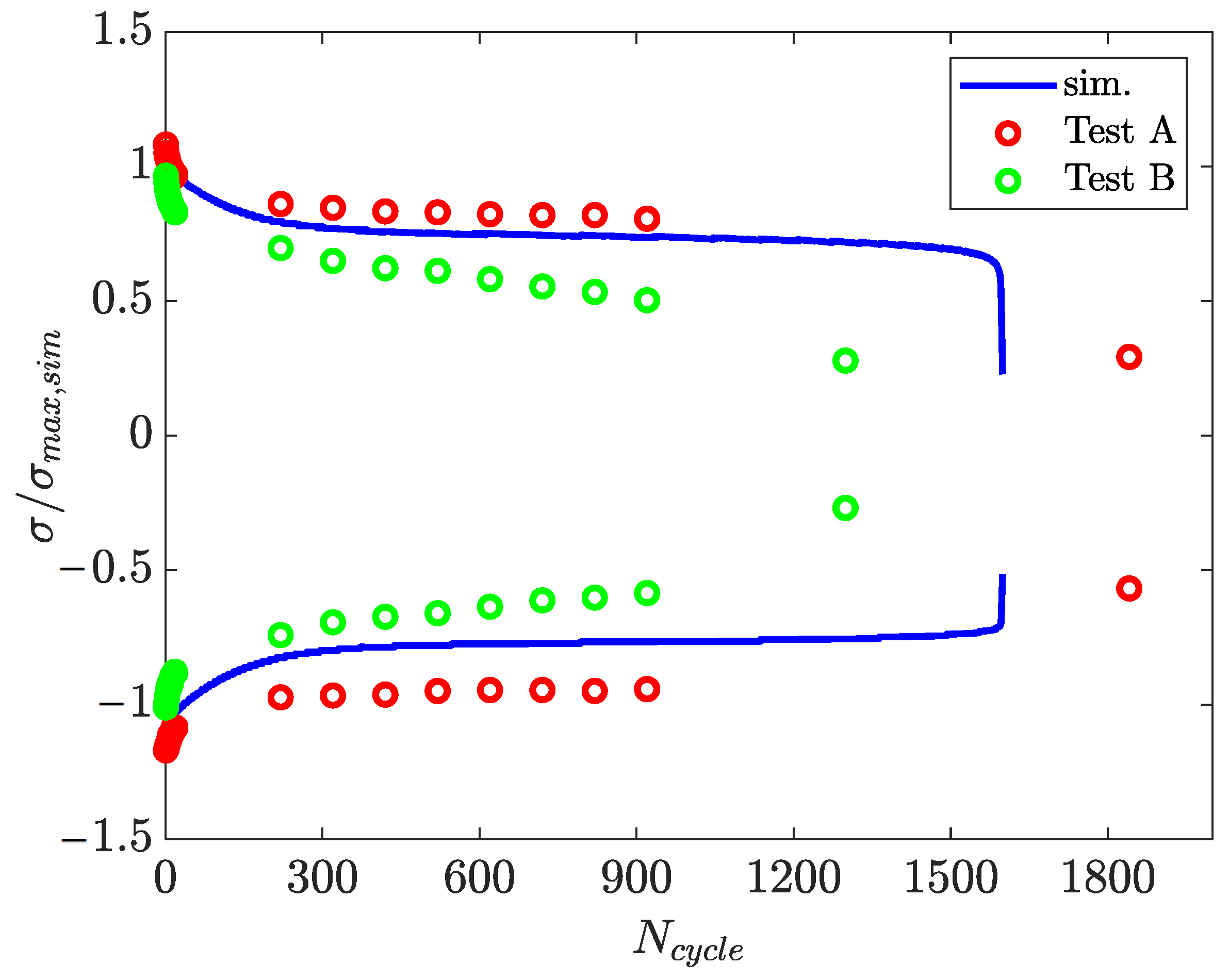
Figure 16 highlights another noteworthy aspect: the reduction in the positive ${\sigma }_{peak}$. Both tested cycles exhibit a smooth decrease in peak stress, suggesting the potential introduction of a term linearly dependent on p in the Voce isotropic hardening model, as previously discussed in [40]. The final simulated ${\sigma }_{peak}$ closely matches the experimental values, while the compressive ${\sigma }_{peak}$ aligns more closely with one of the two tests. A more detailed discussion of the discrepancies between simulations and experimental data is provided in Section 3.4.

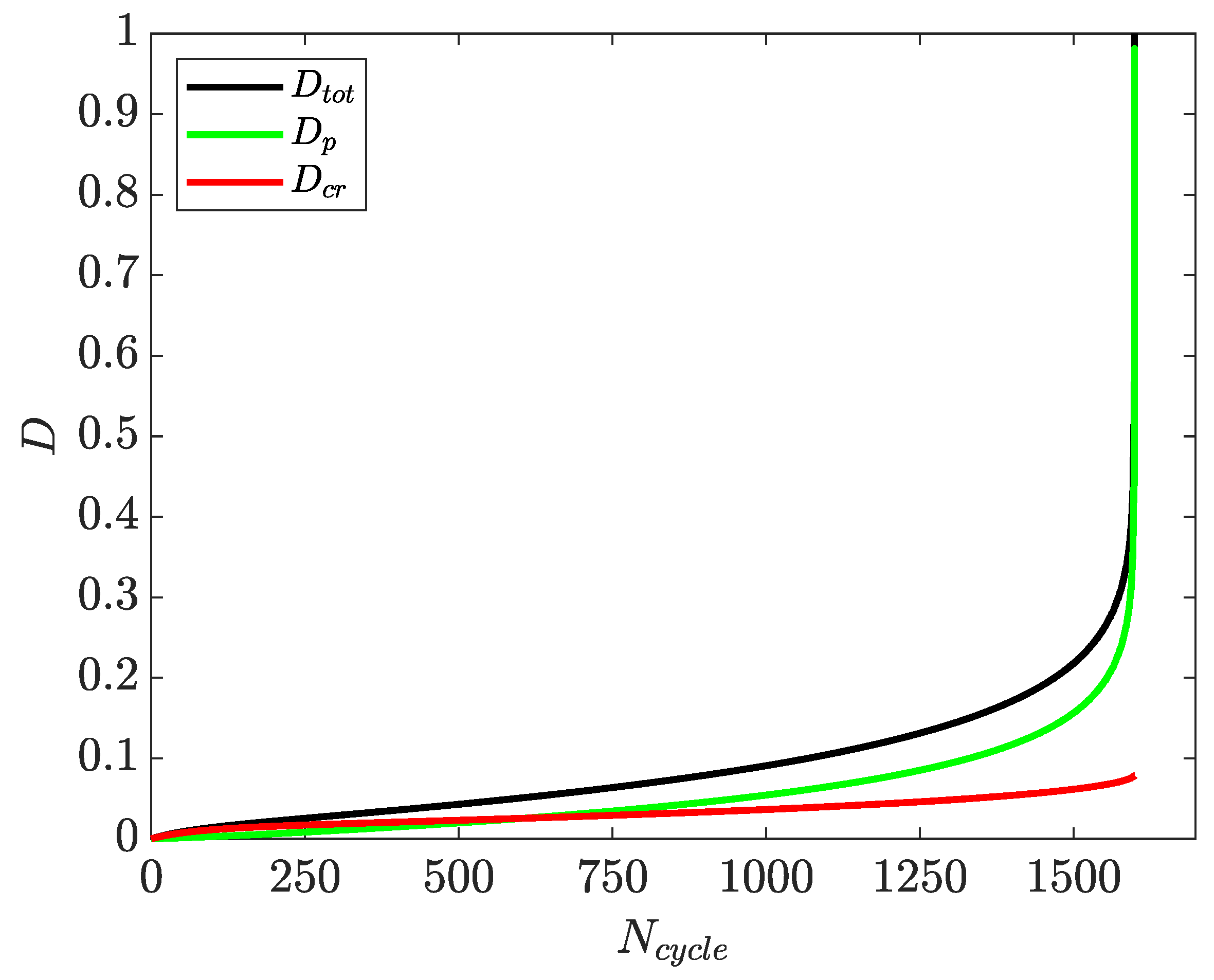
In Figure 17 the creep damage and LCF damage are plotted as functions of the number of cycles ($N_{cycle}$), as well as the total damage.

At the beginning of the test, creep damage saturates due to the reduction in stress resulting from isotropic hardening. However, towards the end of the cycling, the slope of the damage curve increases due to interaction with LCF damage. Plastic damage is significantly higher than creep damage, indicating that the presented test is primarily a fatigue-dominated test, accelerated by the creep occurring during the hold-time phases.

The cumulative fatigue damage up to midlife remains low, consistent with the tuning of ${\varphi }_p$ in Equation (21). The total damage, $D_{tot}$, is calculated as the linear sum of fatigue and creep damage, as stated in Equation (23). The influence of creep damage is the most pronounced during the initial cycles.

3.2. Validation

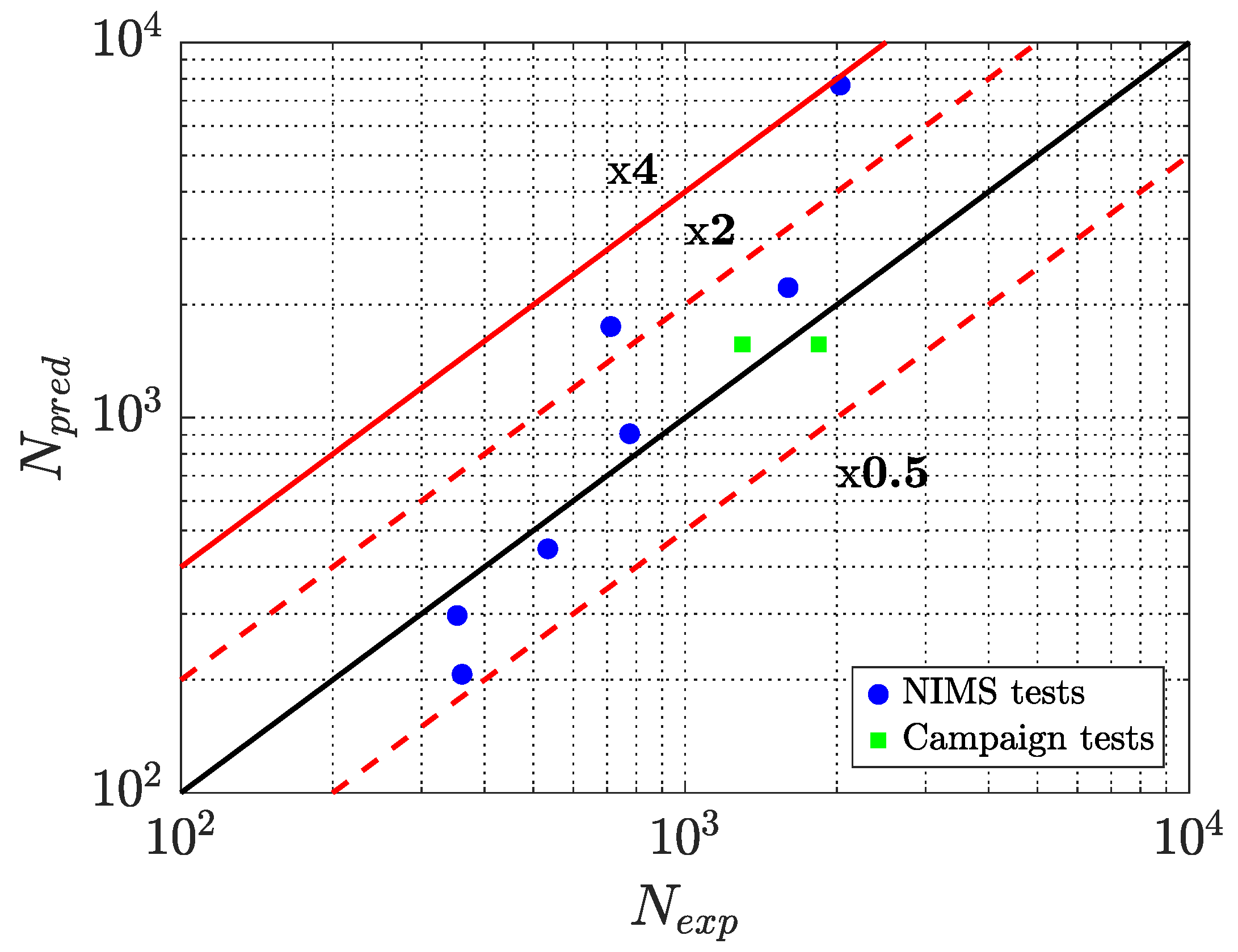
As mentioned in Section 2.1.1, for validation purposes, simulations were performed for different values of $\mathsf{\Delta }\epsilon /2$ and $t_H$, based on the experimental data reported in [21,22]. The predicted number of cycles to rupture, $N_{pred}$, was then compared with the experimental values, $N_{exp}$. The results are summarized in

Table 7. Comparison between experimental and predicted number of cycles to failure.

${\mathit{t}}_{\mathit{H}}\left(\mathit{s}\right)$	$\mathbf{\Delta }\mathit{\epsilon }$ / 2	${\mathit{N}}_{\mathit{exp}}$	${\mathit{N}}_{\mathit{pred}}$
30	0.30%	1841	1569
30	0.30%	1299	1569
360	1.02%	353	297
360	0.71%	776	906
360	0.50%	1600	2230
3600	1.02%	361	207
3600	0.81%	534	447
3600	0.51%	712	1750
3600	0.30%	2030	7703

.

The predicted number of cycles is of the same order of magnitude as the experimental results for nearly all reproduced conditions. The differences between the numerical simulations and the experimental data are illustrated in Figure 18, where the red dotted lines indicate factors of 0.5 and 2 and the solid line represents a larger factor.

Most simulations fall within the scatter band defined by factors of 0.5 and 2. The point exhibiting the largest deviation from the identity line is approximately near the line of the factor of 4. This notable discrepancy in predicted life can be attributed to the limitations of the creep damage model in accurately representing damage accumulation at low stress levels. The availability of additional experimental data would facilitate the identification of this limitation and support the development of creep damage models that do not rely solely on the current stress value.

Figure 18 shows that the simulated number of cycles is conservative for higher $\mathsf{\Delta }\epsilon$ values, whereas it slightly underestimates life at lower $\mathsf{\Delta }\epsilon$. This level of scatter is comparable to that typically observed when using assessment procedures directly aligned with standards such as the ASME BPVC or R5. Such results are characteristic of the creep–fatigue domain, particularly when new methodologies are tested. Relevant findings on this topic are presented in [10,11,13,14,28,41], with comparable quality results reported in [42].

It should be emphasized that the methodology presented here, within the context of industrial asset management (such as steam or gas turbine rotors), is suitable for predicting the response under complex loading cycles due to its algorithmic framework, which accounts for the combined evolution of stress and temperature over time, as described in the previous sections.

When addressing complex loading conditions, several simplifying assumptions are typically adopted to ensure a conservative approach in accordance with existing standards for creep–fatigue life prediction. Additionally, approaches such as the bilinear lifting method are primarily based on standard hold-time tests. While these criteria perform adequately under such scenarios, their applicability to complex, service-like loading cycles requires further evaluation. Consequently, future investigations should focus on testing the methodology proposed herein under realistic, service-like rotor loading conditions to assess its predictive capability in these more demanding applications.

Another important aspect to highlight is the relatively limited number of tests required to feed the model. Overall, a standard isothermal testing campaign, complemented by a few hold-time isothermal tests (provided that an adequate creep characterization is available), is sufficient to apply the methodology presented herein.

3.3. Analysis of Sensitivity to Hold Time

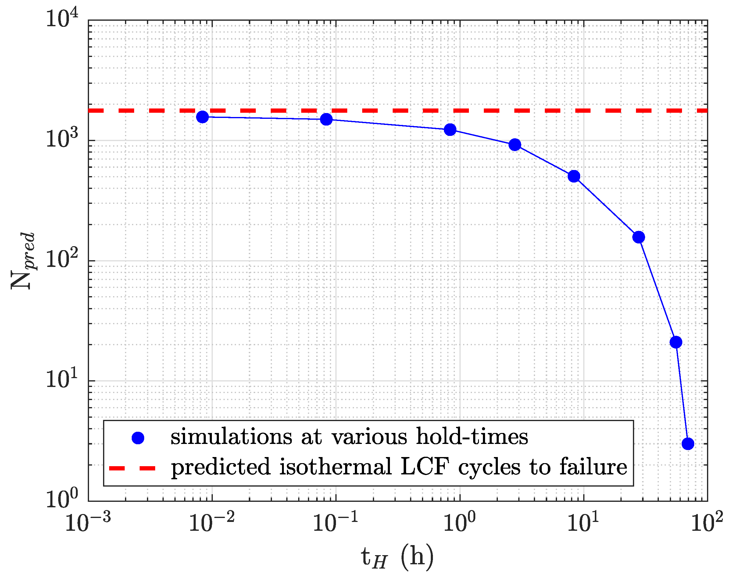
The effect of the hold-time variable was investigated by running the model multiple times at a fixed strain range. Specifically, simulations were performed at $\mathsf{\Delta }\epsilon /2=0.60\%$ with hold-time values spanning several orders of magnitude. The results, presented in Figure 19, show the number of cycles to failure as a function of the hold time, compared with the predicted number of cycles to failure obtained from isothermal LCF testing (red dotted line).

As demonstrated in Figure 19, hold-time values in excess of 6 minutes (i.e., ${10}^{-1}$ h) exert a substantial influence on the number of cycles of the material. In instances where the hold time exceeds 1 hour, the predicted number of cycles approaches less than half of the pure LCF life. The trend shown reflects the fact that creep damage rapidly accumulates when increasing the hold-time value.

It should also be remarked that usually, test data and prediction by more conventional approaches show saturation of life at long hold times as stress continues to relax. A possible interpretation of the behavior shown at high hold-time values is given by the fact that the damage accumulation rate is currently driven by the prediction of time to rupture fed by the NIMS data. A low relaxation rate combined with a too-high predicted damage accumulation rate might result in the lack of a second horizontal asymptotic behavior. It is also realistic that increasing the number of simulation points should show a saturation value. However, this aspect was not considered of interest for this specific paper and for the current industrial application of the model (directed mostly towards a high number of cycle applications with limited hold-time values). The calibration of the model with more accurate data, directed towards applications with longer hold times, would probably result in the observation of these kinds of phenomena.

3.4. Critical Review of Model Limitations and Testing Campaign Adequacy

When evaluating the overall performance of the model against the raw experimental data, it should be emphasized that the results presented are closely linked to the specific procedure used for parameter derivation. In the context of applying this methodology to industrial assets, a preliminary assumption was the availability of only a limited dataset of low-cycle fatigue (LCF) tests with hold time. If such a dataset is available, many of the steps outlined in the Materials and Methods Section can be bypassed, enabling the fitting procedure to be performed directly on the available hold-time tests. This fitting can be carried out using a variety of approaches, including modern techniques based on artificial intelligence, to achieve a faster and more efficient process. Therefore, the results shown in Figure 18, including both the lower- and higher-accuracy points, can be interpreted as the outcome of applying the proposed parameter-tuning methodology.

On the other hand, looking at more specific aspects, the testing campaign was also characterized by some peculiarities: Tests performed at the same temperature and delta strain range as presented in Figure 15 showed diversity in their response, including the cyclic hardening behavior, as can be seen from Figure 16. Test B saturates quickly after around 200 cycles, while Test A continues showing a more significant hardening behavior.

The model proposed here, calibrated using LCF and creep data, exhibits an early hardening behavior that more closely resembles Test A. This observation indicates that the cyclic deformation behavior of the material is more complex than assumed by the current models. Expanding the experimental campaign would likely provide a deeper understanding of the hardening mechanisms, which could be addressed, for instance, by incorporating a more complex dependence of the model parameters on the accumulated strain. Nonetheless, the results obtained for the present campaign appear promising and insightful.

Table 7 reports results for different hold times; however, it should be acknowledged that the trends are not immediately evident due to data scatter, particularly for Tests A and B. This variability likely reflects the inherent response heterogeneity of the material under creep–fatigue conditions, which can be influenced by factors such as microstructural inhomogeneity, oxidation, and testing conditions. Specifically, while an increase in hold-time generally corresponds to a reduction in the number of cycles to failure (Figure 19), consistent with increased creep damage accumulation, the observed scatter prevents a definitive quantitative conclusion.

It should also be noted that a more extensive experimental campaign, encompassing a greater number of creep–fatigue tests, higher variability, longer hold times, and additional repetitions, would support validation of the methodology under conditions beyond those currently investigated. Increased data availability would enable a more thorough assessment of test variability and provide the opportunity to evaluate the model’s predictive capability under longer hold times or variable temperature conditions.

Future work will also focus on comparing the methodology proposed herein with more conventional approaches for creep–fatigue life prediction.

4. Conclusions

The main outcomes of the proposed model and its associated analyses can be summarized and commented as follows:

• A model for creep–fatigue interaction has been developed and applied to a martensitic steel alloy operating at 500 °C. The novelty of the model lies in the introduction of an LCF damage accumulation formulation inspired by the Kachanov–Rabotnov creep damage approach.
• The more advanced sine-hyperbolic constitutive model for creep damage is employed as a companion to the proposed LCF damage model.
• A systematic procedure for identifying the parameters of secondary creep, creep damage, and LCF damage models is presented. For the time-independent plasticity component, conventional but reliable nonlinear hardening models are retained. Overall, the proposed procedure appears practical and manageable within an industrial context, even when a relatively large number of input parameters is required.
• Numerical simulations were performed for the two LCF tests with a 30 s hold time, as well as for additional loading conditions for validation purposes. The predicted life values were compared to experimental data, and the simulations fall within an acceptable error range for industrial prediction purposes.

It should be emphasized that the full potential of this methodology is expected to emerge when applied to complex loading histories involving simultaneous variations in temperature and strain, where conventional approaches often become overly conservative, resulting in excessive design and operational margins for turbomachinery components. This highlights the relevance and interest of the present research within the industrial sector.

References

1. Bucciarelli, F.; Checcacci, D.; Girezzi, G.; Signorini, A. Steam Turbines Subject to Frequent Start by Rotor Stress Monitoring. In Proceedings of the ASME Turbo Expo, Virtual, 21–25 September 2020. [Google Scholar] [CrossRef]
2. Dettori, S.; Maddaloni, A.; Galli, F.; Colla, V.; Bucciarelli, F.; Checcacci, D.; Signorini, A. Steam Turbine Rotor Stress Control through Nonlinear Model Predictive Control. Energies 2021, 14, 3998. [Google Scholar] [CrossRef]
3. Garrucciu, V.; Bacci di Capaci, R.; Vaccari, M.; Manara, S.; Bucciarelli, F.; Signorini, A.; Pannocchia, G. Efficient NMPC strategies for thermal stress control of steam turbines. IFAC-PapersOnLine 2024, 58, 29–34. [Google Scholar] [CrossRef]
4. Holdsworth, S. Creep-Fatigue Failure Diagnosis. Materials 2015, 8, 7757–7769. [Google Scholar] [CrossRef]
5. Gariboldi, E.; Spigarelli, S. High-Temperature Behavior of Metals. Metals 2021, 11, 1128. [Google Scholar] [CrossRef]
6. Saxena, A. A Phenomenological Model for Creep and Creep-Fatigue Crack Growth Rate Behavior in Ferritic Steels. Metals 2023, 13, 1749. [Google Scholar] [CrossRef]
7. Sidey, D. Some interactions between creep and fatigue in a 1% Cr Mo V steel. Mater. Sci. Eng. 1978, 33, 189–197. [Google Scholar] [CrossRef]
8. American Society of Mechanical Engineers. ASME Boiler & Pressure Vessel Code, Section III, Division 1, Subsection NH, Rules for Construction of Nuclear Facility Components; American Society of Mechanical Engineers: New York, NY, USA, 2021. [Google Scholar]
9. British Energy. R5: Assessment Procedure for the High Temperature Response of Structures; Springer Nature: Gloucester, UK, 2003; Issue 3. [Google Scholar]
10. Lemaitre, J.; Desmorat, R. Engineering Damage Mechanics, 1st ed.; Springer: Berlin/Heidelberg, Germany, 2005; pp. 45–52. [Google Scholar]
11. Lemaitre, J.; Chaboche, J.L. Mechanics of Solid Materials, 3rd ed.; Cambridge University Press: Cambridge, UK, 2000; pp. 161–449. [Google Scholar]
12. Sen, S.; Almstedt, H. Constitutive Model based efficient creep-fatigue damage computation technique for steam turbine rotor to enhance flexible operational capabilities. In Proceedings of the ASME Turbo Expo, Boston, MA, USA, 26–30 June 2023. [Google Scholar]
13. Shigeyama, H.; Takahashi, Y.; Siefert, J.; Parker, J. Creep-Fatigue Life Evaluation for Grade 91 Steels with Various Origins and Service Histories. Metals 2024, 14, 148. [Google Scholar] [CrossRef]
14. Wang, X.; Zhang, W.; Zhang, T.; Gong, J.; Abdel Wahab, M. A New Empirical Life Prediction Model for 9–12% Cr Steels under Low Cycle Fatigue and Creep Fatigue Interaction Loadings. Metals 2019, 9, 183. [Google Scholar] [CrossRef]
15. Zhang, T.; Wang, X.; Zhang, W.; Hassan, T.; Gong, J. Fatigue–Creep Interaction of P92 Steel and Modified Constitutive Modelling for Simulation of the Responses. Metals 2020, 10, 307. [Google Scholar] [CrossRef]
16. Jürgens, M.; Olbricht, J.; Fedelich, B.; Skrotzki, B. Low Cycle Fatigue and Relaxation Performance of Ferritic–Martensitic Grade P92 Steel. Metals 2019, 9, 99. [Google Scholar] [CrossRef]
17. Mroziński, S.; Lis, Z.; Egner, H. Influence of Creep Damage on the Fatigue Life of P91 Steel. Materials 2022, 15, 4917. [Google Scholar] [CrossRef] [PubMed]
18. Holdsworth, S.R.; Mazza, E.; Binda, L.; Ripamonti, L. Development of thermal fatigue damage in 1CrMoV rotor steel. Nucl. Eng. Des. 2007, 237, 2292–2301. [Google Scholar] [CrossRef]
19. Cui, L.; Wang, P.; Hoche, H.; Scholz, A.; Berger, C. The influence of temperature transients on the lifetime of modern high-chromium rotor steel under service-type loading. Mater. Sci. Eng. A 2013, 560, 767–780. [Google Scholar] [CrossRef]
20. Abe, F.; Kern, T.U.; Viswanathan, R. Creep-Resistant Steels, 1st ed.; Woodhead Publishing Limited: Cambridge, UK, 2008; pp. 573–593. [Google Scholar]
21. Furuya, Y.; Nishikawa, H.; Hirukawa, H.; Nagashima, N.; Takeuchi, E. Catalogue of NIMS fatigue data sheets. Sci. Technol. Adv. Mater. 2019, 20, 1055–1072. [Google Scholar] [CrossRef] [PubMed]
22. Sawada, K.; Kimura, K.; Abe, F.; Taniuchi, Y.; Sekido, K.; Nojima, T.; Watanabe, T. Catalogue of NIMS creep data sheets. Sci. Technol. Adv. Mater. 2019, 20, 1131–1149. [Google Scholar] [CrossRef] [PubMed]
23. Tamura, M.; Abe, F.; Shiba, K.; Sakasegawa, H.; Tanigawa, H. Larson–Miller Constant of Heat-Resistant Steel. Metall. Mater. Trans. A 2013, 44, 2645–2661. [Google Scholar] [CrossRef]
24. Maruyama, K.; Abe, F.; Sato, H.; Shimojo, J.; Sekido, N.; Yoshimi, K. On the physical basis of a Larson-Miller constant of 20. Int. J. Press. Vessel. Pip. 2018, 159, 93–100. [Google Scholar] [CrossRef]
25. Guštin, A.Z.; Žužek, B.; Podgornik, B. Creep Life Prediction of 10CrMo9–10 Steel by Larson–Miller Model. Materials 2022, 15, 4431. [Google Scholar] [CrossRef]
26. Stewart, C.M. A Hybrid Constitutive Model for Creep, Fatigue and Creep-Fatigue Damage. Ph.D. Thesis, University of Central Florida, Orlando, FL, USA, 2013. [Google Scholar]
27. Cui, L.; Wang, P. Two lifetime estimation models for steam turbine components under thermomechanical creep–fatigue loading. Int. J. Fatigue 2014, 59, 129–136. [Google Scholar] [CrossRef]
28. Bartošák, M.; Horváth, J. A continuum damage coupled unified viscoplastic model for simulating the mechanical behaviour of a ductile cast iron under isothermal low-cycle fatigue, fatigue-creep and creep loading. Int. J. Plast. 2024, 173, 103868. [Google Scholar] [CrossRef]
29. Santus, C.; Grossi, T.; Romanelli, L.; Pedranz, M.; Benedetti, M. A computationally fast and accurate procedure for the identification of the Chaboche isotropic-kinematic hardening model parameters based on strain-controlled cycles and asymptotic ratcheting rate. Int. J. Plast. 2023, 160, 103503. [Google Scholar] [CrossRef]
30. Mahmoudi, A.H.; Pezeshki-Najafabadi, S.M.; Badnava, H. Parameter determination of Chaboche kinematic hardening model using a multi objective Genetic Algorithm. Comput. Mater. Sci. 2011, 50, 1114–1122. [Google Scholar] [CrossRef]
31. Dvoršek, N.; Stopeinig, I.; Klančnik, S. Optimization of Chaboche Material Parameters with a Genetic Algorithm. Materials 2023, 16, 1821. [Google Scholar] [CrossRef] [PubMed]
32. Sattar, M.; Othman, A.R.; Kamaruddin, S.; Akhtar, M.; Khan, R. Limitations on the computational analysis of creep failure models: A review. Eng. Fail. Anal. 2022, 134, 105968. [Google Scholar] [CrossRef]
33. Kachanov, L.M.; Krajcinovic, D. Introduction to Continuum Damage Mechanics. J. Appl. Mech. 1987, 54, 481. [Google Scholar] [CrossRef]
34. Haque, M.S.; Stewart, C.M. Comparative analysis of the sin-hyperbolic and Kachanov–Rabotnov creep-damage models. Int. J. Press. Vessel. Pip. 2019, 171, 1–9. [Google Scholar] [CrossRef]
35. Liu, Y.; Murakami, S. Damage Localization of Conventional Creep Damage Models and Proposition of a New Model for Creep Damage Analysis. JSME Int. J. 1998, 41, 1. [Google Scholar] [CrossRef]
36. Hossain, M.A.; Haque, M.S.; Pellicotte, J.; Stewart, C.M. An advanced sine-hyperbolic creep-damage model incorporating threshold strength. In Proceedings of the ASME Turbo Expo, London, UK, 24–28 June 2024. [Google Scholar]
37. Pandey, V.B.; Singh, I.V.; Mishra, B.K. A Strain-based continuum damage model for low cycle fatigue under different strain ratios. Eng. Fract. Mech. 2021, 242, 107479. [Google Scholar] [CrossRef]
38. Chaboche, J.L. A review of some plasticity and viscoplasticity constitutive theories. Int. J. Plast. 2008, 24, 1642–1693. [Google Scholar] [CrossRef]
39. Rae, Y.; Benaarbia, A.; Hughes, J.; Sun, W. Experimental characterisation and computational modelling of cyclic viscoplastic behaviour of turbine steel. Int. J. Fatigue 2019, 124, 581–594. [Google Scholar] [CrossRef]
40. ANSYS® Theory Reference Manual, Release 2024R1; ANSYS Inc.: Canonsburg, PA, USA, 2024.
41. Kontermann, C.; Linn, S.; Oechsner, M. Application concepts and experimental validation of constitutive material models for creep-fatigue assessment of components. In Proceedings of the ASME Turbo Expo, Phoenix, AZ, USA, 17–21 June 2019. [Google Scholar]
42. Chen, F.; Zhang, W.; Zhang, K.; Yang, Q.; Wang, X.; Zhou, C. Low cycle fatigue and creep-fatigue interaction behavior of 2.25CrMoV steel at high temperature. J. Mater. Res. Technol. 2024, 28, 3155–3165. [Google Scholar] [CrossRef]
Figure 1. Mean value and dispersion range of LMP for different stress values at 500 °C.
Metals 15 01014 g001
Figure 2. Mean value and dispersion range of creep strain at rupture ε R for different stress values at 500 °C.
Metals 15 01014 g002
Figure 3. Third hysteresiscycle (normalized to peak tensile stress) of test C3 and prediction of Young’s modulus from elastic unloading under tensile conditions.
Metals 15 01014 g003
Figure 4. Hysteresis cycle at midlife for LCF tests at 500 °C. The y-axis is normalized to the peak tensile stress of the midlife hysteresis cycle of test C10.
Metals 15 01014 g004
Figure 5. σ p e a k normalized to the maximum peak tensile stress of test C10.
Metals 15 01014 g005
Figure 6. Comparison between tests and simulation, normalized to the respective peak tensile stress, of the hysteresis cycle for (a) Δ ε = 0.90 % and (b) Δ ε = 0.65 % .
Metals 15 01014 g006
Figure 7. Comparison between simulated and experimental peak stresses, normalized to the respective peak tensile stress, for Δ ε = 0.90 % and Δ ε = 0.65 % until midlife.
Metals 15 01014 g007
Figure 8. ε p l , a l t vs. σ p e a k (MPa) fitting for the test at Δ ε = 1.20 % and 500 °C.
Metals 15 01014 g008
Figure 9. p R ( p ˙ ) points obtained from testing campaign at various Δ ε at 500 °C.
Metals 15 01014 g009
Figure 10. LCF damage behavior as a function of accumulated plastic strain.
Metals 15 01014 g010
Figure 11. Stress relaxation during hold time t H = 30 s for Test A and Test B at the third cycle. The y-axis is normalized to the corresponding initial stress σ 0 of each test, that is, 300 MPa and 268 MPa for Tests A and B, respectively.
Metals 15 01014 g011
Figure 12. Creep-rupture data as a function of stress used to feed the model together with the trend of rupture time as predicted by the sine-hyperbolic model trend best fitting the available data.
Metals 15 01014 g012
Figure 13. Ratio of rupture time and creep strain to failure as a function of stress together with the trend of Equation (13) that best fits available data.
Metals 15 01014 g013
Figure 14. Comparison between simulation and experimental creep data at σ = 333 MPa and σ = 265 MPa. Adapted from refs. [21,22].
Metals 15 01014 g014
Figure 15. Comparison betweentests and simulation for (a) initial cycle and (b) midlife cycle. The two y-axes are normalized to the respective simulated σ p e a k under tensile conditions.
Metals 15 01014 g015
Figure 16. Comparison between σ p e a k under tension and compression conditions for the simulated and experimental cycles. The y-axis is normalized to the simulated maximum peak tensile stress.
Metals 15 01014 g016
Figure 17. Calculated D c r , D p , and D t o t .
Metals 15 01014 g017
Figure 18. Comparison between predicted ( N p r e d ) and experimental ( N e x p ) life. The red dotted lines are the bounds for the factors of 2 and 0.5, whereas the red solid line is the factor of 4. The black line is the identity line.
Metals 15 01014 g018
Figure 19. Simulated effect of the tH on a test with Δ ε / 2 = 0.60 % .
Metals 15 01014 g019