Modeling of Tensile Tests Flow Curves Using an Explicit Piecewise Inverse Approach

Abstract

Tensile tests are a common method for characterizing plastic behavior for sheet metal forming applications. During tensile testing at the beginning of the deformation, the stress state is uniaxial; however, as the deformation proceeds, the state changes to triaxial, making the post-processing of experimental data challenging using analytical methods. In contrast, inverse approaches in which the behavior is represented by constitutive equations and the parameters are fitted using an iterative procedure are extremely dependent on the empirical equation chosen at the outset and can be computationally expensive. The inverse piecewise flow curve determination method, previously developed for compression tests, is extended in this paper to tensile testing. A stepwise approach is proposed to calculate constant strain rate flow curves accounting for the unique characteristics of tensile deformation. To capture the effects of localized strain rate variations during necking, a parallel flow curve determination strategy is introduced. Tensile test flow curves for manganese-boron steel 22MnB5, a material commonly used in hot stamping applications, are determined, and the approach is demonstrated for virtual force–displacement curves. It has been shown that these curves can replicate the virtual experimental flow curves data with a maximum deviation of 1%.

1. Introduction and State of the Art

Tensile tests are fundamental for predicting work hardening behavior, though they face limitations due to the restricted range of homogeneous deformation compared to other testing methods. Specimens typically consist of a gauge section and two shoulders, with bulk materials using a rounded cross-section and sheet metals employing a flat rectangular cross-section [1,2]. During testing, the specimen is elongated until fracture, recording gauge length elongation (∆L) against the applied force (F). The resulting stress and strain values are termed engineering stress and strain, initially increasing linearly in the elastic regime before transitioning to nonlinearity due to work hardening [3].

After reaching maximum engineering stress, flow localization leads to plastic instability, known as diffusion necking, where deformation concentrates in a small region, causing a decrease in stress [3]. The elastic regime is minimal compared to overall plastic deformation, necessitating the transformation of the engineering stress–strain curve into a true stress–strain curve using established relationships. Hollomon’s power law [4] and the Ramberg–Osgood [5] equation are commonly employed to approximate these curves; however, extrapolating beyond necking often yields unreliable results, as these methods do not account for the change in the cross-sectional area [6]. Apart from the empirical equations to represent the flow curve, other metal physics based equations like the Kocks–Mecking model [7,8] or the 3IVM model [9] take into account strain hardening and softening processes by relating them to dislocation formation and annihilation. However, the material dependent parameters are not directly excluded but also must be obtained by using inverse methods. Furthermore, the number of these parameters is very large, and the inverse determination is complex and expensive [10].

Once diffusion necking initiates, the stress state becomes multiaxial, requiring transformation into equivalent stress and strain. Two primary approaches for determining flow curves post-necking exist, namely analytical methods using correction factors and inverse methods that iteratively adjust the flow curve to match experimental data. The correction factors based analytical methods, for example, the Bridgman correction factor [11] that is most widely used, which are based on the change in geometry of the necking specimen during deformation. A summary of different correction factors is given in [3,12]. The correction factors have a high dependency on the material and specimen geometry. It may be essential to tailor correction factors depending on the forming conditions [13]. The inverse methods, on the other hand, rely on predefined constitutive laws (e.g., Swift, Voce), which may not capture complex phenomena like dynamic recrystallization (DRX) or recovery (DRV) [14]. Advanced inverse techniques, such as the inverse finite element (FE) procedure based on DIC (IFD), improve accuracy but require extensive strain monitoring and are currently limited to flat specimens at room temperature [15].

Assessment of the Literature and the Problem Statement

The analytical methods described earlier either extrapolate the stress–strain data until necking, ignoring the actual stress state during diffusion necking, or use correction factors to obtain equivalent stress–strain curves. However, these correction factors are dependent on the gauge section geometry and also can be material-specific. In contrast, the conventional inverse methods are computationally expensive as well as rely on a predefined constitutive equation. Also, the piecewise inverse methods require additional continuous DIC monitoring of strain data and determine flow curves only at room temperatures.

Therefore, to overcome the above-mentioned limitations, this paper extends the inverse piecewise flow curve determination method—flow curve determination through explicit piecewise inverse modeling (FepiM)—previously developed by the present authors for hot compression tests [16,17] and torsion tests [18], and it is extended in this paper for tensile tests. The FepiM method is improved to address rapid changes in strain rate once necking begins, as the earlier consecutive stepwise approach cannot handle the post necking behavior. As a result, a parallel flow curve determination technique is used in this study to extend the established FepiM approach, with a particular focus on obtaining constant strain rate flow curves for tensile tests conducted at elevated temperatures. The following sections describe in detail the parallel flow curve determination methodology within the FepiM framework.

2. Materials and Methods

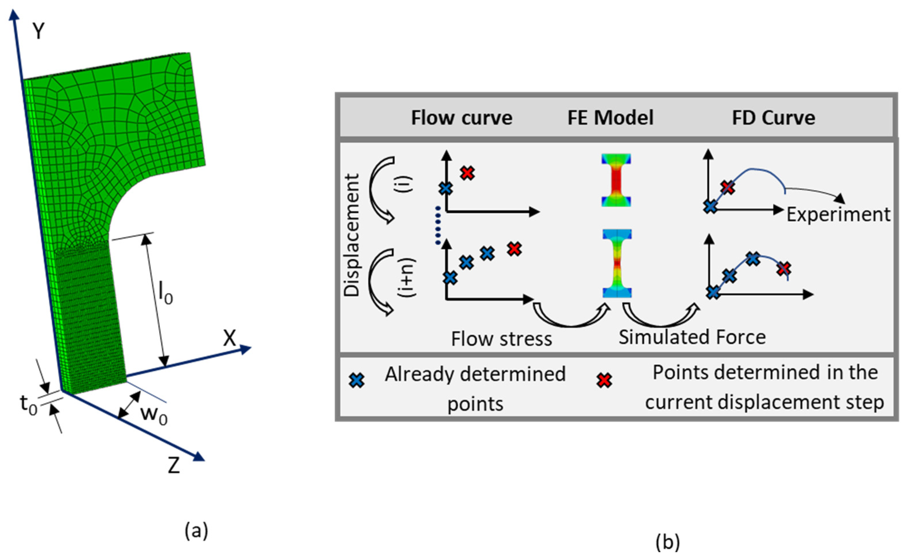
2.1. FE Model of the Tensile Specimen and Flow Curve Point Determination

The basis of an inverse pointwise flow curve determination is an FE model of the specimen. The tensile simulations were performed on rectangular cross-section flat tensile test specimens drawn from a sheet of thickness 1.5 mm. The specimen has an overall length of 59 mm, but the gauge section where most of the plastic deformation is concentrated has a width of 3 mm and length of 10 mm. The FE model (see Figure 1a) is developed in the commercial FE software Abaqus/Standard. Only one-eighth of the model is taken into account by considering the symmetries along the X, Y, and Z axes in the specimen, and it is meshed with 3D solid elements of type C3D8 (an 8-node linear thermally coupled brick element). A reference point is connected to the top surface that is parallel to the XZ plane, and a displacement is applied to this point along the Y-axis according to the experimental data.

Figure 1 also shows the illustration of the inverse approach and the consecutive flow curve point determination. Apart from the FE model, the initial flow stress of the material and the experimental force–displacement (FD) curve are also an input to FepiM. Initially, the FD curve is divided into different displacement steps, and a flow curve point is determined at each of these steps. For step (i) in Figure 1b, flow curve point (shown in red) is obtained such that at the corresponding displacement, the experimental and simulated forces match. To obtain a complete flow curve, this flow curve determination is then repeated at every displacement step in the FD curve until the final step. It should also be noted that once the flow curve point is determined, it remains the same and is not modified for the next displacement steps. The challenges corresponding to tensile tests and the exact approach for the flow curve determination approach are discussed in the next sections. Also, determining a flow curve point at every point on the FD curve can be computationally expensive, and therefore only some specific displacement steps are resampled from the experimental FD and are chosen based on the severity of the change in slope. These resampled points are called evaluation points (EPs), and the method to determine these points is discussed in [16].

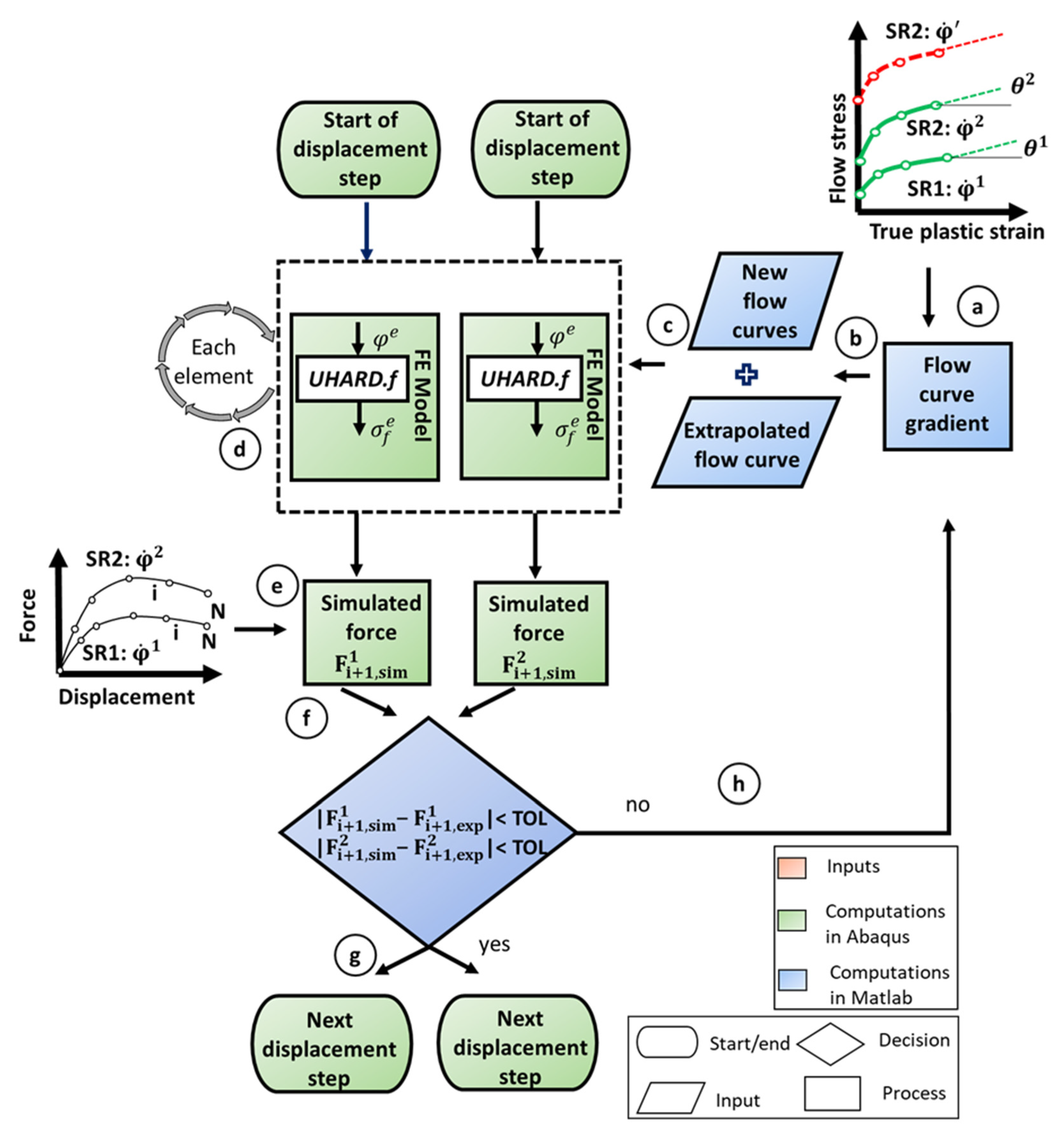
2.2. Constant Flow Curve Determination for Tensile Tests with FepiM

A parallel optimization approach is employed to determine tensile test flow curves at elevated temperatures with FepiM, where multiple flow curves corresponding to different strain rates are computed concurrently. Therefore, flow stress determination can also be performed during the necking phase by interpolating between stress data from higher strain rate flow curves. The detailed parallel optimization scheme is discussed below and illustrated in the flow diagram shown in Figure 2.

The flow diagram relates to an example where flow curves are simultaneously determined at nominal temperature T and at nominal strain rates of ${\dot{\phi }}^1$ and ${\dot{\phi }}^2$ (${\dot{\phi }}^1<{\dot{\phi }}^2$). Therefore, two FD curves representing experiments at two distinct strain rates are provided as input to FepiM in this scenario. These FD curves are divided such that they have the same number of EPs, N. The flow curve points (${\phi }_j^1, {\sigma }_{f,j}^1$) (j = 1, N) correspond to the strain rate ${\dot{\phi }}^1$, and flow curve points (${\phi }_j^2, {\sigma }_{f, j}^2$) (j = 1, N) correspond to the flow curve at the strain rate ${\dot{\phi }}^2$, whichare determined in parallel. Here, the index on the superscript corresponds to the individual flow curve that is determined, and the subscript index corresponds to each flow curve point that corresponds to the flow curve indicated on the superscript.

Similarly to compression and torsion tests, the FepiM approach for tensile tests is implemented with MATLAB^®, where the MATLAB^® scripts are used to manage the iterations and generate an ASCII file of the flow curve data. The different steps involved in the iterative approach are discussed below. The steps (a)–(h) below correspond to the determination of the flow curve point at EP i + 1 for both flow curves and is assumed that the flow curve points (${\phi }_j^1, {\sigma }_{f,j}^1$) (j = 1 to i) and (${\phi }_j^2, {\sigma }_{f,j}^2$) (j = 1 to i) are already known.

Step (a): Initial gradient estimation: At the new EP i + 1, the gradient ${\theta }^1$ and ${\theta }^2$, are calculated using the previously known flow curve points. For example, the initial gradient ${\theta }^1$ is calculated using the flow curve points (${\phi }_j^1, {\sigma }_{f,j}^1$) (j = i − 1 and i), and the gradient ${\theta }^2$ is calculated using the flow curve points (${\phi }_j^2, {\phi }_{f,j}^2$) (j = i − 1 and i).

Step (b): Individual flow curves extrapolation and additional flow curve calculation: The two flow curves that correspond to the strain rates ${\dot{\phi }}^1$ and ${\dot{\phi }}^2$ are extrapolated using the gradients ${\theta }^1$ and ${\theta }^2$ until a large strain that is not expected to be reached in the current displacement step. These extrapolated flow curves are saved in an ASCII file.

However, as discussed earlier, due to an abrupt change in strain rate beyond necking, additional flow curve data corresponding to higher strain rates would be necessary for flow stress assignment during the flow curve determination of the curve at ${\dot{\phi }}^2$. Therefore, an additional flow curve that corresponds to a strain rate of ${\dot{\phi }}^{\prime }$ is approximated using the flow curve data at ${\dot{\phi }}^1$ and ${\dot{\phi }}^2$. The value of ${\dot{\phi }}^{\prime }$ is chosen such that ${\dot{\phi }}^{\prime }$ > ${\dot{\phi }}^2$ > ${\dot{\phi }}^1$. For example, if ${\dot{\phi }}^1$ and ${\dot{\phi }}^2$ are 1 s⁻¹ and 10 s⁻¹, respectively, then ${\dot{\phi }}^{\prime }$ could be chosen as 100 s⁻¹.

The approximation of the flow curve at ${\dot{\phi }}^{\prime }$ is based on logarithmic extrapolation and its flow stress of the new flow curve is obtained using Equation (1):

$${\sigma }_f^{\prime }={\left(\left(1-f\right){\sigma }_f^1+f{\sigma }_f^2\right)}_{{\phi }_i}$$

(1)

where ${\sigma }_f^{\prime }$ is the flow stress of the new flow curve at ${\dot{\phi }}^{\prime }$ and ${\sigma }_f^1$ and ${\sigma }_f^2$ are the flow stresses corresponding to the flow curves at strain rates ${\dot{\phi }}^1$ and ${\dot{\phi }}^2$, respectively. The extrapolation factor ($f$) is calculated using Equation (2)

$$f_i={\displaystyle \frac{ln\left(\raisebox{1ex}{${\dot{\phi }}^{\prime }$}\!\left/ \!\raisebox{-1ex}{${\dot{\phi }}^2$}\right.\right)}{ln\left(\raisebox{1ex}{${\dot{\phi }}^2$}\!\left/ \!\raisebox{-1ex}{${\dot{\phi }}^1$}\right.\right)}}$$

(2)

As a result, the ASCII file that stores the flow curve data for simulations in the next step has three flow curves altogether, each representing the strain rates ${\dot{\phi }}^1$, ${\dot{\phi }}^2$, and ${\dot{\phi }}^{\prime }$. The approximated flow curve at ${\dot{\phi }}^{\prime }$ is visualized as a dashed red curve in Figure 2.

Step (c): Start of FE displacement steps: Using the flow curve data stored as an ASCII file in step (b), two different FE tensile test simulations corresponding to the strain rates ${\dot{\phi }}^1$ and ${\dot{\phi }}^2$ are started for the displacement step i + 1.

Step (d): Flow stress assignment: Once the simulations begin, flow stress must be assigned to the elements in the model. The assignment is based on the elemental plastic strain ${\phi }^e$ and strain rate ${\phi }^e$ that is supplied by the Abaqus FE model to the UHARD subroutine. The subroutine UHARD reads the ASCII file containing the flow curve data and assigns a flow stress value ${\sigma }_f^e$ to each element in the model by interpolating between the flow curve data. The UHARD subroutine performs interpolation only between the flow curves at ${\dot{\phi }}^1$ and ${\dot{\phi }}^2$ until necking begins, but due to the strain rate change during necking the flow curve data at ${\dot{\phi }}^{\prime }$ is also used during the interpolation. This interpolation is also described in detail with an example later.

Step (e): Extract global simulated force: Once the flow stress has been assigned to each element in the models and the simulations are completed, the global simulated forces ($F_{i+1,sim}^1$ and $F_{i+1,sim}^2$) are extracted by post-processing the simulation results.

Step (f): Compare local force and convergence check: The error between the simulated and experimental forces ($F_{i+1,exp}^1$ and $F_{i+1,exp}^2$) for each of the simulated models is calculated separately in this step. If this absolute error is less than the tolerance limit (TOL) in both cases, the iterations are stopped and proceed to step (h); otherwise, more iterations of the same displacement step are required according to step (g).

Step (g): Modification of the flow curve gradients ${\theta }^1$ and ${\theta }^2$: Steps (b) to (f) are repeated with new slopes if the tolerance conditions in step (f) are not met. The relative error is used to calculate the new slopes and given as follows:

$${\theta }^1={\theta }^1+H(F_{i+1,exp}^1-F_{i+1,sim}^1)$$

(3)

$${\theta }^2={\theta }^2+H(F_{i+1,exp}^2-F_{i+1,sim}^2)$$

(4)

where H is a parameter that influences convergence. When a large H is used, the predicted slope exceeds the optimal value during iterations, whereas when H is too small, the number of iterations required for convergence is large.

Step (h): Progress to new displacement step: The new flow curves corresponding to the two flow curves must be determined after convergence in steps (f) or (g). For each simulation model, the element with the maximum plastic strain is extracted, and the flow stress corresponding to this element on the extended flow curve section of step (a) is obtained. These maximum plastic strain and corresponding flow stress values of the simulation models are the new flow curve points (${\phi }_{i+1}^1,{\sigma }_{i+1,f}^1$) and (${\phi }_{i+1}^2,{\sigma }_{i+1,f}^2$).

After determining the flow points for one displacement, the Abaqus restart functionality is used to proceed to the next displacement step. The restart functionality is assisted by a UHARD subroutine to modify the flow curve data during iterations and after each displacement step. Also, since Abaqus restricts changing material data during iterations and restarts, a UHARD subroutine is developed where the flow curve data are read from an ASCII file during simulations, and the optimized new point is appended to the file after each displacement step. To understand the interpolation procedure, the procedure is described in two parts below. In the first part, the interpolation before necking is discussed and in the second part, the interpolation during necking is illustrated. In actuality, the procedure described above cannot distinguish the beginning of necking; however, the interpolation procedure is discussed here in two parts for the purpose of explanation. Here, an example of flow curve determination at two different nominal strain rates, namely 0.1 and 1 s⁻¹, is used.

Before necking: The deformation in the gauge section is mostly homogeneous when determining the flow curves before necking, and the maximum strain rate is close to the nominal strain rate. As a result, the procedure described in steps (a)–(h) is straightforward, and the interpolation procedure in UHARD is similar to that described for homogenous compression tests in [17]. Also, the ASCII file, which stores the flow stress data at strain rates 0.1 and 1 s⁻¹, has the approximated flow curve data at higher strain rate that is calculated by extrapolation using Equation (3) and (4). However, these extrapolated flow curve data are not used for interpolation as the elements in the gauge section have strain rates corresponding to nominal strain rate values.

During necking: As previously stated, the strain rate in the deformation zone exceeds the nominal strain rate during necking. Figure 3 depicts two simulation models that begin with a nominal strain rate of 0.1 and 1 s⁻¹, respectively, and the maximum strain rate in the deformation zone exceeds these nominal values. In the UHARD subroutine, an interpolation procedure is used to assign the flow stress during necking. This procedure is also illustrated in Figure 3, where the flow curves of 0.1 and 1 s⁻¹ (shown as green curves) are obtained using the parallel optimization approach discussed in steps (a)–(h), and an additional flow curve at 10 s⁻¹ (shown in red) is approximated using Equations (3) and (4). The dotted lines correspond to the extrapolation of flow curves for a new displacement step. During simulation, element A, which has a local strain rate of 0.26 s s⁻¹, obtains a flow stress value that lies between the constant strain rate flow curves of 0.1 and 1 s⁻¹, while element B, which has a local strain rate of 2.4 s⁻¹, obtains a flow stress value that lies between the flow curves of 1 s⁻¹ and the approximated flow curve of 10 s⁻¹. In this manner, the parallel optimization approach can assign appropriate flow stress values to the elements in the model based on the local strain and strain rate. Therefore, the flow curve beyond necking at the higher strain rate in the test matrix can also be determined by approximating an extrapolated flow curve.

3. Results and Discussion

The new parallel flow curve determination approach discussed in Section 2 is tested against both new and known test data. For this purpose, virtual experiments are performed (see Figure 4) where known analytical flow curves (from the literature) are fed into FE tensile test simulations, and their corresponding FD curves from various testing conditions are extracted. These extracted FD curves then serve as input to the parallel flow curve determination with FepiM. The FepiM flow curves can then be directly compared with the analytical flow curves that were input into the virtual experiments. For simplification, the temperature changes during deformation are neglected here.

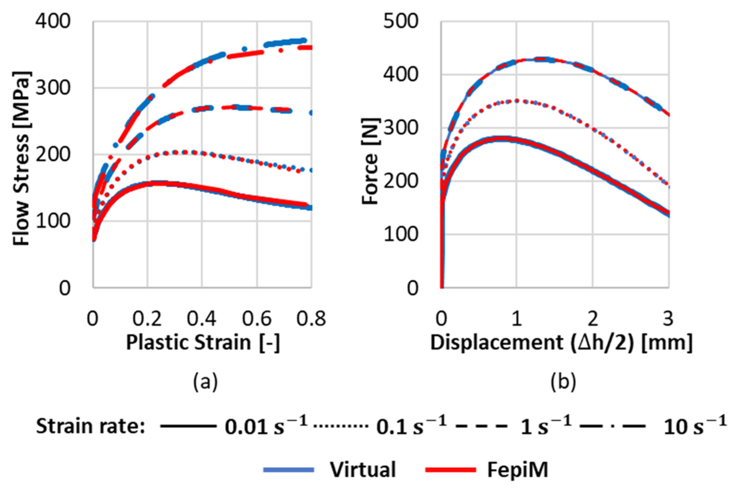
3.1. Results of FepiM Flow Curves Determined from Virtual Experiments

The goal of this section is to demonstrate the FepiM approach for tensile tests flow curves determination for the hot stamping steel 22MnB5. Therefore, the analytical flow curves for the same material are derived from the literature for the validation of the parallel optimization approach with virtual experiments. The hot compression test flow curves of 22MnB5 determined by Xu et al. [19] until a strain of 0.8 is considered by the author. Since the specimen used in this work exhibits necking in the plastic strain range of 0.25–0.30 for this material, the flow curves by Xu et al. are thought to be an appropriate choice to simulate necking and validate the parallel optimization approach. The flow curves obtained from [19] at 700 °C and strain rates of 0.01, 0.1, 1, and 10 s⁻¹ are shown as blue lines in Figure 5a.

The same FE model shown in Figure 1a is used for the virtual experiments and the complete flow curve field at 700 °C, shown as blue lines in Figure 5a, are given as an input to the model. The FE model consists of a total of 4314 C3D8 elements, where the smaller element size of 0.05 mm is considered in the deformation zone and the element size increases up to 0.2 mm at the end of the specimen, where the displacement is applied. The thickness of the specimen is represented by six elements. Three simulations are performed at nominal strain rates, namely 0.01, 0.1, and 1 s⁻¹. Here, nominal strain rates correspond to the displacement of the tool such that the strain rate in the gauge section remains constant (until necking begins). As discussed earlier, this strain rate can only be controlled and held constant until necking begins. Also, the flow curve at 10 s⁻¹ used in the simulation model is necessary to interpolate the flow curve data for the strain rate increase during necking for the virtual experiment at 1 s⁻¹. The output virtual FD curves from the three simulation models are shown in blue lines in Figure 5b. These virtual FD curves will now serve as an input to the parallel flow curve determination using FepiM.

Using the obtained virtual FD curves, the constant strain rate flow curves at 0.01, 0.1, and 1 s⁻¹ are determined in a parallel approach, as discussed in Section 2.1. Because flow curves at only one temperature were provided as input to the virtual experiments, isothermal conditions are assumed as a simplification for inverse flow curve determination as well. The results of the FepiM flow curves (red) in comparison with the flow curves provided as input to the virtual experiments (blue) are shown in Figure 5a. Apart from these three flow curves that are output from the inverse modeling, the flow curves at 10 s⁻¹ are also compared. This curve is obtained by the extrapolation of lower strain rate flow curves during the parallel flow curve determination approach and assists the flow curve assignment in UHARD during necking (using Equations (1) and (2)).

As seen by the red curves in Figure 5a, the FepiM approach could replicate the hardening behavior and predict the complex flow curve shapes at different strain rates. However, the FepiM flow curve at 10 s⁻¹ is slightly underestimating the analytical flow curves after a plastic strain of 0.4. The deviations could be attributed to the fact that this curve was obtained solely through logarithmic extrapolation and not from the FD curves provided as input to FepiM.

3.2. Discussion of FepiM Flow Curves Determined from Virtual Experiments

To quantitatively validate these results, the FepiM flow curves were again used in FE simulations of the tensile tests, and the FD curves from the simulations corresponding to each testing condition were extracted. The blue curves in Figure 5b depict a comparison of the FepiM FD curves and the virtual FD curves. The absolute relative error between the FD curves is obtained at every 0.05 mm displacement step, and the maximum error in the FepiM curves is 0.53% and corresponds to the simulation at 0.01 s⁻¹. Also, the average relative error ranges between 0.1 and 0.14%. The flow curve determined using the FepiM parallel approach could thus accurately replicate the virtual experiments. More importantly, the flow curves could replicate the FD curves of the virtual experiments even beyond the maximum force (after necking begins).

4. Conclusions

For tensile test specimens, especially under hot forming conditions, analytical methods based on correction factors have limited accuracy. Furthermore, these methods necessitate continuous measurement of necking throughout the experiment. However, equation-based methods have limited accuracy in representing complex flow curve shapes, and selecting an equation a priori is challenging. Since in tensile tests the strain rate cannot be maintained constant during deformation, the FepiM method is adopted in this report, where flow curves at different strain rates in the experimental matrix are determined in parallel. Interpolating between different flow curves that are determined in parallel allows for flow stress assignment in the necking zone. Also, an additional flow curve at a higher strain rate is approximated by extrapolation in order to assign the flow stress for the experiment at the highest strain rate in the experimental matrix.

This new approach is validated in this paper using virtual experiments, in which FD curves generated from simulations with known flow curve data are fed into FepiM. The output FepiM flow curves were able to accurately reproduce the flow curves used in the virtual experiments, with an average relative error of 0.1–0.14%. This procedure will be extended further to real experimental data in the future for the same material for flow curve determination at elevated temperatures.

References

1. Kopp, R.; Wiegels, H. Einführung in die Umformtechnik; Verlag Mainz: Aachen, Germany, 2023; ISBN 3-86073-821-6. [Google Scholar]
2. Sarafraz, Y.; Koch, A.; Felinks, N.; Biermann, D.; Walther, F. Influence of pre-drilling on hardness and tensile failure of formed internal threads in thin-walled AZ91 cast alloys. Eng. Fail. Anal. 2021, 130, 105783. [Google Scholar] [CrossRef]
3. Tu, S.; Ren, X.; He, J.; Zhang, Z. Stress–strain curves of metallic materials and post-necking strain hardening characterization: A review. Fatigue Fract. Eng. Mater. Struct. 2020, 43, 3–19. [Google Scholar] [CrossRef]
4. Hollomon, J.H. Tensile Deformation. Trans. Metall. Soc. AIME 1945, 162, 268–290. [Google Scholar]
5. Ramberg, W.; Osgood, W.R. Description of Stress-Strain Curves by Three Parameters; National Advisory Committee for Aeronautics: Hampton, VA, USA, 1943.
6. Yin, Q. Verfestigungs-und Schâdigungsverhalten von Blechwerkstoffen im Ebenen Torsionsversuch. Ph.D. Thesis, Dortmund Technische Universität, Dortmund, Germany, 2014. [Google Scholar]
7. Mecking, H.; Kocks, U.F. Kinetics of flow and strain-hardening. Acta Metall. 1981, 29, 1865–1875. [Google Scholar] [CrossRef]
8. Kocks, U.F.; Mecking, H. Physics and phenomenology of strain hardening: The FCC case. Prog. Mater. Sci. 2003, 48, 171–273. [Google Scholar] [CrossRef]
9. Roters, F.; Raabe, D.; Gottstein, G. Work hardening in heterogeneous alloys—A microstructural approach based on three internal state variables. Acta Mater. 2000, 48, 4181–4189. [Google Scholar] [CrossRef]
10. Xiong, W. Adoption of New Strategies for Parameterization of a Microstructure-Based Flow Stress Model. Ph.D. Thesis, Rheinisch-Westfälische Technische Hochschule Aachen, Aachen, Germany, 2017. [Google Scholar]
11. Bridgman, P.W. Studies in Large Plastic Flow and Fracture; Harvard University Press: Cambridge, MA, USA, 1952. [Google Scholar]
12. Gromada, M.; Mishuris, G.; Öchsner, A. Correction Formulae for the Stress Distribution in Round Tensile Specimens at Neck Presence; Springer: Berlin/Heidelberg, Germany, 2011; ISBN 978-3-642-22133-0. [Google Scholar]
13. Khoddam, S.; Solhjoo, S.; Hodgson, P.D. State of the art methods to post-process mechanical test data to characterize the hot deformation behavior of metals. Adv. Mech. Eng. 2021, 13, 168781402110610. [Google Scholar] [CrossRef]
14. Zhang, C.; Chu, X.; Guines, D.; Leotoing, L.; Ding, J.; Zhao, G. Dedicated linear—Voce model and its application in investigating temperature and strain rate effects on sheet formability of aluminum alloys. Mater. Des. 2015, 67, 522–530. [Google Scholar] [CrossRef]
15. Kamaya, M.; Kitsunai, Y.; Koshiishi, M. True stress–strain curve acquisition for irradiated stainless steel including the range exceeding necking strain. J. Nucl. Mater. 2015, 465, 316–325. [Google Scholar] [CrossRef]
16. Vuppala, A.; Krämer, A.; Braun, A.; Lohmar, J.; Hirt, G. A New Inverse Explicit Flow Curve Determination Method for Compression Tests. Procedia Manuf. 2020, 47, 824–830. [Google Scholar] [CrossRef]
17. Vuppala, A.; Krämer, A.; Lohmar, J.; Hirt, G.; Fepi, M. A Novel Inverse Piecewise Method to Determine Isothermal Flow Curves for Hot Working. Metals 2021, 11, 602. [Google Scholar] [CrossRef]
18. Vuppala, A.; Brüggemann, H.; Bailly, D.; Scharifi, E. An Inverse Piecewise Flow Curve Determination Method for Torsion Tests at Elevated Temperature. Metals 2025, 15, 219. [Google Scholar] [CrossRef]
19. Xu, Y.; Birnbaum, P.; Pilz, S.; Zhuang, X.; Zhao, Z.; Kräusel, V. Investigation of constitutive relationship and dynamic recrystallization behavior of 22MnB5 during hot deformation. Results Phys. 2019, 14, 102426. [Google Scholar] [CrossRef]
Figure 1. (a) FE model of the tensile test specimen at the gauge section, (b) inputs and a stepwise approach for FepiM flow curve determination for tensile tests.
Metals 15 00638 g001
Figure 2. Flow chart illustrating parallel FepiM optimization for tensile tests.
Metals 15 00638 g002
Figure 3. Illustration of interpolation in UHARD during necking.
Metals 15 00638 g003
Figure 4. Illustration of the FD curves used for virtual experiments.
Metals 15 00638 g004
Figure 5. (a) Comparison of flow curves used in virtual experiments with the FepiM flow curves, (b) comparison of FD from virtual experiments with the FepiM flow curves.
Metals 15 00638 g005
Disclaimer/Publisher’s Note: The statements, opinions and data contained in all publications are solely those of the individual author(s) and contributor(s) and not of MDPI and/or the editor(s). MDPI and/or the editor(s) disclaim responsibility for any injury to people or property resulting from any ideas, methods, instructions or products referred to in the content.