Prediction of Medium-Thick Plates Weld Penetration States in Cold Metal Transfer Plus Pulse Welding Based on Deep Learning Model

Abstract

During the cold metal transfer plus pulse (CMT+P) welding process of medium-thick plates, problems such as incomplete penetration (IP) and burn-through (BT) are prone to occur, and weld pool morphology is important information reflecting the penetration states. In order to acquire high-quality weld pool images under complex welding conditions, such as smoke and arc light, a welding monitoring system was designed. For the purpose of predicting weld penetration states, the improved Inception-ResNet prediction model was proposed. Squeeze-and-Excitation (SE) block was added after each Inception-ResNet block to further extract key feature information from weld pool images, increasing the weight of key features beneficial for predicting the penetration states. The model has been trained, validated, and tested. The results demonstrate that the improved model has an accuracy of over 96% in predicting penetration states of aluminum alloy medium-thick plates compared to the original model. The model was applied in welding experiments and achieved an accurate prediction.

1. Introduction

Medium-thick plates (4.5~25 mm) are mainly used in mechanical manufacturing, container manufacturing, communications, the transportation industry, and other fields, including storage and transportation tanks in the energy and chemical industry, etc. [1]. Cold metal transfer (CMT) welding is widely used due to its advantages of not producing slag splashing and low heat input, alternating cold and hot cycles, almost zero current during droplet transition, and faster welding speed [2]. 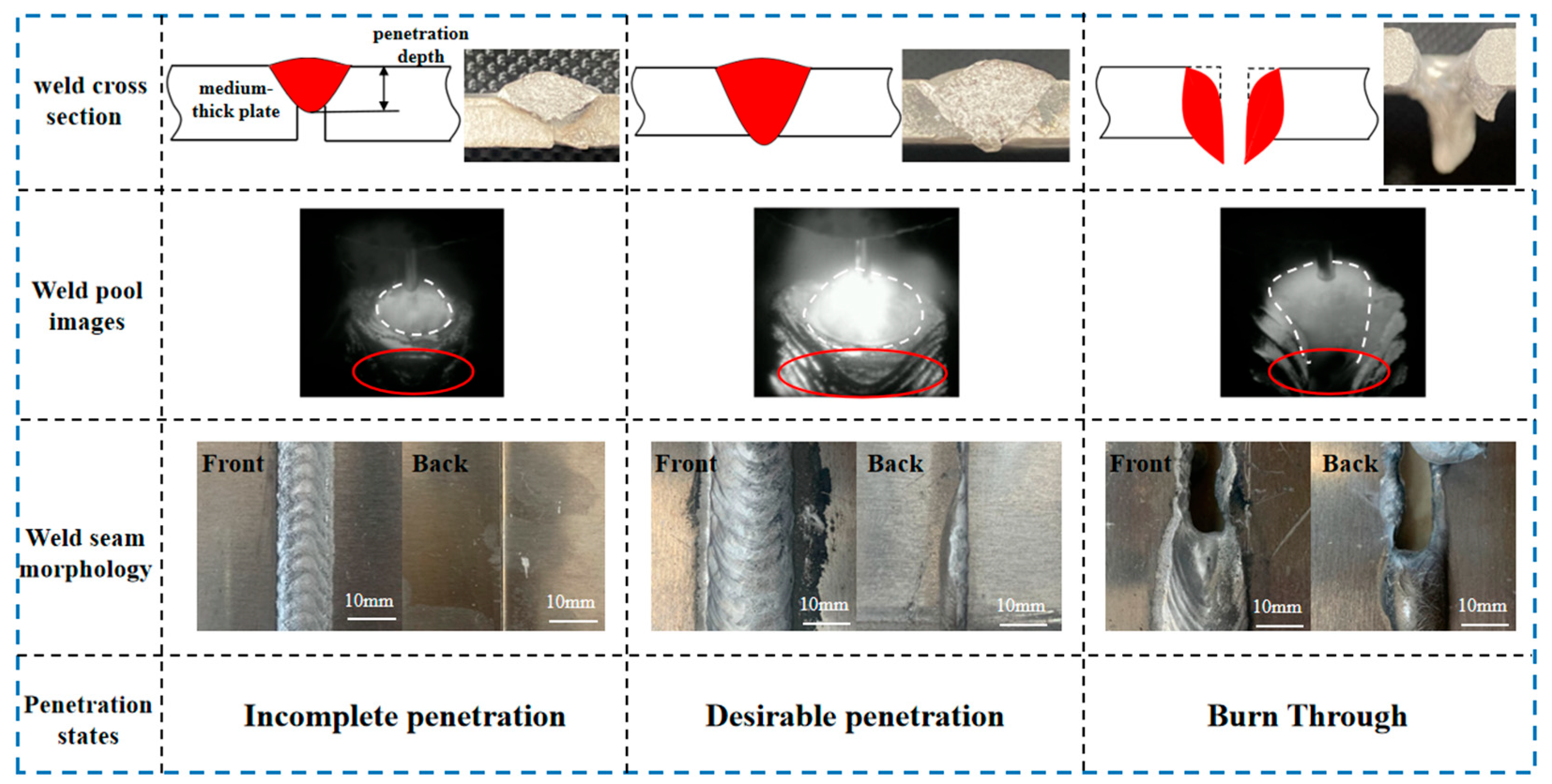However, pure CMT welding cannot achieve the welding of medium-thick plates, so the cold metal transfer plus pulse (CMT+P) welding process was proposed [3]. Within this mode, the short-circuit transition from CMT mode and single droplet transmission from pulse mode are combined. The deposition rate is increased during operation by alternating between the pulse mode and the CMT mode, adding a droplet in each cycle. Medium-thick plate welding is sensitive to process variables, and there is a limited range of acceptable settings. The welding quality of medium-thick plates is impacted by welding flaws, including incomplete penetration (IP) and burn-through (BT), which are particularly common in lengthy welding seam welding operations. Traditional testing methods like appearance inspection, X-ray non-destructive testing, ultrasonic testing, and others are unable to detect welding defects like IP and BT in real time while welding is taking place. Instead, they can only do so after welding is finished, which surely results in material waste [4]. The quality of the weld formation may be reflected by some information about the welding process, including light and sound signals, variations in welding voltage and current, and the morphology and temperature of the weld pool throughout the welding process. Therefore, how to realize high-quality monitoring-related information on the welding process and accurately predict the weld penetration states based on key information acquired during the welding process, such as welding sound, weld pool images, etc., has gradually become a research hotspot [5,6].

Machine vision is gradually gaining popularity in the field of welding manufacturing due to its advantages of safety, reliability, low cost, and real-time performance [7]. Real-time welding process monitoring is achieved by selecting different industrial cameras to monitor the weld pool throughout the welding process based on varied work circumstances [8]. The two categories of machine vision methods are active and passive vision. Active vision works on the basis of external light sources [9]. Gao et al. [10] designed an active vision system using the characteristics of the weld pool contour in the laser welding process by illuminating the weld pool with a laser and generating a contour shadow section; the camera receives light radiation from the laser and quantitatively describes the relationship between the weld pool morphology and the stability of the welding process by analyzing the weld pool contour parameters. Cheng et al. [11] used a camera to capture images of the weld pool reflected from a single-stripe laser generator and investigated the key differences between partially and fully penetrated camera-received images. The passive vision method does not require any additional light source equipment and directly uses a welding light source or natural light source as background light sources when capturing images with industrial cameras. Compared to active vision, the equipment cost is lower. Chen et al. [12] designed a passive vision image acquisition system by placing a bandpass filter in the near-infrared band in front of the camera lens to reduce the interference of arc light, information on the weld pool width, tail length, and surface height that eliminates some arc light can be obtained. Liang et al. [13] designed a biprism stereovision passive vision system to sense the weld pool surface under different penetration states during pulsed gas metal arc welding (GMAW-P) with a V-groove joint.

Weld penetration states are crucial information for the quality of the weld formation, and the morphology of the weld pool is an important factor reflecting the weld penetration states [14,15,16,17,18]. Monitoring weld pool morphology based on machine vision during the welding process, predicting weld penetration states accurately, and adaptively adjusting welding parameters are key technologies for intelligent welding [19,20]. The penetration states recognition development of the welding process based on the weld pool morphology is considerably improved by deep learning (DL) and image processing technology (IPT) in the area of intelligent welding [21,22]. Convolutional neural networks (CNNs) are an important component of deep learning due to their outstanding performance in image recognition and prediction in recent years, which have gradually become widely used in the field of welding process monitoring [23]. Currently, there are two primary ways that are used to gather information representing penetration states based on machine vision: dynamic continuous weld pool images and single weld pool images. As for dynamic continuous weld pool images, scholars commonly combined CNN models with long-short-term memory (LSTM) networks to study the time series dependency features of dynamic continuous weld pool images that represent the penetration states. Yu et al. [24] developed a CNN-LSTM model to extract features from dynamic continuous time series weld pool images, aiming to achieve an accurate prediction of weld back width. Zhou et al. [25] proposed a novel model based on the CNN-LSTM model to extract both the spatial and temporal features of weld pool images, and in key welding scenarios, predicted values close to the actual penetration status were obtained, and more than 80% accuracy was achieved in predicting the next 2 s of keyhole behavior. However, a significant number of datasets are required to train the model because of the excessive parameters of CNN-LSTM. In the case of limited weld pool datasets, the CNN-LSTM model has poor performance in characterizing weld pool features, thereby reducing the accuracy of model predictions.

Under different penetration states, the situation of the weld pool and its surroundings will vary greatly. A single weld pool image has sufficient information to reflect the welding quality, including the size of the weld pool contour, the shape of the weld seam, etc. In recent years, with the rapid development of CNN, their accuracy and speed in image recognition and prediction have been greatly improved. The current mainstream CNN models include LeNet [26], AlexNet [27], VGGNet [28], GoogLeNet (Inception) [29], and ResNet [30], etc. Inception and ResNet are two typical network structures of CNNs, which are the most representative in the development process. The method to improve the performance of neural networks is generally to increase the depth and width of the network, where depth refers to the number of network layers and width refers to the number of neurons. The inception network is different from previous networks in that it no longer aims to increase the number of vertical network layers to improve model performance. Instead, it designs a sparse network structure that can generate dense data, not only increasing the width of the network and improving neural network performance but also increasing the adaptability of the network to scale, ensuring the efficiency of computing resource utilization. ResNet has made significant innovations in network structure rather than simply stacking layers. By using residual connections, the original features can be preserved, making the learning of the network smoother and more stable, further improving the accuracy and generalization ability of the model, and solving problems such as vanishing, exploding, and degenerating gradients caused by excessive network layers. A lot of welding monitoring research is based on these two networks. Li et al. [31] proposed a Residual-Group convolution model (Res-GCM) based on the ResNet block to predict the penetration states by feature extraction and analysis of welding images in non-penetrating laser welding, which achieved an accuracy of 90.53%. Feng et al. [32] designed a DeepWelding framework, which integrates image preprocessing, image selection, and weld penetration classification. Among them, based on five classic convolutional neural network weld penetration modules, ResNet achieved the highest accuracy of 78.9%, 99.5%, and 88.1% in the three datasets, respectively. Wang et al. [33] proposed a semantic segmentation network, Res-Seg, based on the ResNet-50 network to extract the contour of the molten pool in TIG stainless steel welding, which achieved an accuracy of 92.14%. Sekhar et al. [34] studied the classification of tungsten inert gas (TIG) welding defects using eight pre-trained typical convolutional neural networks combined with four optimizers. The accuracy rates of Inception were 92.15%, 85.83%, 91.68%, and 86.81%, respectively. Oh et al. [35] proposed a Faster R-CNN for automatically detecting welding defects, comparing two internal feature extractors (ResNet and Inception-ResNet) of Faster R-CNN and evaluating their performance.

As described above, Inception and ResNet networks are widely used in the classification of welding defects and prediction of weld penetration states, but few of them consider combining the advantages of Inception and ResNet networks. The DL model needs to accurately predict the penetration states. Only in this way can it serve as a basis for adjusting more reliable welding process parameters during the welding process. In the process of monitoring the penetration states of medium-thick plate welding, the changes in weld pool morphology between IP, desirable penetration (DP), and BT are difficult to distinguish, especially in complex and harsh welding environments. Therefore, it is difficult to accurately recognize and predict the penetration states of medium-thick plate welding.

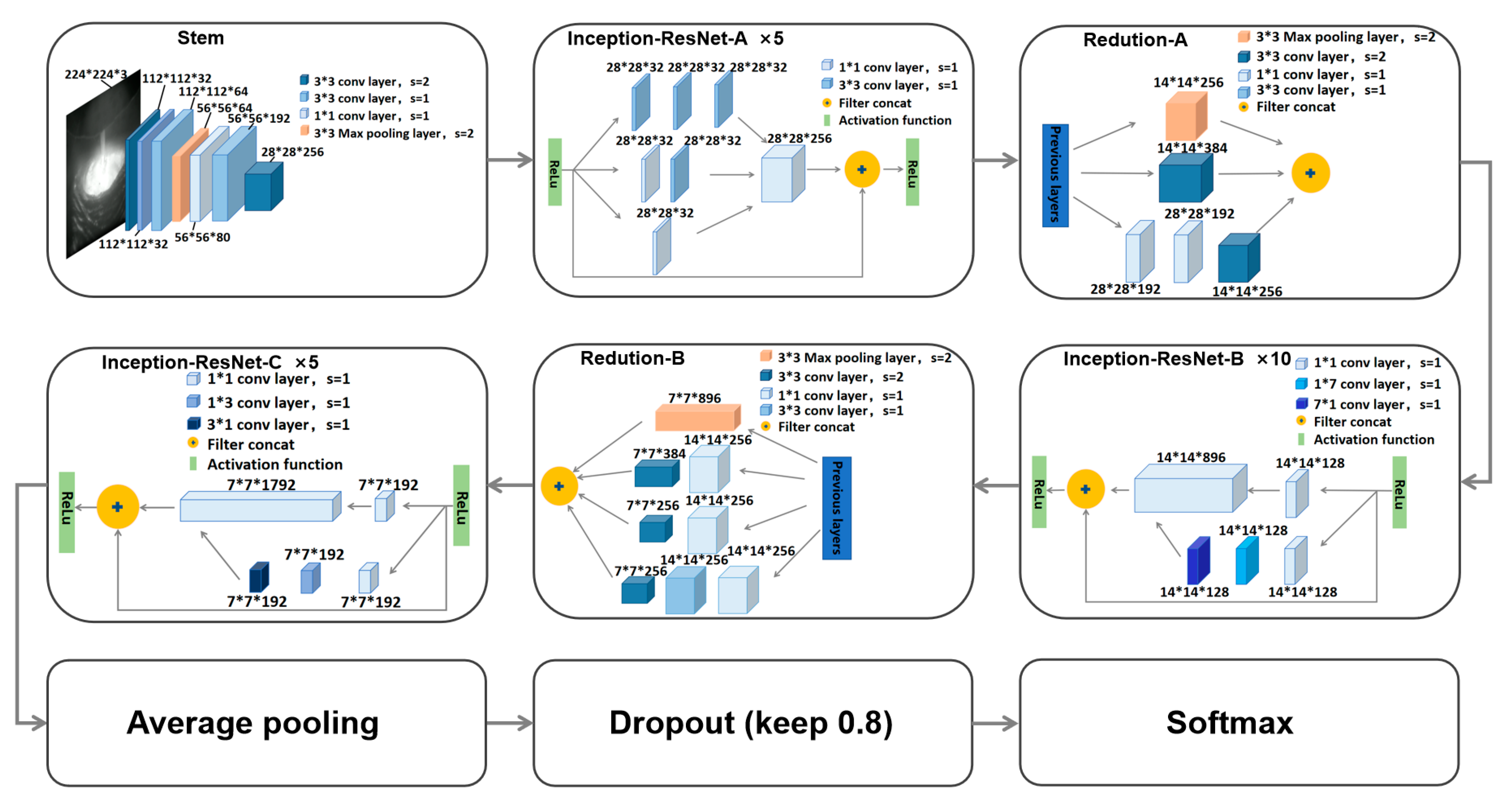
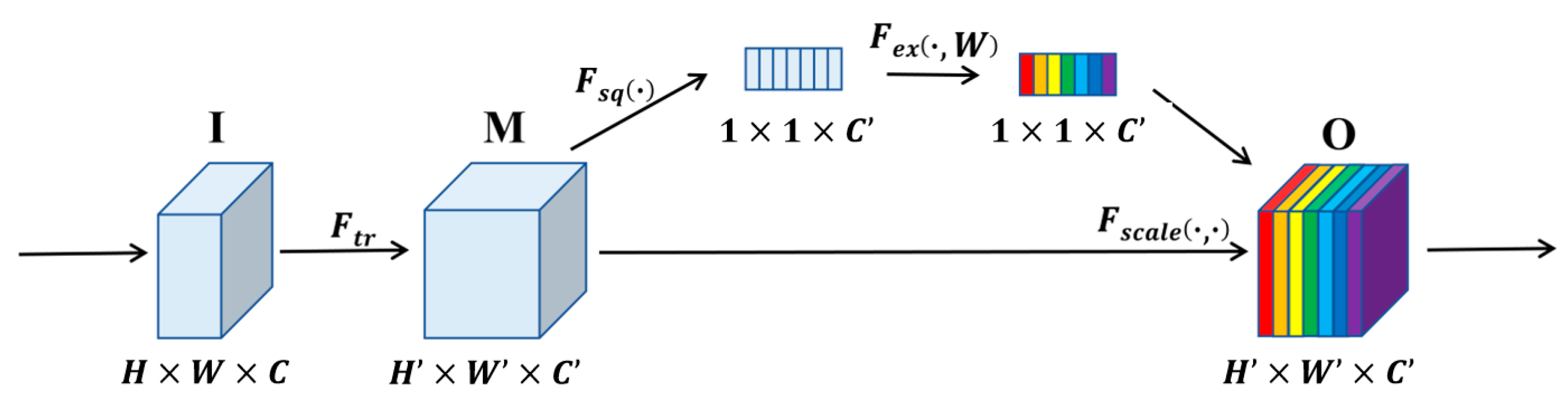
To solve the issues of difficulty in distinguishing the morphology of the weld pool in the welding process of medium-thick plates and accurately predicting the penetration states, a method for predicting the weld penetration states of medium-thick plates welding in complex interference sources was proposed based on a DL model. To achieve clear monitoring of weld pool morphology in complex welding environments, such as smoke and strong arc light, a welding monitoring system was designed. Based on this system, welding experiments of aluminum alloy medium-thick plates were carried out under different process parameters, and high-quality weld pool image datasets were obtained. A weld penetration states prediction model based on improved Inception-ResNet has been established, which adds an SE block after each Inception-ResNet block, recalibrating the weights of key features of the weld pool, enhancing the model’s ability to better extract key feature information, and significantly improving model performance in predicting penetration states. The model is trained, validated, tested, and finally embedded into the weld pool monitoring platform and applied to the actual welding experiments.

2. Experimental Method

2.1. System Configuration

The overall system configuration is shown in Figure 1. The welding experimental system mainly consists of a welding robot (KR6-C, KUKA, Augsburg, Germany), 99.99% pure argon, an elevated control cabinet (KRC4, KUKA, Augsburg, Germany), a welding power supply (TPS5000, Fronius, Pettenbach, Austria), a teach pendant (SmartPAD, KUKA, Augsburg, Germany), and a welding monitoring system (Xiris, Burlington, ON, Canada).

The welding monitoring system mainly consists of a monocular industrial charge-coupled device (CCD) camera (XVC-1000, Xiris, Burlington, ON, Canada), a “7”-shaped fixture, an image workstation, a narrow band filter with a wavelength of 670 mm, and a 10% light transmittance attenuator.

Table 1. Camera parameters.

Camera Parameters	Value
Camera model	XVC-1000
Sensor	Color HDR
Resolution ratio	1280 (H) × 1024 (V)
Pixel size (μm)	6.8 × 6.8
Pixel bit depth (bits)	12
Frame rate (fps)	55

displays the specifications of the camera. The camera is mounted in a welded robotic arm through the “7”-shaped fixture, and the filter and attenuator are installed on the camera. After multiple welding tests and installation position adjustments, the best-quality images of the entire weld pool were acquired. The ideal position is to install the camera at the rear of the welding torch and set it up at a 30° tilt angle, with the camera lens 117 mm from the torch mouth, making it easy to obtain a high-quality weld pool image during the welding process. The narrow band filter with a wavelength of 670 mm was chosen after taking into account the intensity range of each wavelength, and it successfully suppressed powerful arc light in welding applications. Nevertheless, the surrounding area of the weld pool is too bright to see the contour of the weld pool during the pulse peak stage. After installing the 10% light transmittance attenuator, the camera effectively reduces stronger arc interference during the peak pulse stage and obtains clear contour images of the weld pool during this stage. On the image workstation, the acquired images were processed. The camera follows the welding torch as it acquires the weld pool images, which are then sent to the image workstation for further processing. XirisWeldStudio software version 2.0.4 and a Gigabit Ethernet link were then used to transport the digital images to a high-performance graphics workstation. This procedure produced training, validation, and testing datasets for the prediction model that was used later.

2.2. Welding Experiments

The welding experiments of aluminum alloy medium-thick plates were conducted to verify the performance of the model. The welding experiments were conducted with base material of 5083 aluminum alloy (Alcoa Corporation, Pittsburgh, PA, USA), and the specimen’s size was 150 mm × 100 mm × 6 mm, as shown in Figure 2. The welding wire of AlMg4.5MnZr with a diameter of 1.2 mm was selected. The main components of 5083 aluminum alloy and AlMg4.5MnZr welding wire are shown in

Table 2. Chemical composition of 5083 aluminum alloy (Wt%).

Composition	Si	Fe	Cu	Mn	Mg	Zn	Cr	Ti	Al
Wt.%	0.25	0.30	0.10	0.60	4.50	0.15	0.10	0.10	Bal.

and

Table 3. Chemical composition of AlMg4.5MnZr welding wire (Wt%).

Composition	Si	Fe	Cu	Mn	Mg	Zn	Cr	Ti	Al
Wt.%	0.25	0.40	0.05	1.00	5.20	0.25	0.25	0.15	Bal.

.

Table 4. Welding conditions applied for welding experiments.

Welding Conditions	Welding Parameters
Material	5083 aluminum alloy
Welding type	CMT+P
Welding speed	0.28–0.44 m/min
Wire feeding speed	8.0–9.6 m/min
Pulse frequency	2~3 Hz
Wire	AlMg4.5MnZr
Wire diameter	1.2 mm φ
Groove type	No groove
Shielding gas	99.9% Argon
Gas flow rate	18~20 L/min

displays the particular welding parameter settings. Weld pool characteristics in welding experiments are directly impacted by the welding settings that are specified. The welding parameters consist of wire feeding speed, ambient temperature, welding current, welding voltage, and shielding gas rate. The welding equipment utilized for this experiment has monolithic welding settings, meaning that changing one welding parameter would cause the other parameters to alter proportionately as well. Without activating the torch ignition mode, the wire feeding speed is progressively raised from 138 A to 180 A, changing the welding voltage and welding current. Figure 3 illustrates the connection between the welding process parameters. We are limited to concentrating on one of the three factors. In addition to the built-in parameters of the welding system, welding speed is also an important welding parameter. So this work primarily focuses on two important welding parameters: wire feeding speed and welding speed.

During the welding process, the medium-thick plates are fixed under the welding torch with a jig, and the welding torch moves along the weld seam. Then, 99.9% pure argon gas is blown as a protective gas around the weld pool during the welding process, avoiding metal oxidation during the welding process. The camera follows the welding torch to obtain weld pool images. Always maintain a constant distance between the camera and the weld seam during the welding process to ensure the validity of the obtained weld pool images. To get a huge number of images needed for the model’s subsequent training, the welding process parameters were set somewhat broader than the proper welding parameter range. The welding process parameters are shown in

Table 5. Welding conditions applied for experiments.

Number	Welding Speed (m/min)	Wire Feeding Speed (m/min)	Penetration States
1	0.28	8.0	IP
2	0.30	8.2	IP
3	0.32	8.4	DP
4	0.34	8.6	DP
5	0.36	8.8	DP
6	0.38	9.0	BT
7	0.40	9.2	BT
8	0.42	9.4	BT

, and a total of 8 welding experiments were set up, including 2 groups of IP experiments, 3 groups of DP experiments, and 3 groups of BT experiments. The welding parameters for each group, such as wire feeding speed and welding speed, are set according to the table data, and the welding process parameters for each group remain unchanged during the welding process. The pixel size of the obtained weld pool image is 1280 × 1024, and it is transmitted to the image workstation for image processing.

3. The Prediction Model of Penetration States

3.1. Principle of CNNs

CNNs are one of the popular directions developed with machine vision and artificial intelligence technologies and are widely used in image classification, natural language processing, and other fields [36]. CNNs consist of an input layer, convolutional layers, pooling layers, and a fully connected layer [37]. The convolutional layer consists of a number of convolutional kernels, and the convolutional computation is performed by traversing the previous input layer through the convolutional kernels, multiplying the corresponding elements, and summing them. The Equation (1) [38] is the eigenvalue $Z_{i,j,k}^l$ of the kth feature map location in layer l at:

$$Z_{i,j,k}^l={{\displaystyle W_k^l}}^T{x}_{i,j}^l+b_k^l$$

(1)

where $W_k^l$ and $b_k^l$ are the weight parameters and bias of the kth convolutional kernel in layer l. $x_{i,j}^l$ is the input feature map centered on the location in layer l.

Each convolutional kernel is shared when traversing the previous layer’s input, and this parameter sharing reduces model complexity and makes the network easier to train. The activation function is required for multilayer neural networks to detect nonlinear features. Typical activation functions are sigmoid [39], tanh [40], and ReLu [41]. The activation function is shown in Equation (2), as follows:

$$a_{i,j,k}^l=\sigma (Z_{i,j,k}^l)$$

(2)

where $\sigma (·)$ denotes the activation function, $a_{i,j,k}^l$ denotes the activation value, and $Z_{i,j,k}^l$ denotes the feature value.

The pooling layers reduce the feature map size and ensure that the features are translation invariant. Typical pooling operations are average pooling (Ave-pooling) and maximum pooling (Max-pooling). Let the pooling function be pool (∙), for each activation value, with the Equation (3):

$$y_{i,j,k}^l=pool(a_{m.n.k}^l),\forall (m,n)\in R_{i,j}$$

(3)

where $R_{i,j}$ is the local neighborhood around location $(i,j)$.

The size of the new feature map output after the series of operations in CNN is determined by the convolution kernel size, pooling layer size, padding size, and stride size, as shown in Equation (4):

$$Output size={\displaystyle \frac{W+2P-F}{S}}+1$$

(4)

where $W$ is input size, $P$ is padding size, $F$ is the size of the filter, includes convolution and pooling operation, and $S$ is stride size.

After some convolutional and pooling layers, there will be one or even more fully connected layers, with the aim of integrating and then normalizing features that have been highly abstracted after several convolutions, with $N$ sample sizes, $n$∈ (1, …, $N$), and the loss L can be defined as Equation (5):

$$L={\displaystyle \frac{1}{N}}{\sum }_{n=1}^{N}l(\theta ;y^{(n)},o^{(n)})$$

(5)

where $y^{(n)}$ is the true value, $o^{(n)}$ is the predicted value, and $\theta$ are the parameters in the CNN (weights, bias, etc.). By minimizing the loss, the best weights for the model can be obtained.

3.2. Data Preparation

The various penetration states illustration are shown in Figure 4. The obtained weld pool images contain sufficient information to reflect the penetration states of the weld seam. The shapes of the weld pools in the three penetration states are shown by the white dotted lines in Figure 4, and the weld textures at the tail of the weld pool are indicated by the red solid lines. When welding with IP process parameters, the image obtained has a smaller weld pool area and a shape similar to a circle. Due to the smaller top weld pool area, the energy required for melting the base metal downwards along the thickness direction is insufficient, resulting in IP. At the same time, other areas outside the weld pool, such as the base metal substrate, are all black, with a larger area and unclear weld texture; When welding with DP process parameters, the area of the weld pool in the image obtained is significantly larger than that in the case of IP. Although the shape of the weld pool is also similar to a circular shape, the larger weld pool area reflects that there is more molten metal. When melting the base metal downwards along the thickness direction, the energy is sufficient to achieve DP, and the weld texture is clear. The area of the base metal substrate outside the weld pool is also smaller, which is significantly different from the image obtained in the case of IP; the shape of the weld pool obtained during welding using the BT process parameters is similar to an ellipse, and the area becomes smaller. This is because a large amount of molten metal flows out of the base material along the thickness direction along the welding gap, while there is less remaining molten metal at the top. At the same time, the texture at the weld seam is not clear, especially when the tail of the weld seam appears black, indicating that the base material has been burned through.

From the principle of welding experiments and the appearance of welded joints after welding. IP is caused by low heat input energy, which prevents the molten metal weld pool from melting all of the plates in the direction of plate thickness. As a consequence, the penetration depth is less than the plate thickness. The primary feature of the plate after welding is that the front side has been welded and the back side has not. DP occurs when the heat input energy is appropriate and the penetration depth of the metal weld pool is equal to or slightly more than the plate thickness. The main characteristic of the plate after welding is the formation of robust welds on both the front and back surfaces. BT is caused by an excessive amount of heat input energy and the initial size of the weld pool will also be slightly larger compared to other penetration states. However, as the heat input energy accumulates, it causes the molten metal to flow and drip into the gaps instead of forming a weld seam. The primary feature is that after welding, the space between the plates widens as the molten metal in the weld pool flows downward.

It is necessary to construct the weld pool image dataset before building the DL model. The weld pool images were originally taken by the camera at 1280 × 1024 pixels; they were resized to 224 × 224 pixels in order to be used as model inputs. Weld pool images and matching penetration labels should be included in every dataset. The weld pool images were categorized into three groups: IP, DP, and BT, with labels set to 0, 1, and 2, respectively. The weld pool images and labels for each of the three kinds of penetration states are shown in Figure 5. It is evident from the image that the weld pool under IP conditions is smaller, which is in line with the real circumstances. When IP circumstances apply, the weld pool is smaller than when DP conditions apply. The weld pool under BT conditions is different from the other two types, and the weld pool becomes slender and has a tendency to flow. The number of images corresponding to each category is shown in

Table 6. The number of images corresponding to each category and the data partitioning for the model.

Label	Penetration State	Training Data	Validation Data	Testing Data	Total Number of Image Data
0	IP	2800	718	400	3918
1	DP	1050	270	252	1572
2	BT	1960	502	350	2812

, and image data partitioning for model training, validation, and testing. We obtained different weld pool image data from each group of welding experiments. According to the weld pool characteristics under the corresponding welding parameters of each group, a total of 8302 frontal weld pool images were selected, and 5810 of them were randomly extracted as training data, 1490 as validation data, and 1002 as testing data.

3.3. Structure of the Inception-ResNet and Improved Model

Combining the structural properties of Inception’s ability to build deep models with the advantages of the ResNet residual module, the improved Inception-ResNet model was proposed for weld penetration states prediction. The structure of the Inception-ResNet model is shown in Figure 6.

The model includes the Stem block, the Inception-ResNet-A block, the Inception-ResNet-B block, the Inception-ResNet-C block, and the Redution-A and Redution-B blocks [42]. The network has a deeper structure thanks to the Stem block. The Inception-ResNet block combines the benefits of the Inception and ResNet blocks, maintaining the network’s sparsity features while also greatly accelerating network training. The Redution block was used to change the width and height of the neural network. The detailed structure of the Inception-ResNet model is shown in Figure 7.

Based on the original model, the structure of Inception-ResNet was optimized; the specific improved model is shown in Figure 8. In each loop, the Squeeze-and-Excitation (SE) block was added, which will reweight each channel, allowing different channels to have different effects on the weld pool key features. The block increases the proportion of weld pool key feature information in the multi-layer network, which does not change the feature map’s dimensions. The normalization is set to 3, considering that the weld pool has three types of penetration states. The SE block is shown in Figure 9.

$F_{tr}$ is one or a set of convolution operations: $I\to M,I\in H\times W\times C,M\in H^{\prime }\times W^{\prime }\times C^{\prime }$. The feature map $M$ that has undergone a convolution operation first goes through the ‘Squeeze’ operation ($F_{sq}$), which cross-spatial dimension $H^{\prime }\times W^{\prime }$ feature map to generate channel descriptor: $1\times 1\times W^{\prime }$. After that, an ‘excitation’ operation ($F_{ex}$) will be done, by using specific excitation mechanisms to reweight different channels, increasing the weight of weld pool key features, and then sending the changed feature map $O$ as the output of the SE block to subsequent layers [43]. SE block further extracts features from the feature map outputted by Inception-Resnet. Firstly, the input feature map is squeezed into one-dimensional data through global average pooling, reducing the dependency between different channels, and obtaining a global receptive field of $H\times C$, with a wider receptive area. Then, the degree of importance of the weld pool feature information contained in each channel is obtained through fully connected layers, and different weight parameters are reassigned. Finally, the weight values of each channel calculated by the SE block are multiplied by the two-dimensional matrix of the corresponding channel in the original feature map to obtain a new feature map with reweighted parameters. SE block increases the weight of weld pool key feature information that reflects the penetration states in the feature map and reduces the weight of useless feature information to achieve recalibration of weight parameters in the original feature map, thereby increasing sensitivity to key weld pool feature information. At the same time, this block is lightweight and flexible to use, which can be easily applied in networks and significantly improve the performance of the model.

4. Results and Discussion

4.1. Model Performance and Comparison

All training, validation, and testing of the model were conducted on a DELL T7920 PC (DELL, Round Rock, TX, USA) coupled with an RTX3060Ti graphics card (NVIDIA, San Jose, CA, USA). To train the model, it was required to set parameters like learning rate, number of iterations, and convolution kernel size, taking into account factors like data fitting and convergence, saving computing time, etc. Moreover, the gradient descent method was used for training, and weights were updated in a timely manner. The learning rate might be first set quite high and then changed once again in the following process. The testing dataset would use the weight that showed the highest performance on the validation dataset.

Table 7. Training parameters of the model.

Training Parameters	Parameter Value
Img_size	224 × 224 × 3
Batch_size	32
Learning_rate	0.001
Weight_variable	0.005
Max_iter	5000
Solv_mode	CPU
Numbers of epochs	10
Loss function	Cross_entropy

displays the settings for the model. Currently, the loss functions mainly include regression loss functions (mean square error (MSE) loss function and mean absolute error (MAE) loss function) and classification loss functions (cross-entropy loss function). Among them, the cross-entropy function is often used to solve classification problems, including binary classification problems and multi-classification problems. The binary classification cross-entropy loss function is as shown in Equation (6):

$$L={\displaystyle \frac{1}{N}}{\sum }_{n=1}^N-(y^{(n)}\log (p^{(n)})+(1-y^{(n)})\log (1-p^{(n)}))$$

(6)

where y⁽ⁿ⁾ represents the label of sample n. The positive class is 1 and the negative class is 0; p⁽ⁿ⁾ represents the probability that the sample, and n is predicted as the positive class. For multi-classification problems, the cross-entropy loss function is as shown in Equation (7):

$$L=-{\displaystyle \frac{1}{N}}{\sum }_{n=1}^N{\sum }_{c=0}^M{y}^{(nc)}\log (p^{(nc)})$$

(7)

where M represents the number of classification categories, y^(nc) represents the sign function (0 or 1), and p^(nc) represents the probability that the sample n belongs to category c.

Three penetration states of IP, DP, and BT are included in the output results of the weld pool penetration states prediction in this study. As a result, the model was trained using weld pool images with three groups, and the step size determined the quantitative output of the loss function value. Each prediction result has a loss value change curve; the faster the curve converges and the lower the numerical value, the better the model performance. At the same time, outputting a loss value for every 10 training sessions. The results of the model training process are shown in Figure 10. The original model and the improved model with the SE block were trained independently. The improved model has a greater Initial training accuracy and lower loss values than the original model, as can be seen in the figure. Following 2000 steps, the training of the models begins to settle, and both models reach 100% accuracy with loss values lowered to 0. Though this does not guarantee that the improved model will perform better overall, it does outperform the original model in the training dataset. In the validation and testing dataset, further testing is required.

Figure 11 displays both models’ performance in the validation dataset. The original model reached stability after a few epochs, and the final model’s accuracy stayed at about 90%. The improved model, however, continued to achieve an accuracy of almost 95% over many epochs, demonstrating that the SE block’s attention mechanism is capable of successfully extracting features for penetration recognition, hence raising the model’s penetration prediction accuracy.

4.2. Confusion Matrix

As seen in Figure 12, the results of the model’s prediction of test dataset images of various penetration states were converted into a confusion matrix in order to analyze the model’s accuracy in predicting distinct penetration states [44]. The indicators used to evaluate the performance of a model include accuracy, loss, confusion matrix, etc. The confusion matrix shows the true belonging category of the data in each row, the number of data instances in each row as the total number of data instances in that category, and the number of real data instances predicted to belong to that category as each column’s numerical values. The anticipated category is represented by each column, and the total number of each column indicates the anticipated quantity of data for that category.

There are four parameters in the confusion matrix that reflect the classification performance of the model: true positive ($TP$), true negative ($TN$), false positive ($FP$), and false negative ($FN$). Furthermore, the classification accuracy rate can be regarded as an indicator that measures the proportion of a given set of samples in the dataset being correctly classified into the actual target category. The specific calculation method is as shown in Equation (8):

$$Accuracy={\displaystyle \frac{TP+TN}{TP+TN+FP+FN}}$$

(8)

Accuracy is the most direct indicator for evaluating classification models, but its drawbacks are also obvious. When the proportions of different categories of samples are severely imbalanced, the category with the larger proportion will be the most significant factor affecting the accuracy rate. In addition, precision represents the proportion of actual positive samples among the samples whose predicted results are positive. The specific calculation method is as shown in Equation (9):

$$Precision={\displaystyle \frac{TP}{TP+FP}}$$

(9)

Recall represents the prediction result as the proportion of actual positive samples in the positive samples of the entire sample. The specific calculation method is as shown in Equation (10):

$$Recall={\displaystyle \frac{TP}{TP+FN}}$$

(10)

The F1 score is a weighted average of precision and recall. The specific calculation method is as shown in Equation (11):

$$F1 score={\displaystyle \frac{2(Precision\times Recall)}{Precision+Recall}}$$

(11)

Based on these indicators, the performance of the original model and the improved model in predicting different penetration states can be evaluated. The results are shown in

Table 8. The Accuracy, Precision, Recall, and F1 score of the original model.

Penetration States	Accuracy	Precision	Recall	F1 Score
IP	0.911	0.958	0.902	0.929
DP		0.811	0.905	0.855
BT		0.942	0.926	0.934

and

Table 9. The Accuracy, Precision, Recall, and F1 score of the improved model.

Penetration States	Accuracy	Precision	Recall	F1 Score
IP	0.967	0.975	0.962	0.968
DP		0.931	0.964	0.947
BT		0.986	0.974	0.980

.

By comparing the confusion matrices of the two models, the prediction accuracy of the improved model is significantly higher than that of the original model. The classification accuracy of the original model was 91.1%. As an indicator for measuring the comprehensive performance of the model, the F1 score of the DP classification was 0.859, which was significantly lower than that of other classifications. The performance of the improved model was overall superior to that of the original model. The accuracy was 96.7%. The precision and recall rates of BT classification were the highest, reaching 98.6% and 97.4%, respectively. As an indicator for measuring the comprehensive performance of the model, the F1 scores of the three classifications (IP, DP, and BT) were significantly higher than those of the original model. This is because the morphology of the weld pool becomes thinner and longer (large aspect ratio) under BT conditions, and the droplets have a downward flow trend, which is significantly different from the morphology of the IP and DP weld pools. So BT is easier to distinguish compared to the other two. The precision of predicting IP and DP images is 97.5% and 93.1%, indicating that the improved Inception-ResNet model can effectively preserve the weld pool feature information and accurately predict weld penetration states, and only unstable predictions were made in the transition zone between IP and DP and DP and BT due to similar characteristics of the weld pool.

4.3. Monitoring Performance of Improved Inception-Resnet Model

As shown in Figure 13, In order to test the application effect of the model, a Python-based weld pool monitoring platform for medium-thick plate welding was designed based on the improved Inception-Resnet model. At the same time, in order to detect real-time parameters of the weld pool, such as weld width, weld length, and weld pool area, a multi-scale and multi-structural element morphology detection algorithm was also embedded in the system. The processing flow is shown in Figure 14, and a graphical user interface (GUI) application is created in Python version 3.8 to serve as the weld pool monitoring software’s interface for human-machine communication. The processed weld pool contour is shown in the top right interface, while the pool contour morphology is collected by an industrial camera in the left interface. The Python program terminal, which is prominently presented on the interface for user-friendly monitoring, provides the image processing of the pool feature information. For welding processes, the average response time for penetration prediction is 53 ms.

To verify the performance of the weld pool monitoring platform based on the improved Inception-Resnet model in actual welding experiments, a verification experiment was designed, and the wire feeding speed was increased from 8.2 m/min to 9.6 m/min. Due to the univariate adjustment of the welding power supply, the wire feeding speed increases simultaneously with the welding voltage and current. The entire welding process includes three penetration states: IP, DP, and BT. The total welding time is 15 s. The results of the actual and predicted penetration states are shown in Figure 15. Overall, the model accurately predicts and classifies the three types of penetration states. In the transition areas of IP, DP, and BT, the predictive ability of the model’s penetration state decreases. This is because the changes in welding process parameters are gradual during the welding process. Therefore, in the transition areas of different penetration states, the information contained in the obtained weld pool image has very small changes. Especially for IP and DP, as the welding process parameters increase, the changes in the shape of the weld pool and the surrounding area are subtle, and the difference in key feature information is not obvious. This is the main reason for the inaccurate prediction of the penetration state at this stage. However, in the transition area of DP and BT, although the predictive ability of the model decreases, the performance of penetration state prediction is better than that of IP and DP because the key features of DP and BT are quite different. Compared to the transition area between IP and DP, information is easier to distinguish, as analyzed earlier.

Meanwhile, the characteristic parameters of the weld pool with different penetration states were quantified. The images collected during the IP welding process show a tiny, circular-shaped weld pool region that is less than 200 mm² in size. The weld width is less than 13 mm, and the workpiece around the weld pool is a huge, black area with an unclear, created texture. This is the essential feature information that IP uses to anticipate penetration states with accuracy. During the DP welding process, the obtained weld pool image shows a larger and similarly circular weld pool area, with an area of 220–280 mm²; the weld width is between 14 mm and 17 mm, and the black area around the weld pool is significantly reduced. The formed texture of the weld seam is clear, which is the key feature information for DP to achieve accurate penetration state prediction. During the BT welding process, there is a significant difference between the obtained weld pool images and IP and DP. The shape of the weld pool is elliptical and has no obvious contour, and there is a trend of molten metal flowing in the weld pool at the tail. This is caused by the downward flow of molten metal during BT of medium-thick plates in this stage, and there is no texture of weld formation. The entire weld pool area is flat and long, which is caused by a large amount of molten metal accumulation in the weld pool before BT and a large amount of molten metal flowing downwards during BT. Three types of weld pool key feature information, such as weld depth, aspect ratio, etc., were summarized in

Table 10. Characteristics of weld pool morphology under different penetration states.

Penetration States	Weld Width (mm)	Aspect Ratio	Weld Pool Area (mm2)	Weld Depth (mm)
IP	≤13	0.5~0.9	≤200	≤6
DP	14~17	0.5~0.9	220~280	6~7
BT	≥18	≥1	≥300	≥7

.

Through the verification of experimental data and feature extraction algorithms, the characteristics of different penetration states can be qualitatively analyzed as follows. The aspect ratio of BT is larger because the weld pool length is larger than the weld pool width. DP is characterized by a relatively small weld pool in both length and breadth and a comparatively broad contour area. IP is characterized by a tiny weld pool area and a small aspect ratio.

In addition, we conducted non-destructive testing on the welded joints predicted with the predicted result of DP. The results are shown in Figure 16. As can be seen from the figure, based on the X-ray non-destructive testing results after welding, a small number of pores appeared inside some weld seams. This might be due to the influence of the gas supply. The prediction results of the penetration state based on the monitoring of the weld pool morphology are relatively close to the actual results, further proving the performance of the model.

4.4. Mechanical Property Tests of the DP Welded Joint After Prediction

After conducting actual welding tests based on the prediction model, in order to further verify the mechanical properties of the welding joints predicted as DP, four groups of welding joints with predicted results as DP were selected for microhardness tests and uniaxial tensile tests.

The weld seam area was cut into microhardness specimens and polished. The surface was kept as smooth as possible. Starting from the weld center, tests were conducted every 10 mm, and 5 sets of hardness values were measured at each location. The average value was taken to prevent accidental situations. The test results are shown in Figure 17. From the figure, it can be seen that the Vickers hardness values gradually approach those of the base material from the center of the weld to the periphery. The Vickers hardness at the weld center of each group of specimens is generally above 68 HV. The main reason is that the heat-affected zone generated by the vertical welding at the weld center gradually decreases and becomes almost the same as the base material after 50 mm. The lowest value at the weld center also reached 68.64 HV, which is close to 81.7% of the base material. Overall, the hardness values did not significantly decrease.

According to the GB/T228.1-2021 standard [45], the post-welding joints were made into standard specimens for tensile tests. Considering that the plate thickness was 6 mm, the tensile specimen size was designed as 60 mm × 10 mm × 6 mm, and the tensile testing machine used was CMT5205. The specimens before and after the tensile test are shown in Figure 18, and the test results are presented in

Table 11. The tensile test results of the joint when predicted to be DP.

Number	Tensile Strength (MPa)	Elongation
Test 1	261	12.7%
Test 2	253	12.3%
Test 3	263	12.8%
Test 4	248	11.8%

. Taking into account the tensile test results of the four groups of welded joints, the tensile strength of the joints with better formation conditions is generally above 248 MPa, reaching more than 88.6% of the base material. This also further verifies that the improved Inception-Resnet model proposed in this study performs well in predicting the mechanical properties of the welded joints that are predicted as DP during the welding process.

5. Conclusions

In this work, a novel method for the prediction of medium-thick plate welding penetration states based on machine vision and deep learning was proposed; the main conclusions are as follows:

(1)

In order to obtain high-quality weld pool images in complex welding environments, the weld monitoring system was designed. The camera was installed at the rear of the welding robotic arm through the “7”-shaped fixture and set up at a 30° tilt angle, with the camera lens 117 mm from the torch. At the same time, a narrow band filter and a 10% light transmittance attenuator were installed on the camera to eliminate the smoke and arc light interference during the welding process.

(2)

The improved Inception-ResNet-based prediction model of weld penetration states has been proposed. SE block was added to the model to increase the sensitivity to weld pool key feature information of different penetration states, which may greatly enhance the model’s performance and enable it to predict weld penetration states with accuracy.

(3)

Weld monitoring system-based welding experiments were carried out on medium-thick 6 mm aluminum alloy plates. Based on the improved Inception-Resnet model, the weld pool images were utilized as inputs, while IP, DP, and BT were used as outputs. Accurate prediction of weld penetration states in aluminum alloy medium-thick plates can be achieved. Three weld penetration states had an overall prediction accuracy of above 96.7%, especially for the prediction of BT, where the accuracy can be up to 98.6%. In addition, mechanical property tests were conducted on the welded joints with the predicted result of DP, thereby further verifying the accuracy of the model’s prediction. The model was applied in welding experiments and achieved an accurate prediction.

References

1. Wang, T.; Li, Y.; Mao, Y.; Liu, H.; Babkin, A.; Chang, Y. Research status of deep penetration welding of medium-thick plate aluminum alloy. Int. J. Adv. Manuf. Technol. 2022, 120, 6993–7010. [Google Scholar] [CrossRef]
2. Bellamkonda, P.N.; Dwivedy, M.; Addanki, R. Cold metal transfer technology—A review of recent research developments. Results Eng. 2024, 23, 102423. [Google Scholar] [CrossRef]
3. Cai, L.; Zhao, L.; Xu, L.; Han, Y.; Hao, K.; Cai, H. Deformation behavior, microstructure evolution, and creep damage mechanism of the novel 9Cr-3W-3Co-1CuVNbB steel CMT+ P welded joint during creep. Eng. Fail. Anal. 2025, 176, 109642. [Google Scholar] [CrossRef]
4. Orlando, M.; De Maddis, M.; Razza, V.; Lunetto, V. Non-destructive detection and analysis of weld defects in dissimilar pulsed GMAW and FSW joints of aluminium castings and plates through 3D X-ray computed tomography. Int. J. Adv. Manuf. Technol. 2024, 132, 2957–2970. [Google Scholar] [CrossRef]
5. Eren, B.; Demir, M.H.; Mistikoglu, S. Recent developments in computer vision and artificial intelligence aided intelligent robotic welding applications. Int. J. Adv. Manuf. Technol. 2023, 126, 4763–4809. [Google Scholar] [CrossRef]
6. Yu, R.; He, H.; Han, J.; Bai, L.; Zhao, Z.; Lu, J. Monitoring of back bead penetration based on temperature sensing and deep learning. Measurement 2022, 188, 110410. [Google Scholar] [CrossRef]
7. Fan, X.; Gao, X.; Liu, G.; Ma, N.; Zhang, Y. Research and prospect of welding monitoring technology based on machine vision. Int. J. Adv. Manuf. Technol. 2021, 115, 3365–3391. [Google Scholar] [CrossRef]
8. Dong, K.; Wu, Q.; Qin, X.; Hu, Z.; Hua, L. In-situ optical monitoring and analysis of weld pool based on machine vision for wire and arc additive manufacturing. Int. J. Adv. Manuf. Technol. 2024, 133, 4865–4878. [Google Scholar] [CrossRef]
9. Cai, W.; Wang, J.; Jiang, P.; Cao, L.; Mi, G.; Zhou, Q. Application of sensing techniques and artificial intelligence-based methods to laser welding real-time monitoring: A critical review of recent literature. J. Manuf. Syst. 2020, 57, 1–18. [Google Scholar] [CrossRef]
10. Gao, X.; Zhang, Y. Monitoring of welding status by molten pool morphology during high-power disk laser welding. Optik 2015, 126, 1797–1802. [Google Scholar] [CrossRef]
11. Cheng, Y.; Wang, Q.; Jiao, W.; Yu, R.; Chen, S.; Zhang, Y.; Xiao, J. Detecting dynamic development of weld pool using machine learning from innovative composite images for adaptive welding. J. Manuf. Process. 2020, 56, 908–915. [Google Scholar] [CrossRef]
12. Chen, Z.; Chen, J.; Feng, Z. Welding penetration prediction with passive vision system. J. Manuf. Process. 2018, 36, 224–230. [Google Scholar] [CrossRef]
13. Liang, Z.; Chang, H.; Wang, Q.; Wang, D.; Zhang, Y. 3D reconstruction of weld pool surface in pulsed gmaw by passive biprism stereo vision. IEEE Robot. Autom. Lett. 2019, 4, 3091–3097. [Google Scholar] [CrossRef]
14. Liu, T.; Zheng, P.; Bao, J. Deep learning-based welding image recognition: A comprehensive review. J. Manuf. Syst. 2023, 68, 601–625. [Google Scholar] [CrossRef]
15. Baek, D.; Moon, H.S.; Park, S.H. In-process prediction of weld penetration depth using machine learning-based molten pool extraction technique in tungsten arc welding. J. Intell. Manuf. 2022, 35, 129–145. [Google Scholar] [CrossRef]
16. Wu, J.; Shi, J.; Gao, Y.; Gai, S. Penetration recognition in gtaw welding based on time and spectrum images of arc sound using deep learning method. Metals 2022, 12, 1549. [Google Scholar] [CrossRef]
17. Fan, X.; Gao, X.; Huang, Y.; Zhang, Y. Online detection of keyhole status in a laser-mig hybrid welding process. Metals 2022, 12, 1446. [Google Scholar] [CrossRef]
18. Gao, X.; Liang, Z.; Zhang, X.; Wang, L.; Yang, X. Penetration state recognition based on stereo vision in GMAW process by deep learning. J. Manuf. Process. 2023, 89, 349–361. [Google Scholar] [CrossRef]
19. Xu, X.; Wang, Y.; Han, J.; Lu, J.; Zhao, Z. Online Monitoring and Control of Butt-Welded Joint Penetration during GMAW. Metals 2022, 12, 2009. [Google Scholar] [CrossRef]
20. Li, H.; Ren, H.; Liu, Z.; Huang, F.; Xia, G.; Long, Y. In-situ monitoring system for weld geometry of laser welding based on multi-task convolutional neural network model. Measurement 2022, 204, 112138. [Google Scholar] [CrossRef]
21. Chokkalingham, S.; Chandrasekhar, N.; Vasudevan, M. Predicting the depth of penetration and weld bead width from the infra red thermal image of the weld pool using artificial neural network modeling. J. Intell. Manuf. 2012, 23, 1995–2001. [Google Scholar] [CrossRef]
22. Nagesh, D.S.; Datta, G.L. Prediction of weld bead geometry and penetration in shielded metal-arc welding using artificial neural networks. J. Mater. Process. Technol. 2002, 123, 303–312. [Google Scholar] [CrossRef]
23. Cai, G.R.; Yang, S.M.; Du, J.; Wang, Z.; Huang, B.; Guan, Y.; Su, S.; Su, J.; Su, S. Convolution without multiplication: A general speed up strategy for CNNs. Sci. China Technol. Sci. 2021, 64, 2627–2639. [Google Scholar] [CrossRef]
24. Yu, R.; Kershaw, J.; Wang, P.; Zhang, Y. How to accurately monitor the weld penetration from dynamic weld pool serial images using CNN-LSTM deep learning model? IEEE Robot. Autom. Lett. 2022, 7, 6519–6525. [Google Scholar] [CrossRef]
25. Zhou, F.; Liu, X.; Jia, C.; Li, S.; Tian, J.; Zhou, W.; Wu, C. Unified CNN-LSTM for keyhole status prediction in PAW based on spatial-temporal features. Expert Syst. Appl. 2024, 237, 121425. [Google Scholar] [CrossRef]
26. Lecun, Y.; Bottou, L.; Bengio, Y.; Haffner, P. Gradient-based learning applied to document recognition. Proc. IEEE 1998, 86, 2278–2324. [Google Scholar] [CrossRef]
27. Krizhevsky, A.; Sutskever, I.; Hinton, G.E. Imagenet classification with deep convolutional neural networks. Commun. ACM 2017, 60, 84–90. [Google Scholar] [CrossRef]
28. Simonyan, K.; Zisserman, A. Very deep convolutional networks for large-scale image recognition. arXiv 2014, arXiv:1409.1556. [Google Scholar]
29. Szegedy, C.; Liu, W.; Jia, Y.; Sermanet, P.; Reed, S.; Anguelov, D.; Erhan, D.; Vanhoucke, V.; Rabinovich, A. Going deeper with convolutions. In Proceedings of the IEEE Conference on Computer Vision and Pattern Recognition, Boston, MA, USA, 7–12 June 2015; pp. 1–9. [Google Scholar]
30. He, K.; Zhang, X.; Ren, S.; Sun, J. Deep residual learning for image recognition. In Proceedings of the IEEE Conference on Computer Vision and Pattern Recognition, Las Vegas, NV, USA, 27–30 June 2016; pp. 770–778. [Google Scholar]
31. Li, X.; Shi, Y.; Jian, Y.; Yu, H.; Guo, J. Research on welding penetration status monitoring based on Residual-Group convolution model. Opt. Laser Technol. 2023, 163, 109322. [Google Scholar] [CrossRef]
32. Feng, Y.; Chen, Z.; Wang, D.; Chen, J.; Feng, Z. DeepWelding: A deep learning enhanced approach to GTAW using multisource sensing images. IEEE Trans. Ind. Inform. 2019, 16, 465–474. [Google Scholar] [CrossRef]
33. Wang, Y.; Han, J.; Lu, J.; Bai, L.; Zhao, Z. TIG stainless steel molten pool contour detection and weld width prediction based on Res-Seg. Metal 2020, 10, 1495. [Google Scholar] [CrossRef]
34. Sekhar, R.; Sharma, D.; Shah, P. Intelligent classification of tungsten inert gas welding defects: A transfer learning approach. Front. Mech. Eng. 2022, 8, 824038. [Google Scholar] [CrossRef]
35. Oh, S.-J.; Jung, M.-J.; Lim, C.; Shin, S.-C. Automatic detection of welding defects using faster R-CNN. Appl. Sci. 2020, 10, 8629. [Google Scholar] [CrossRef]
36. Zhao, X.; Wang, L.; Zhang, Y.; Han, X.; Deveci, M. A review of convolutional neural networks in computer vision. Artif. Intell. Rev. 2024, 57, 99. [Google Scholar] [CrossRef]
37. Long, J.; Shelhamer, E.; Darrell, T. Fully convolutional networks for semantic segmentation. In Proceedings of the IEEE Conference on Computer Vision and Pattern Recognition, Boston, MA, USA, 7–12 June 2015; pp. 3431–3440. [Google Scholar]
38. Menon, A.; Mehrotra, K.; Mohan, C.K.; Ranka, S. Characterization of a class of sigmoid functions with applications to neural networks. Neural Netw. 1996, 9, 819–835. [Google Scholar] [CrossRef] [PubMed]
39. Gu, J.; Wang, Z.; Kuen, J.; Ma, L.; Shahroudy, A.; Shuai, B.; Liu, T.; Wang, X.; Wang, G.; Cai, J.; et al. Recent advances in convolutional neural networks. Pattern Recognit. 2018, 77, 354–377. [Google Scholar] [CrossRef]
40. LeCun, Y.; Bottou, L.; Orr, G.B.; Müller, K.-R. Efficient backprop. In Neural Networks: Tricks of the Trade; Springer: Berlin/Heidelberg, Germany, 2002; pp. 9–50. [Google Scholar]
41. Nair, V.; Hinton, G.E. Rectified linear units improve restricted boltzmann machines. In Proceedings of the 27th International Conference on Machine Learning (ICML-10), Haifa, Israel, 21–24 June 2010; pp. 807–814. [Google Scholar]
42. Szegedy, C.; Ioffe, S.; Vanhoucke, V.; Alemi, A.A. Inception-v4, inception-ResNet and the impact of residual connections on learning. In Proceedings of the Thirty-First AAAI Conference on Artificial Intelligence, San Francisco, CA, USA, 4–9 February 2017; pp. 4278–4284. [Google Scholar]
43. Hu, J.; Shen, L.; Sun, G. Squeeze-and-excitation networks. In Proceedings of the IEEE Conference on Computer Vision and Pattern Recognition, San Francisco, CA, USA, 18–20 June 2018; pp. 7132–7141. [Google Scholar]
44. Liu, S.; Wu, D.; Luo, Z.; Zhang, P.; Ye, X.; Yu, Z. Measurement of pulsed laser welding penetration based on keyhole dynamics and deep learning approach. Measurement 2022, 199, 111579. [Google Scholar] [CrossRef]
45. GB/T228.1-2021; Metallic Materials—Tensile Testing—Part 1: Method of Test at Room Temperature. Standards Press of China: Beijing, China, 2021.
Figure 1. System configuration of experiments: (a) schematic diagram of the welding experimental system, (b) physical image of the welding monitoring system.
Metals 15 00637 g001
Figure 2. Dimensions of medium-thick plate specimen.
Metals 15 00637 g002
Figure 3. Changes in weld current and weld voltage with wire feeding speed.
Metals 15 00637 g003
Figure 4. Weld cross section, weld pool, and weld seam under different penetration states.
Metals 15 00637 g004
Figure 5. Images of weld pool with different penetration states and labels: (a) IP with label 0, (b) DP with label 1, (c) BT with label 2.
Metals 15 00637 g005
Figure 6. Structure of the Inception-ResNet network model.
Metals 15 00637 g006
Figure 7. Detailed structure of the Inception-ResNet network model.
Metals 15 00637 g007
Figure 8. Structure of improved Inception-ResNet network model.
Metals 15 00637 g008
Figure 9. Detailed structure of SE block.
Metals 15 00637 g009
Figure 10. Original and improved Inception-ResNet model training process: (a) the curve of Loss, (b) the curve of Accuracy.
Metals 15 00637 g010
Figure 11. Comparison of performance between the two models on the validation dataset.
Metals 15 00637 g011
Figure 12. Confusion Matrix Based on two models: (a) original Inception-ResNet model, (b) improved Inception-ResNet model.
Metals 15 00637 g012
Figure 13. Weld pool monitoring platform based on an improved Inception-Resnet model.
Metals 15 00637 g013
Figure 14. Process flow for processing characteristic parameters of the weld pool.
Metals 15 00637 g014
Figure 15. Penetration state prediction based on three penetration states in the welding experiment. (0 represents IP, 1 represents DP, and 2 represents BT).
Metals 15 00637 g015
Figure 16. The non-destructive testing results of the joints with the predicted result of DP.
Metals 15 00637 g016
Figure 17. The microhardness test results of the welding joints predicted to be DP.
Metals 15 00637 g017
Figure 18. Comparison of the tensile specimen before and after the tensile test: (a) The specimen before the tensile test, (b) The specimen after the tensile test.
Metals 15 00637 g018