Article

Predictive Capability Evaluation of Micrograph-Driven Deep Learning for Ti6Al4V Alloy Tensile Strength Under Varied Preprocessing Strategies

1
Key Laboratory of Metallurgical Equipment and Control Technology, Ministry of Education, Wuhan University of Science and Technology, Wuhan 430081, China
2
Key Laboratory of Mechanical Transmission and Manufacturing Engineering of Hubei Province, Wuhan University of Science and Technology, Wuhan 430081, China
3
Precision Manufacturing Institute, Wuhan University of Science and Technology, Wuhan 430081, China
*
Author to whom correspondence should be addressed.
Metals 2025, 15(6), 586; https://doi.org/10.3390/met15060586
Submission received: 11 April 2025 / Revised: 15 May 2025 / Accepted: 22 May 2025 / Published: 24 May 2025

Abstract

The purpose of this study is to develop a micrograph-driven model for Ti6Al4V mechanical property prediction through integrated image preprocessing and deep learning, reducing the reliance on manually extracted features and process parameters. This paper systematically evaluates the capability of a CNN model using preprocessed micrographs to predict Ti6Al4V alloy ultimate tensile strength (UTS), while analyzing how different preprocessing combinations influence model performance. A total of 180 micrographs were selected from published literature to construct the dataset. After applying image standardization (grayscale transformation, resizing, and normalization) and image enhancement, a pre-trained ResNet34 model was employed with transfer learning to conduct strength grade classification (low, medium, high) and UTS regression. The results demonstrated that on highly heterogeneous micrograph datasets, the model exhibited moderate classification capability (maximum accuracy = 65.60% ± 1.22%) but negligible UTS regression capability (highest R2 = 0.163 ± 0.020). Fine-tuning on subsets with consistent forming processes improved regression performance (highest R2 = 0.360 ± 1.47 × 10⁻⁵), outperforming traditional predictive models (highest R2 = 0.148). The classification model was insensitive to normalization methods, while min–max normalization with center-cropping showed optimal standardization for regression (R2 = 0.111 ± 0.017). Gamma correction maximized classification accuracy, whereas histogram equalization achieved the highest improvement for regression.

1. Introduction

Ti6Al4V alloy is widely used in biomedical and aerospace applications for its excellent biocompatibility and mechanical properties [1,2]. With the development of manufacturing processes for Ti6Al4V alloy, optimizing its mechanical properties under various processing conditions has emerged as a critical research focus [3,4]. Traditionally, metallographic analyses and tensile experiments are conducted to establish the correlation between microstructural evolution and mechanical properties. However, due to their nonlinear and highly interactive interrelations, many studies remain confined to qualitative descriptions of this correlation, lacking the capability to achieve precise quantitative calculations [5].
As an artificial intelligence technology, deep learning [6] provides a novel approach to the optimization of mechanical properties in Ti6Al4V alloy, leveraging the capability to identify precise correlations within complex nonlinear systems. Many studies have employed deep learning models to predict the mechanical properties of the alloy. For example, Wang et al. [7] employed a multilayer perceptron (MLP) model, using LPBF process parameters and microstructural features as inputs, to predict the ultimate tensile strength (UTS) of Ti6Al4V alloy with a high prediction accuracy (R2 = 0.907). Yang et al. [8] predicted the mechanical properties of Ti6Al4V alloy via an artificial neural network (ANN) model, integrating LPBF and HIP parameters from the literature. The model demonstrated high accuracy in predicting yield strength (YS) and UTS, with 87.5% of YS predictions and 100% of UTS predictions falling within a 5% error across all datasets. Shen et al. [9] combined LPBF parameters with defect features through feature engineering, demonstrating that MLP outperformed Bayesian networks (BN) in predicting Ti6Al4V alloy properties, achieving superior R2 values of 0.954 for density (0.629 for BN) and 0.8676 for fatigue life. These studies demonstrate that deep learning models, driven by process parameters and microstructural features, can characterize mechanical properties with higher precision than traditional methods. However, such parameters-to-properties prediction methods still rely on manual analysis of micrographs for feature extraction, and the predictive performance may be compromised when faced with incomplete process parameters.
Convolutional Neural Network (CNN), a vital application of deep learning in image recognition, directly establishes correlations with targets by extracting multi-layer features from images [6,10,11]. Without relying on various process parameters, CNN models taking micrographs as input can automatically recognize microstructural features to correlate with mechanical properties. Murakami et al. [12] found that using micrographs as input, a CNN model can achieve highly accurate predictions of aluminum alloy mechanical properties. When further integrated with Grad-CAM heatmaps, the influence of different microstructural compositions on mechanical properties can be visualized. Pei et al. [13] demonstrated that image preprocessing techniques serve as a critical tool for boosting CNN model performance, as they enhanced prediction accuracy for mechanical properties corresponding to micrographs with large differences. Nevertheless, the integration of image preprocessing techniques with CNN-based prediction remains unexplored for Ti6Al4V alloy micrographs.
In this study, Ti6Al4V alloy micrographs will be collected from the published literature. A preprocessing pipeline incorporating standardization strategies and image enhancement methods will be developed. Subsequently, the CNN-based deep learning model will be employed to qualitatively classify strength grades from micrographs, providing a preliminary assessment of model performance. Regression tasks will then be conducted using the CNN-based model and compared with traditional predictive models to systematically evaluate the predictive capability. Finally, the impact of different image preprocessing combinations on model performance will be analyzed.

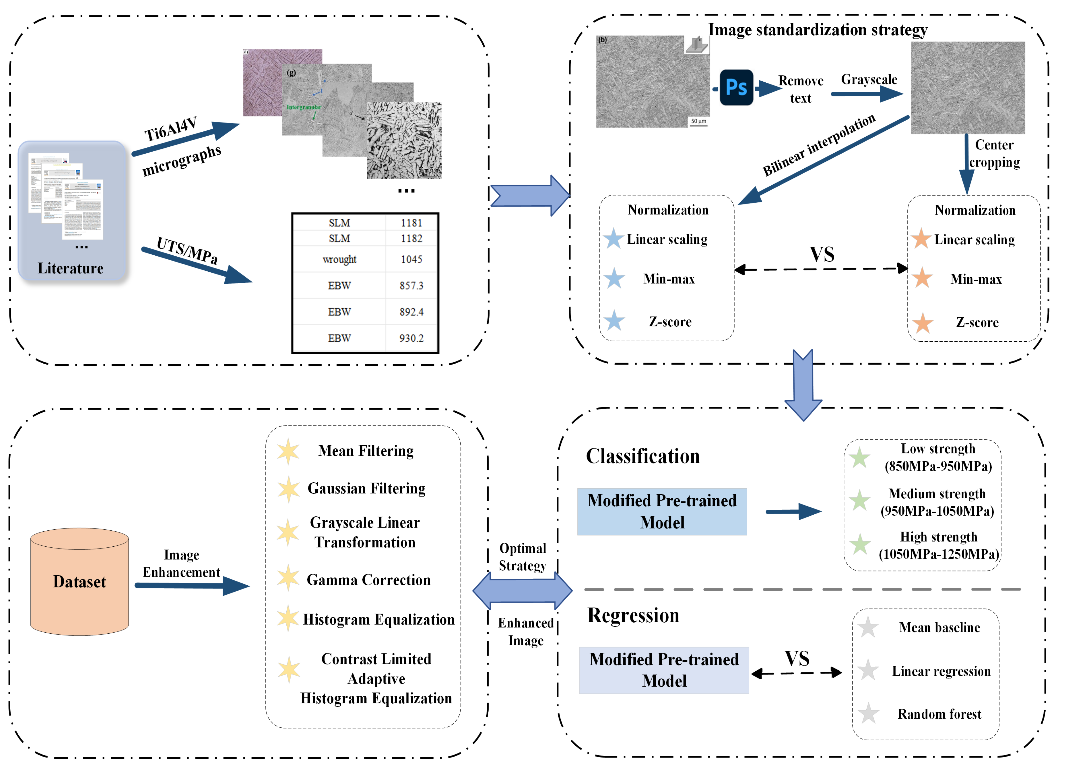
2. Materials and Methods

The dataset construction, preprocessing pipeline design, and deep learning model implementation in this study follow the workflow illustrated in Figure 1.

2.1. Data Collection

To avoid overwhelming structural differences, 180 micrographs with similar magnifications were selected to construct the dataset, and the size distribution of each image is detailed in Figure 2a. The corresponding ultimate tensile strength (UTS) data ranged from 850 MPa to 1250 MPa, and Figure 2b presents the specific distribution. The left scatterplot links each micrograph to its specific UTS value, and the histogram (right) shows the frequency distribution of micrographs within defined UTS intervals. The micrographs included traditional manufacturing (e.g., casting, rolling) and additive manufacturing [e.g., Selective Laser Melting (SLM), Electron Beam Melting (EBM), Directed Energy Deposition (DED)] optical micrographs, supplemented with scanning electron microscope (SEM) images for diversity enhancement.

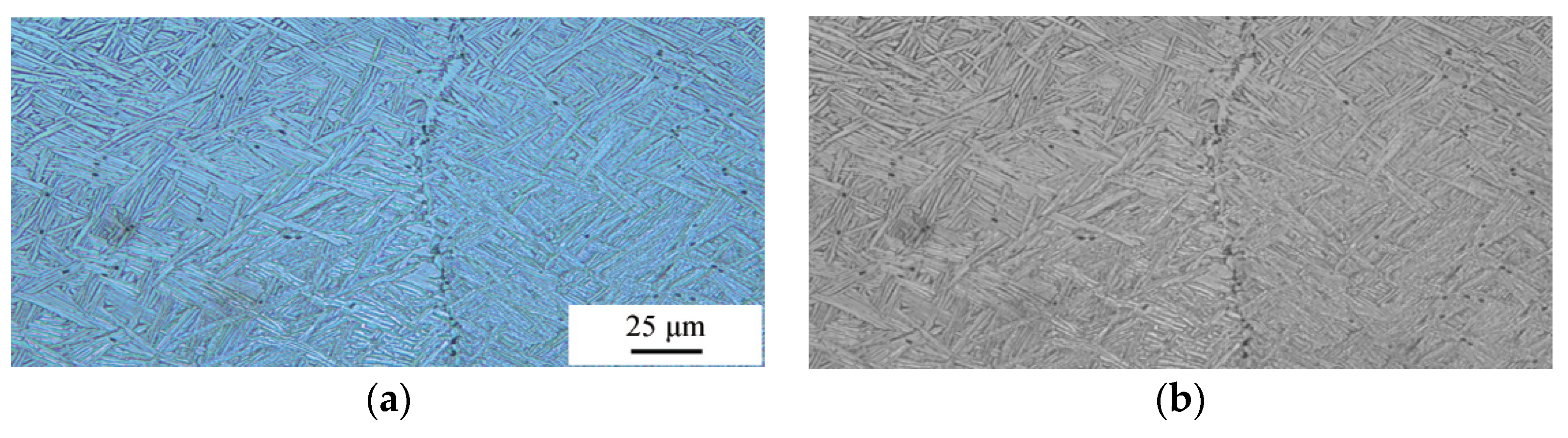
2.2. Image Standardization

2.2.1. Color Processing

As the micrographs were collected from the published literature, Photoshop software (Adobe Photoshop 2024, version 25.0.0, Adobe Inc., San Jose, CA, USA) was used to remove the text and rulers labeled on the images. Furthermore, the inconsistent illumination conditions led to significant color differences among images. A comparative study [13] found that maintaining the original color of the material micrographs does not significantly enhance the performance of the deep learning model. Therefore, to ensure consistency among micrographs, grayscale transformation was applied to all images before model training. The processing effect is shown in Figure 3.

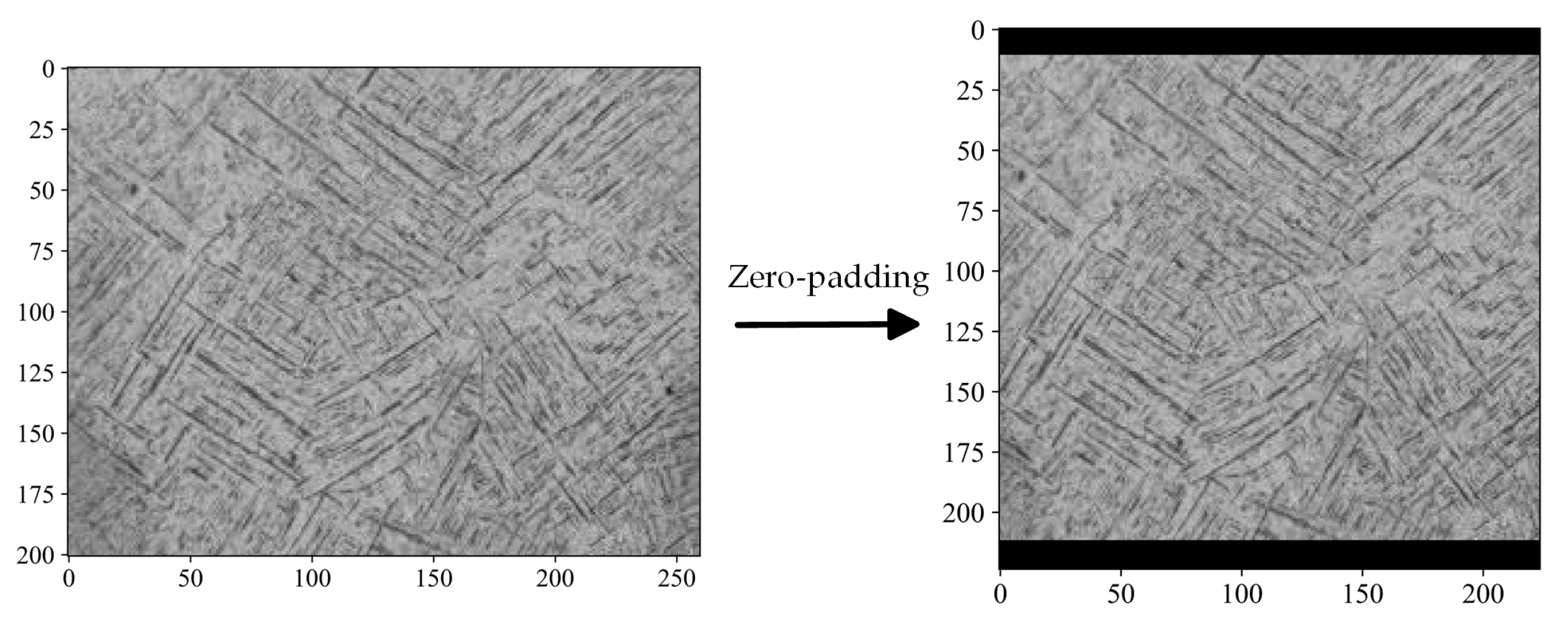
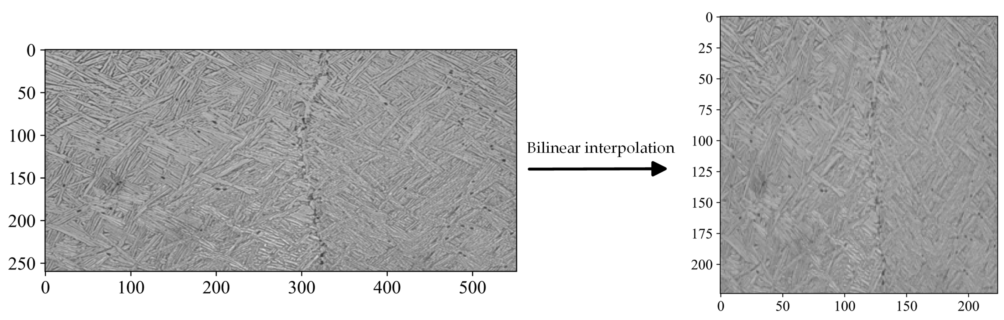
2.2.2. Size Adjustment

During model training, image sizes need to be kept consistent. However, the images in the dataset varied in size. Therefore, center cropping and bilinear interpolation were independently adopted to resize them to 224 × 224.
  • Center cropping
Center cropping resizes an image by cropping its central region. For images smaller than the target size, zero padding is first applied to expand the image, followed by cropping to the target size. Hashemi [14] pointed out that padding with zeros does not reduce the training effect and also improves training speed of the model. The effects of center cropping are shown in Figure 4 and Figure 5.
  • Bilinear interpolation
Bilinear interpolation adjusts the size by scaling the image. When the values and coordinates of the four neighboring pixels are known, bilinear interpolation computes the pixel value at the target position by performing linear interpolation in both horizontal and vertical directions [15]. Assume the scaled pixel corresponds to the original image coordinate (x, y), with four surrounding pixel values denoted as P11, P12, P21, P22, located at integer coordinates (x1, y1), (x1, y2), (x2, y1), and (x2, y2), where x2 = x1 + 1 and y2 = y1 + 1. Bilinear interpolation first performs linear interpolation along the x-axis to calculate intermediate values P1 and P2, as detailed in Equations (1) and (2). The final interpolated pixel value P is then derived through linear interpolation along the y-axis using P1 and P2, as detailed in Equation (3). The effect after scaling is shown in Figure 6.
P 1 = x 2 x x 2 x 1 P 11 + x x 1 x 2 x 1 P 21
P 2 = x 2 x x 2 x 1 P 12 + x x 1 x 2 x 1 P 22
P = y 2 y y 2 y 1 P 1 + y y 1 y 2 y 1 P 2

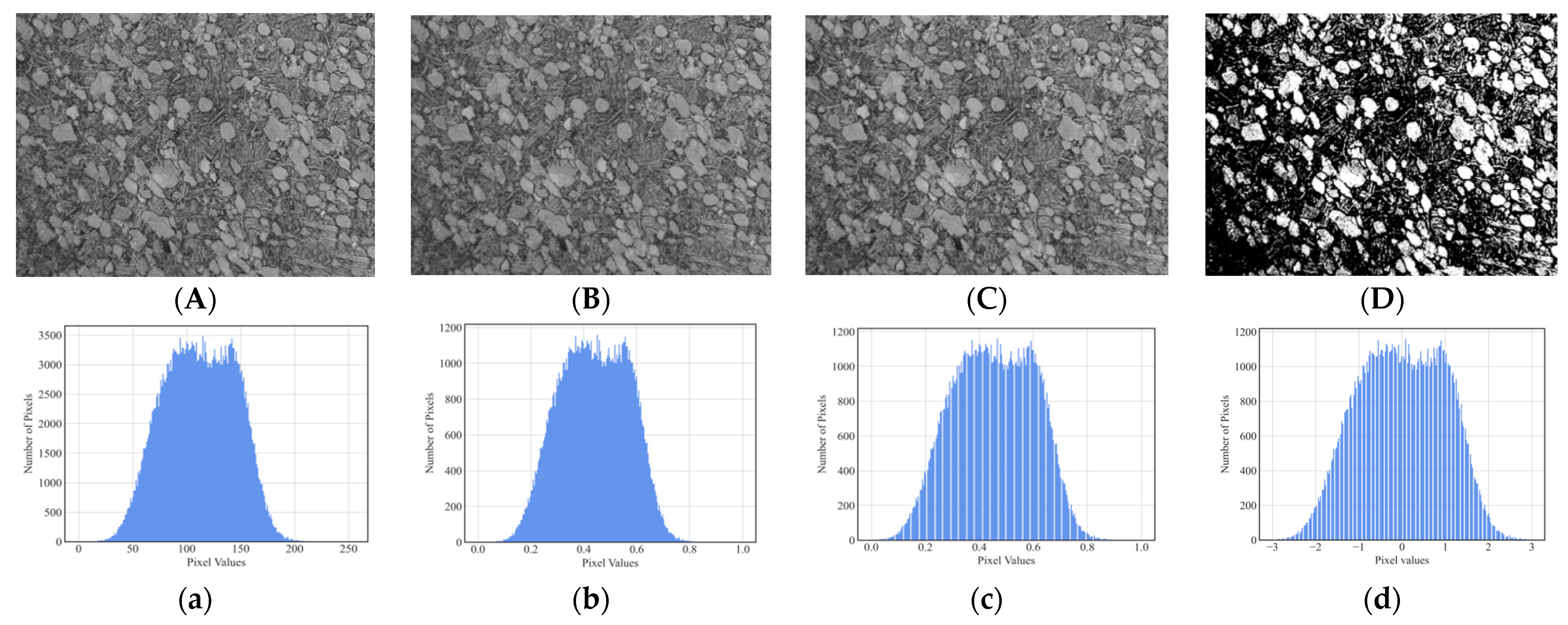
2.2.3. Image Normalization

Image normalization is commonly used to mitigate potential issues of gradient vanishing or explosion, as well as to accelerate model convergence [16]. Distinct normalization methods adjust the distribution of data features in various ways, which may lead to different training outcomes [17]. After applying grayscale and image resizing, three normalization methods were applied to the micrographs dataset independently: linear scaling, min–max normalization, and Z-score normalization.
  • Linear scaling
As the pixel value of grayscale images ranges from [0, 255], a common normalization method is used to divide each pixel value by 255 to linearly scale the data into the [0, 1] range. The linear scaling operation is detailed in Equation (4):
P n o r m = P i 255
where Pnorm denotes the pixel value after normalization, while Pi denotes the original pixel value.
2.
Min–max normalization
Min–max normalization processes each image according to Equation (5):
P n o r m = P i min ( P ) max ( P ) min ( P )
where min(P) and max(P) represent the minimum and maximum pixel values in the image. When min(P) = 0 and max(P) = 255, then min–max normalization simplifies to Equation (4).
3.
Z-score normalization
Z-score normalization processes each image according to Equation (6):
P n o r m = P i μ σ
where μ denotes the mean of the dataset, and σ denotes the standard deviation of the dataset. Z-score normalization computes the mean and standard deviation for each channel across all images in the dataset to perform normalization. The processing effects and corresponding pixel value distributions are shown in Figure 7.
Compared to the original grayscale image, both linear scaling and min–max normalization resulted in minimal visual changes. However, these two methods scaled the pixel value range to [0, 1], and min–max normalization further enhanced uniformity in pixel value distribution. Z-score normalization led to a significant visual shift because the pixel values were scaled to the range [−3, 3], which is outside the displayable range of [0, 1] for OpenCV. Nevertheless, the information stored in the image was not affected by this transformation.

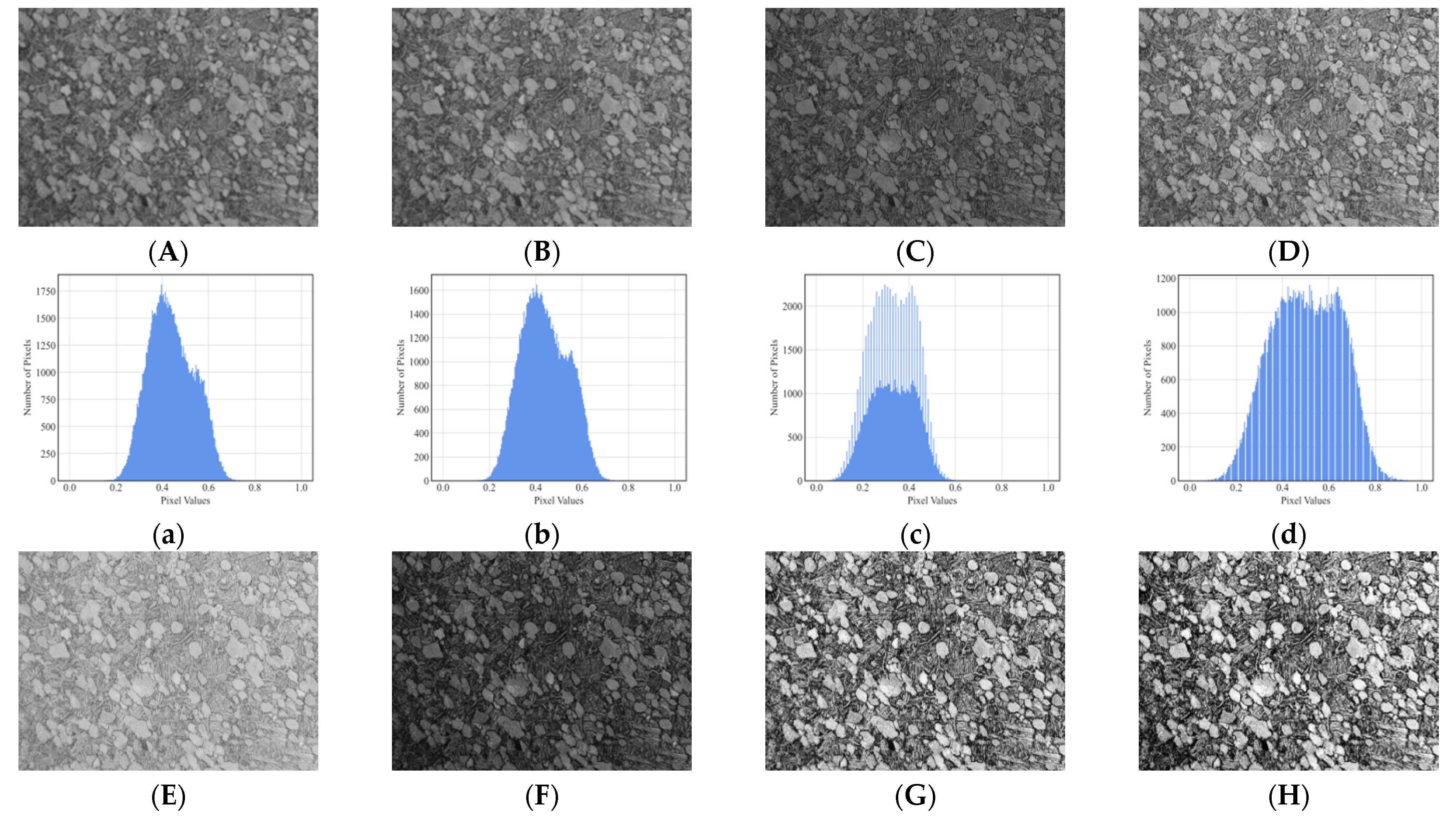
2.3. Image Enhancement

Image enhancement aims to improve image quality by enhancing details and optimizing visual effects. Common methods of image enhancement include contrast enhancement [18], brightness adjustment [19], and other approaches. Following the normalization, a series of image enhancement methods were applied to further evaluate the performance of the model. Table 1 lists the roles and parameters of each method. The effects of the enhancement are shown in Figure 8.
Figure 8A,B,a,b and show that even though MF and GF did not cause significant changes in visual effects, the distribution of pixel values differed from the original. This change occurred because both MF and GF removed potential noise and smoothed the image. Figure 8C,D,c,d correspond to the effects of GLT processing under two different parameter settings. The former (Figure 8C,c) decreased the brightness and contrast by reducing pixel values, while the latter (Figure 8D,d) increased them. Figure 8E,F,e,f correspond to the effects of γ = 0.5 and γ = 1.7. When γ < 1, GC nonlinearly stretched dark regions, enhancing visibility and perceived brightness. When γ > 1, GC compressed highlights, recovering details and improving contrast [20]. Figure 8G,H,g,h correspond to the effects of CLAHE and HE [21]. HE globally equalized the histogram to a near-uniform distribution to achieve contrast enhancement, while CLAHE adaptively constrains local contrast within subregions, producing smoother intensity transitions.

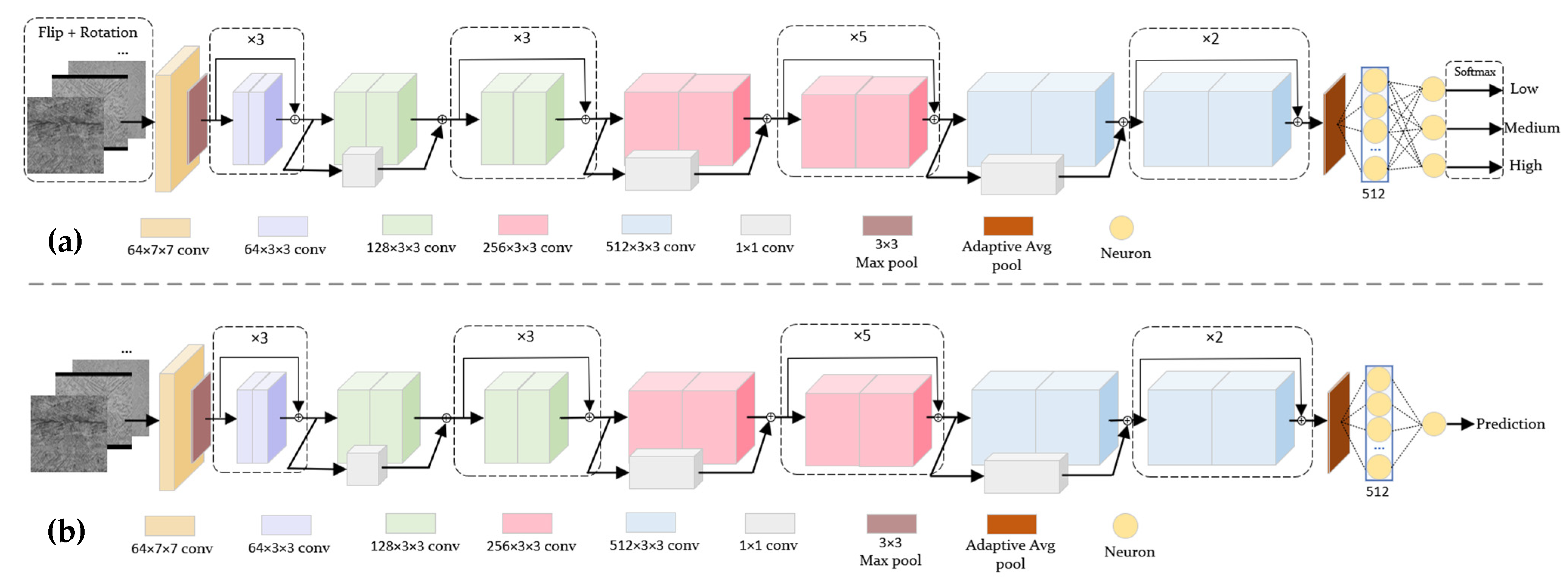
2.4. Models for Classification and Prediction

He et al. [22] introduced the ResNet architecture in 2015, employing residual blocks with shortcut connections to mitigate model degradation in deep networks. This innovation enabled ResNet to win the 2015 ImageNet classification competition. In this paper, a pre-trained ResNet34 model was employed for transfer learning to extract features from micrographs of Ti6Al4V alloy. As an initial step in assessing the model’s predictive capability, a classification task was performed by partitioning the dataset into three discrete strength grades based on UTS magnitude, as detailed in Table 2. To address the mild class imbalance in low-strength samples, data augmentation techniques such as random flipping (horizontal and vertical) and random rotation (degrees = 15) were applied to the training set. The structure of the classification model is illustrated in Figure 9a, where the output layer was reconfigured with three neurons corresponding to the target classes.
In the regression task, as shown in Figure 9b, the ResNet34 architecture was adapted as a CNN-based regression model by modifying its output layer to a single neuron. In addition, to compare the performance of the CNN-based model, three traditional predictive models including mean baseline, linear regression, and random forest were implemented. The mean baseline generates predictions by computing the mean of the training set labels, while both linear regression [23] and random forest [24] produce outputs through fitting image features extracted from the Gray-Level Co-occurrence Matrix (GLCM) [25].
The classification model employed cross-entropy loss function [26] as the loss function, with the calculation formula shown in Equation (7):
L = 1 n i c = 1 M y i c log ( p i c )
where n is the number of samples, M represents the number of categories, yic is the indicator function (1 if sample i’s true class is c, 0 otherwise), pic represents the predicted probability of sample i belonging to class c. The CNN-based regression model used the mean square error (MSE) [27] as the loss function, which is detailed in Equation (8).
To ensure the generalization ability of the model and to mitigate potential biases introduced by random data partitioning, the dataset was divided using 5-fold cross-validation, where each iteration allocated four subsets for training and one used for testing. Details regarding other methodologies and hyperparameter configurations are summarized in Table 3, Table 4 and Table 5, respectively.
The classification model performance was evaluated by the accuracy [28], while the regression model was evaluated by aggregating test set predictions from all cross-validation folds to compute overall coefficient of determination (R2). Furthermore, to minimize the impact of random initialization that may lead to premature convergence, 5-fold cross-validation was conducted five times for each preprocessed dataset. Then, the mean and standard deviation of accuracy and R2 were computed after ruling out outliers. The calculation formula of R2 is detailed in Equation (9).
M S E = 1 n i = 1 n ( y i f ( x i ) ) 2
R 2 = 1 i = 1 n ( f ( x i ) y i ) 2 i = 1 n ( 1 n i = 1 n y i y i ) 2
In the above equations, yi represents the true value corresponding to the i-th image, while f(xi) denotes its predicted value, and n is the number of samples. In this study, PyTorch (version 2.0.0, Meta Platforms, Inc., Menlo Park, CA, USA) was used as the deep learning framework.
Table 3. Methods and hyperparameter configurations for the classification model.
Method and HyperparameterConfiguration
OptimizerAdam
Epoch200
Early stop patience [29]7
Learning rate0.0001
Batch size8
Initialization of weights in FCXavier uniform
K-fold cross validationK = 5, Shuffle = True, random_state = 42
Table 4. Methods and hyperparameter configurations for the CNN-based regression model.
Method and HyperparameterConfiguration
OptimizerAdam
Epoch200
Early stop patience16
Learning rate0.008
Batch size8
Initialization of weights in FCXavier uniform
K-fold cross validationK = 5, Shuffle = True, random_state = 42
Table 5. Methods and hyperparameter configurations for the traditional predictive model.
Random ForestConfiguration
n_estimators100
Random state42
GLCMdistance[1]
angles[0]
SymmetricTrue
normedTrue
levels256
Extracted featurescontrast
energy
homogeneity
correlation

3. Results

3.1. Test Results of Classification Model

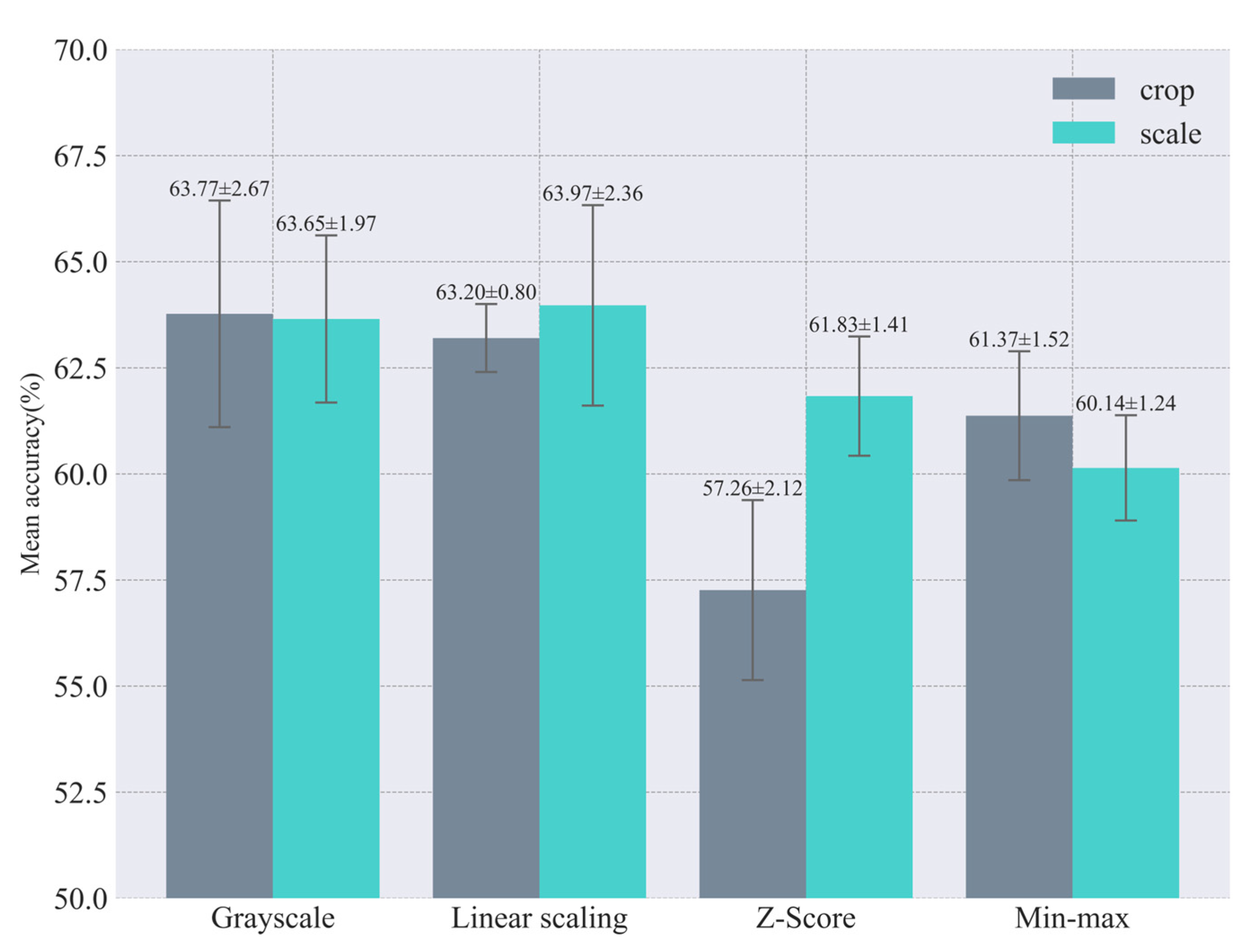
3.1.1. Test Results of Image Standardization

Figure 10 presents the mean accuracy and corresponding standard deviation of the classification model under different image standardization strategies. Compared to the non-normalized data, the mean accuracy was only slightly improved on the dataset processed with interpolation and linear scaling. Other standardization strategies led to performance degradation, particularly for Z-Score normalization and min–max normalization. Based on these results, the subsequent enhancement methods were built upon the combination of linear scaling and bilinear interpolation.

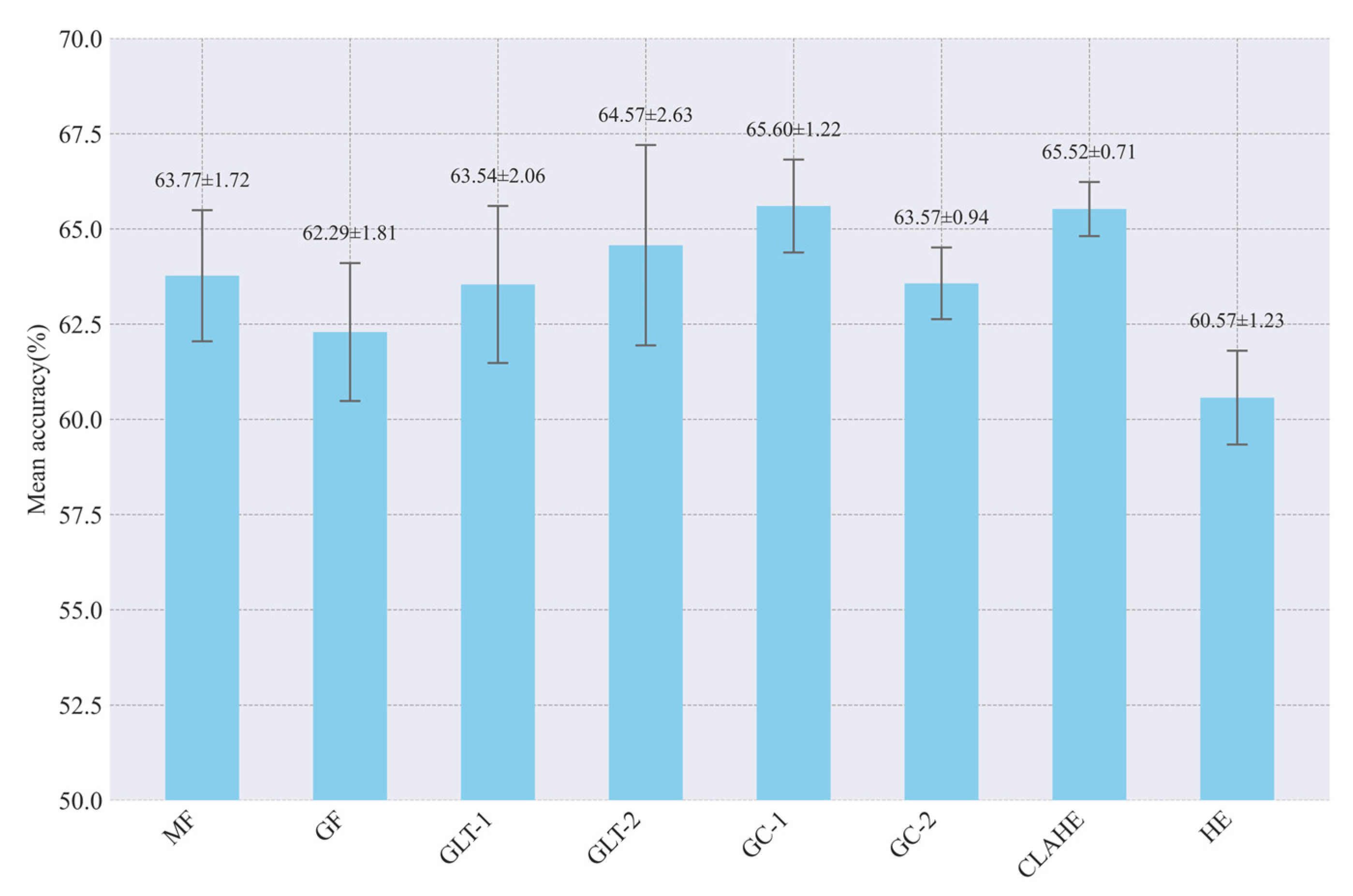
3.1.2. Test Results of Image Enhancement

Figure 11 presents the mean accuracy and corresponding standard deviation of the classification model using different image enhancement methods. Compared to the accuracy in Section 3.1.1 (63.97% ± 2.36%), GC-1 achieved the highest accuracy (65.60% ± 1.22%), followed by CLAHE with comparable performance and lower variability (65.20% ± 0.71%), while GLT-2 showed minimal improvement (64.57% ± 2.63%). However, the application of HE resulted in significant degradation of model performance, demonstrating its unsuitability for the classification task.

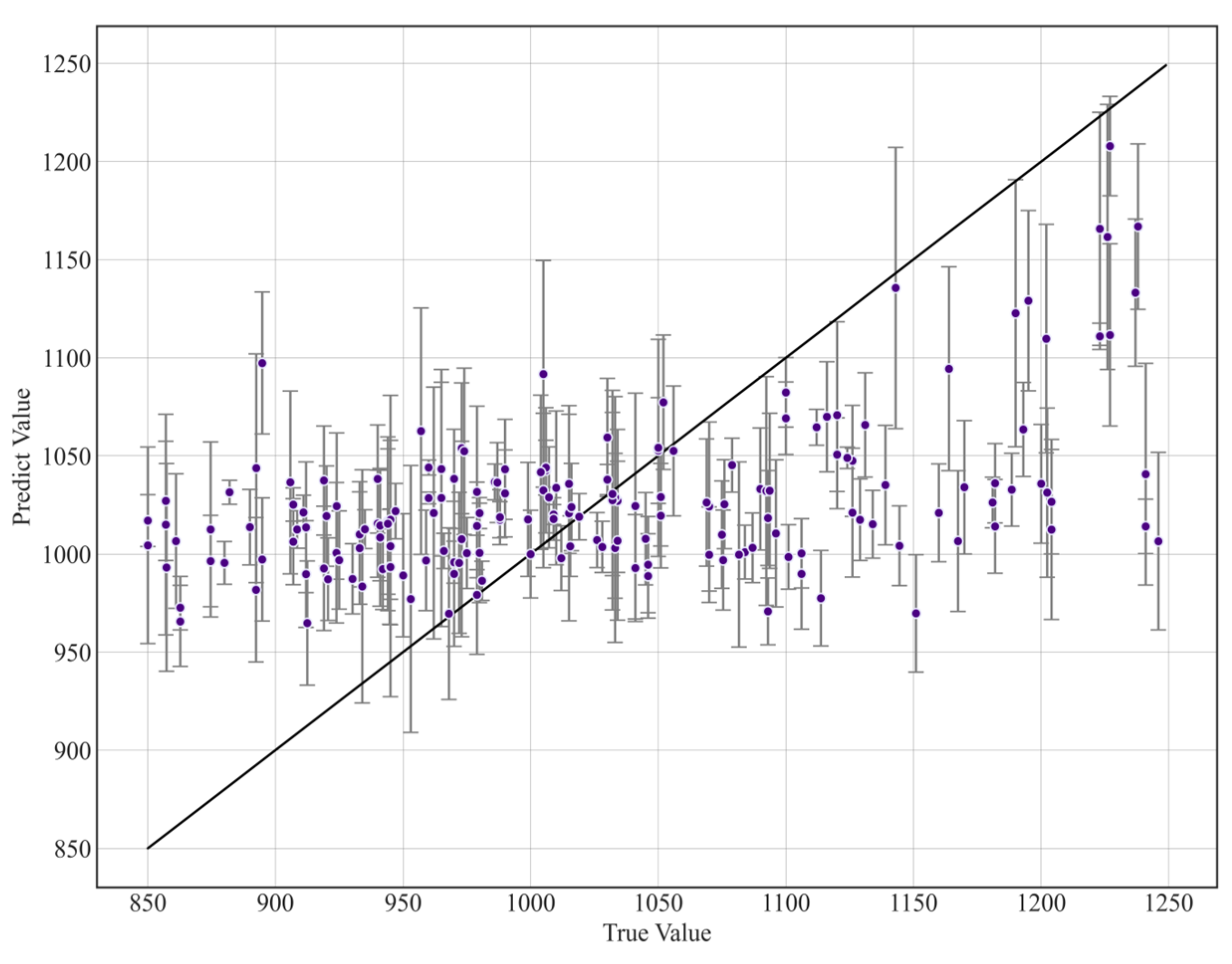
3.2. Test Results of Regression Models

3.2.1. Test Results of Image Standardization

Table 6 and Table 7 present the R2 results of the CNN-based regression model and traditional predictive models on standardized datasets, respectively. Compared to the baseline result (R2 = −0.003), the CNN-based model demonstrated only marginal advantages on non-normalized datasets (R2 = 0.047 ± 0.021 and R2 = 0.026 ± 0.020). The application of normalization methods improved the test results, and the combination of center cropping and min–max normalization yielded the highest R2 value (0.111 ± 0.017). Among the linear regression and random forest models, the random forest achieved the highest R2 (0.1093) on interpolated dataset. However, the inappropriate image resizing method could degrade model performance below baseline level.
These results indicated that both CNN-based models and traditional predictive models exhibited poor predictive capability, with the highest mean R2 reaching only 0.111. This suggested that the models failed to precisely characterize UTS through learning microstructural features when relying only on standardized datasets. Therefore, image enhancement methods were implemented subsequently to enhance image details and further explore model predictive potential. The enhancement methods were built upon the standardization strategies corresponding to each model’s highest R2 in this section.

3.2.2. Test Results of Image Enhancement

Table 8, Table 9 and Table 10 present the R2 results of the CNN-based regression model and traditional predictive models on enhanced datasets. Regrettably, while certain enhancement methods improved test outcomes, the CNN-based models achieved the highest R2 of only 0.163 ± 0.020 (HE-processed dataset), whereas the traditional models attained the highest R2 of 0.139 (yielded by the random forest on GLT-2-processed dataset). As shown in Figure 12, the distribution of predicted values for the CNN-based model on the HE-processed dataset was further visualized by a scatter plot with error bars, calculated from the mean and standard deviation of multiple predictions. The figure shows that most predictions were constrained within a specific UTS interval with significant variability, demonstrating that the models had almost no practical predictive capability.
An explanation of the poor results may stem from the high heterogeneity of the dataset, which mixed micrographs from multiple forming processes. As illustrated in Figure 13, significant morphological evolution of Ti6Al4V alloy microstructures might arise due to the phase transformations driven by different processing conditions. These variations introduce high feature complexity, hindering the models’ ability to capture microstructural features that reliably correlate with UTS. Therefore, the next tests focused on creating subsets with less heterogeneity to explore model performance.

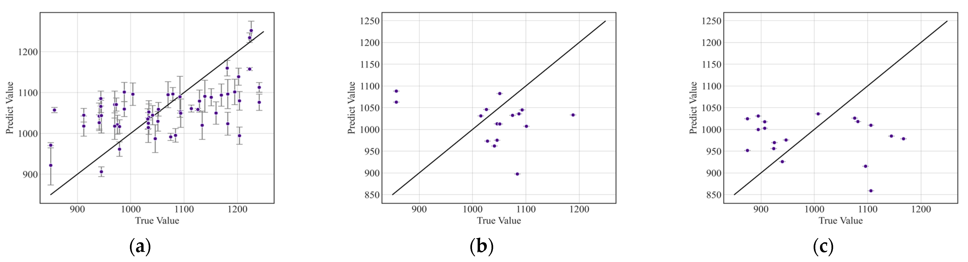
3.2.3. Test Results of Subsets with Less Heterogeneity

To reduce heterogeneity, the subsets were constructed by selecting micrographs with consistent forming processes from the dataset. Based on the previous results comparison, this section analyzed the predictive capability of the CNN-based model on HE-processed subset and the random forest on GLT-2 subset. To address limited sample sizes in subsets, the training strategy of the CNN-based model was modified as follows: A subset was isolated from the original dataset, and pre-trained weights were obtained using remaining micrographs for initial training. Subsequently, the subset was fine-tuned with reduced learning rates.
As presented in Table 11 and Table 12, three subsets were employed to evaluate the performance of the model. The results demonstrate that learning micrographs with less heterogeneity improved the test R2 of the CNN-based model, with the highest value of 0.360 achieved after fine-tuning on the DED-based subset. Furthermore, as shown in Figure 14b,c, fine-tuning with subsets containing fewer samples significantly enhanced the model’s predictive stability. In contrast, the random forest exhibited no significant improvement, yielding a maximum R2 of only 0.148.

4. Discussion

4.1. Predictive Capability of the Model

In the classification task, the model achieved a maximum accuracy of 65.60% ± 1.22%, demonstrating its moderate capability in qualitatively classifying strength grades from highly heterogeneous micrographs. However, for the regression task, both CNN-based and traditional models exhibited almost no predictive capability on the dataset (highest R2 = 0.163 ± 0.020). Fine-tuning the CNN-based model on subsets could improve performance. The model fine-tuning on the DED-based subset yielded a peak R2 of 0.360 ± 1.47 × 10⁻5. This suggested that the model was better suited in learning micrographs derived from consistent forming process, as the microstructural variations were relatively small. In contrast, the random forest showed slight improvement on subsets (highest R2 = 0.148), indicating the CNN-based model has better predictive potential on datasets with less heterogeneity.
Despite these improvements, the R2 values were still not ideal. This may arise from different post-processing methodologies across studies, which introduced microstructural heterogeneity even though the alloys were formed in consistent processes, as shown in Figure 15. Additionally, Tsutsui et al. [30] demonstrated that differences in microscopy instruments can induce image feature shifts, further compromising model performance. Therefore, constructing datasets with Ti6Al4V micrographs derived from similar experimental conditions may enhance predictive capability.

4.2. Impact of Size Adjustment and Normalization Methods on Model Performance

In the classification task, no normalization method improved model performance on the cropped dataset, whereas only linear scaling enhanced performance on the interpolated dataset. This suggests that the classification model was not sensitive to normalization. Conversely, normalization methods universally improved regression performance, with the combination of min–max normalization and center-cropping achieving optimal standardization. This indicates that the selection of normalization should depend on both the resizing method and the task type.

4.3. Impact of Image Enhancement Methods on Model Performance

In the classification task, GC-1, CLAHE, and GLT-2 improved model performance, with the highest accuracy achieved on the GC-1-processed dataset. These three methods all aimed to enhance image brightness and detail. However, despite HE also being implemented to enhance contrast, it failed to improve model performance. This may be because HE enhances global contrast, potentially amplifying details unrelated to strength grade classification.
For the regression task, the CNN-based model performed best on HE-processed datasets, followed by GF and MF. The improvements from MF and GF suggest the presence of noise affecting regression performance, as shown in Figure 16. GF outperformed MF, likely because GF employs weighted averaging [31], which reduces the influence of distant pixels on the center pixel to preserve image information, whereas MF relies on local averaging that may blur details. Unlike the classification model, the regression model benefited more from HE-processed datasets. This suggests that the CNN-based model tends to learn globally enhanced microstructural features, while the classification model focuses on amplified local information.
In summary, the classification model benefited from brightness enhancement and localized contrast amplification, whereas the regression model achieved optimal performance with global contrast enhancement, followed by denoising and smoothing techniques.

5. Conclusions

This study presents a systematic evaluation of the predictive capability of a CNN-based deep learning model for the UTS of Ti6Al4V alloy using preprocessed micrographs, and it analyzes the impact of different image preprocessing combinations on model performance. On highly heterogeneous datasets, the model exhibited moderate capability in quantitatively classifying strength grades from micrographs (accuracy = 65.60% ± 1.22%) but negligible UTS regression capability (highest R2 = 0.163 ± 0.020). It is more appropriate to conduct the regression task using micrographs obtained under similar experimental conditions: The model fine-tuned on a subset with consistent forming process demonstrated improved performance (highest R2 = 0.360 ± 1.47 × 10⁻⁵), outperforming traditional predictive models.
During standardization, the normalization selection should be matched to the specific image resizing method and task type: classification model was not sensitive to normalization, while normalization methods universally improved regression performance, with the min–max normalization and center-cropping combination achieving optimal standardization. Among image enhancement methods, gamma correction most effectively improved classification accuracy, while histogram equalization delivered optimal regression performance. The classification model performed better on datasets processed by brightness enhancement and localized contrast amplification, while the regression model benefited most from global contrast enhancement, followed by denoising and smoothing.
Overall, this research aids the researchers in selecting appropriate data preparation strategies and preprocessing approaches when applying machine learning to predict mechanical properties of Ti6Al4V alloys through micrograph analysis.

Author Contributions

Conceptualization, Y.X. and W.D.; methodology, software, validation, formal analysis, investigation, resources, data curation, visualization, writing—original draft preparation, Y.X.; writing—review and editing, supervision, project administration, funding acquisition, W.D. All authors have read and agreed to the published version of the manuscript.

Funding

This research was funded by the National Natural Science Foundation of China (Grant No. 52175359).

Data Availability Statement

The raw data supporting the conclusions of this article will be made available by the authors on request.

Conflicts of Interest

The authors declare no conflicts of interest.

References

  1. Goyal, V.; Prasad, N.K.; Verma, G. Experimental investigations into corrosion behaviour of DMLS manufactured Ti6Al4V alloy in different biofluids for orthopedic implants. Mater. Today Commun. 2025, 42, 111158. [Google Scholar] [CrossRef]
  2. Nagalingam, A.P.; Gopasetty, S.K.; Wang, J.; Yuvaraj, H.K.; Gopinath, A.; Yeo, S.H. Comparative fatigue analysis of wrought and laser powder bed fused Ti-6Al-4V for aerospace repairs: Academic and industrial insights. Int. J. Fatigue 2023, 176, 107879. [Google Scholar] [CrossRef]
  3. Liu, S.; Shin, Y.C. Additive manufacturing of Ti6Al4V alloy: A review. Mater. Des. 2019, 164, 107552. [Google Scholar] [CrossRef]
  4. Cheng, D.; Gao, F. Research Progress and Application of Laser Welding Technology for Titanium Alloy. Dev. Appl. Mater. 2020, 35, 87–93. [Google Scholar] [CrossRef]
  5. Shi, X.; Zeng, W.; Sun, Y.; Han, Y.; Zhao, Y.; Guo, P. Microstructure-Tensile Properties Correlation for the Ti-6Al-4V Titanium Alloy. J. Mater. Eng. Perform. 2015, 24, 1754–1762. [Google Scholar] [CrossRef]
  6. LeCun, Y.; Bengio, Y.; Hinton, G. Deep learning. Nature 2015, 521, 436–444. [Google Scholar] [CrossRef] [PubMed]
  7. Wang, H.; Li, B.; Zhang, W.; Xuan, F. Microstructural feature-driven machine learning for predicting mechanical tensile strength of laser powder bed fusion (L-PBF) additively manufactured Ti6Al4V alloy. Eng. Fract. Mech. 2024, 295, 109788. [Google Scholar] [CrossRef]
  8. Yang, Z.; Yang, M.; Sisson, R.; Li, Y.; Liang, J. A machine-learning model to predict tensile properties of Ti6Al4V parts prepared by laser powder bed fusion with hot isostatic pressing. Mater. Today Commun. 2022, 33, 104205. [Google Scholar] [CrossRef]
  9. Shen, T.; Zhang, W.; Li, B. Machine learning-enabled predictions of as-built relative density and high-cycle fatigue life of Ti6Al4V alloy additively manufactured by laser powder bed fusion. Mater. Today Commun. 2023, 37, 107286. [Google Scholar] [CrossRef]
  10. Zhao, X.; Wang, L.; Zhang, Y.; Han, X.; Deveci, M.; Parmar, M. A review of convolutional neural networks in computer vision. Artif. Intell. Rev. 2024, 57, 99. [Google Scholar] [CrossRef]
  11. Manjunath, J.; Mohana; Madhulika, M.S.; Divya, G.D.; Meghana, R.K.; Apoorva, S. Feature Extraction using Convolution Neural Networks (CNN) and Deep Learning. In Proceedings of the 2018 3rd IEEE International Conference on Recent Trends in Electronics, Information & Communication Technology (RTEICT), Bangalore, India, 18–19 May 2018; pp. 2319–2323. [Google Scholar] [CrossRef]
  12. Murakami, Y.; Furushima, R.; Shiga, K.; Miyajima, T.; Omura, N. Mechanical property prediction of aluminium alloys with varied silicon content using deep learning. Acta Mater. 2025, 286, 120683. [Google Scholar] [CrossRef]
  13. Pei, X.; Zhao, Y.; Chen, L.; Guo, Q.; Duan, Z.; Pan, Y.; Hou, H. Robustness of machine learning to color, size change, normalization, and image enhancement on micrograph datasets with large sample differences. Mater. Des. 2023, 232, 112086. [Google Scholar] [CrossRef]
  14. Hashemi, M. Enlarging smaller images before inputting into convolutional neural network: Zero-padding vs. interpolation. J. Big Data 2019, 6, 98. [Google Scholar] [CrossRef]
  15. Bilal, M.; Ullah, Z.; Mujahid, O.; Fouzder, T. Fast Linde–Buzo–Gray (FLBG) Algorithm for Image Compression through Rescaling Using Bilinear Interpolation. Imaging 2024, 10, 124. [Google Scholar] [CrossRef] [PubMed]
  16. Huang, L.; Qin, J.; Zhou, Y.; Zhu, F.; Liu, L.; Shao, L. Normalization Techniques in Training DNNs: Methodology, Analysis and Application. IEEE Trans. Pattern Anal. Mach. Intell. 2023, 45, 10173–10196. [Google Scholar] [CrossRef] [PubMed]
  17. Albert, S.; Wichtmann, B.D.; Zhao, W.; Maurer, A.; Hesser, J.; Attenberger, U.I.; Schad, L.R.; Zöllner, F.G. Comparison of Image Normalization Methods for Multi-Site Deep Learning. Appl. Sci. 2023, 13, 8923. [Google Scholar] [CrossRef]
  18. Kuran, U.; Kuran, E.C. Parameter selection for CLAHE using multi-objective cuckoo search algorithm for image contrast enhancement. Intell. Syst. Appl. 2021, 12, 200051. [Google Scholar] [CrossRef]
  19. Wang, H.; Yan, X.; Hou, X.; Li, J.; Dun, Y.; Zhang, K. Division gets better: Learning brightness-aware and detail-sensitive representations for low-light image enhancement. Knowl. -Based Syst. 2024, 299, 111958. [Google Scholar] [CrossRef]
  20. Sahnoun, M.; Kallel, F.; Dammak, M.; Mhiri, C.; Mahfoudh, K.B.; Hamida, A.B. A comparative study of MRI contrast enhancement techniques based on Traditional Gamma Correction and Adaptive Gamma Correction: Case of multiple sclerosis pathology. In Proceedings of the 2018 4th Inter-national Conference on Advanced Technologies for Signal and Image Processing (ATSIP), Sousse, Tunisia, 21–24 March 2018; pp. 1–7. [Google Scholar] [CrossRef]
  21. Azizah, L.M.; Kanafiah, S.N.A.B.M.; Jusman, Y.; Raof, R.A.A.; Zin, A.A.M.; Mashor, M.Y. Performance of the H-Butterworth, CLAHE, and HE Methods for Adenocarcinoma Images. In Proceedings of the 2024 International Conference on Information Technology and Computing (ICITCOM), Yogyakarta, Indonesia, 7–8 August 2024; pp. 301–305. [Google Scholar] [CrossRef]
  22. He, K.; Zhang, X.; Ren, S.; Sun, J. Deep Residual Learning for Image Recognition. In Proceedings of the 2016 IEEE Conference on Computer Vision and Pattern Recognition (CVPR), Las Vegas, NV, USA, 27–30 June 2016; pp. 770–778. [Google Scholar] [CrossRef]
  23. Huang, M. Theory and Implementation of linear regression. In Proceedings of the 2020 International Conference on Computer Vision, Image and Deep Learning (CVIDL), Chongqing, China, 10–12 July 2020; pp. 210–217. [Google Scholar] [CrossRef]
  24. Breiman, L. Random forests. Mach. Learn. 2001, 45, 5–32. [Google Scholar] [CrossRef]
  25. Kurniati, F.T.; Sembiring, I.; Setiawan, A.; Setyawan, I.; Huizen, R.R. GLCM-based feature combination for extraction model optimization in object detection using machine learning. J. Ilm. Tek. Elektro Komput. Informatika. 2023, 9, 1196–1205. [Google Scholar] [CrossRef]
  26. Mao, A.; Mohri, M.; Zhong, Y. Cross-Entropy Loss Functions: Theoretical Analysis and Applications. In Proceedings of the International Conference on Machine Learning, PMLR, Honolulu, HI, USA, 23–29 July 2023; pp. 23803–23828. [Google Scholar]
  27. Elharrouss, O.; Mahmood, Y.; Bechqito, Y.; Serhani, M.A.; Badidi, E. Loss Functions in Deep Learning: A Comprehensive Review. arXiv 2025, arXiv:2504.04242. [Google Scholar]
  28. Foody, G.M. Challenges in the real world use of classification accuracy metrics: From recall and precision to the Matthews correlation coefficient. PLoS ONE 2023, 18, e0291908. [Google Scholar] [CrossRef] [PubMed]
  29. Domingo, R.A.; Martínez-Fernández, S.; Verdecchia, R. Energy efficient neural network training through runtime layer freezing, model quantization, and early stopping. Comput. Stand. Interfaces 2025, 92, 103906. [Google Scholar] [CrossRef]
  30. Tsutsui, K.; Terasaki, H.; Uto, K.; Maemura, Y.; Hiramatsu, S.; Hayashi, K.; Moriguchi, K.; Morito, S. A methodology of steel microstructure recognition using SEM images by machine learning based on textural analysis. Mater. Today Commun. 2020, 25, 101514. [Google Scholar] [CrossRef]
  31. Hai, X.; Cao, S.; Cui, S.; Ma, J.; Gao, K. Image Filter Processing Algorithm Analysis and Comparison. J. Phys. Conf. Ser. 2021, 1820, 012192. [Google Scholar] [CrossRef]
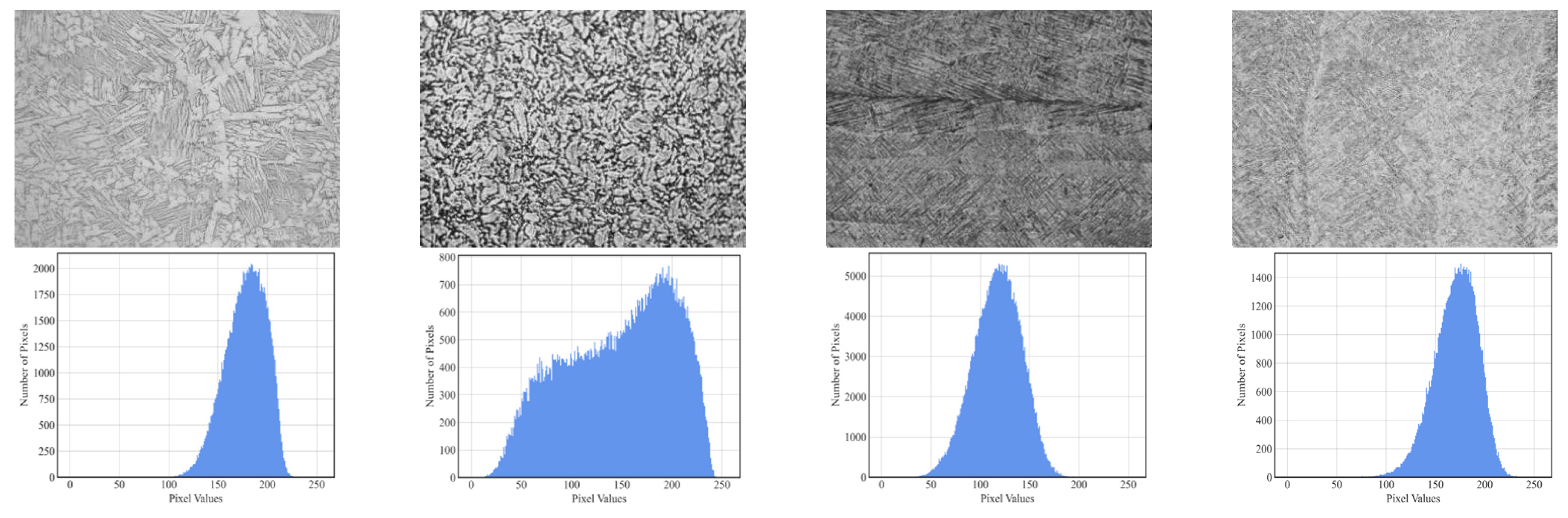
Figure 1. Workflow of dataset construction, preprocessing pipeline design, and deep learning model implementation.
Metals 15 00586 g001
Figure 2. (a) Size distribution of images; (b) distribution of ultimate tensile strength.
Metals 15 00586 g002
Figure 3. A comparison of the original image and grayscale image: (a) original image; (b) grayscale image.
Metals 15 00586 g003
Figure 4. Center cropping when the image size is larger than 224 × 224.
Metals 15 00586 g004
Figure 5. Center cropping when the image height is smaller than 224.
Metals 15 00586 g005
Figure 6. Effect after bilinear interpolation.
Metals 15 00586 g006
Figure 7. (A,a): original grayscale image and the corresponding pixel value distribution; (B,b): grayscale image and the corresponding pixel value distribution after linear scaling; (C,c): grayscale image and the corresponding pixel value distribution after min–max normalization; (D,d): grayscale image and the corresponding pixel value distribution after Z-score normalization.
Metals 15 00586 g007
Figure 8. (A,a): MF and the corresponding pixel value distribution; (B,b): GF and the corresponding pixel value distribution; (C,c): GLT-1 and the corresponding pixel value distribution; (D,d): GLT-2 and the corresponding pixel value distribution; (E,e): GC-1 and the corresponding pixel value distribution; (F,f): GC-2 and the corresponding pixel value distribution; (G,g): CLAHE and the corresponding pixel value distribution; (H,h): HE and the corresponding pixel value distribution.
Metals 15 00586 g008aMetals 15 00586 g008b
Figure 9. (a) Model for classification. (b) Model for prediction.
Metals 15 00586 g009
Figure 10. Results under different image standardization strategies.
Metals 15 00586 g010
Figure 11. Results after using different image enhancement methods.
Metals 15 00586 g011
Figure 12. Prediction results of the CNN-based model on HE-processed dataset. The scatter points indicate the mean predicted values, while the diagonal reference line (y = x) serves as the baseline to evaluate discrepancies between predicted and true values.
Metals 15 00586 g012
Figure 13. Diverse microstructures in grayscale micrographs and the corresponding pixel value distributions.
Metals 15 00586 g013
Figure 14. Prediction results of the CNN-based regression model on (a) SLM-based subset; (b) DED-based subset; (c) EBM-based subset. The scatter points indicate the mean predicted values, while the diagonal reference line (y = x) serves as the baseline to evaluate discrepancies between predicted and true values.
Metals 15 00586 g014
Figure 15. Micrographs from different studies in SLM-based subset.
Metals 15 00586 g015
Figure 16. A comparison of (a) original grayscale image; (b) grayscale image processed by MF; (c) grayscale image processed by GF.
Metals 15 00586 g016
Table 1. Roles and parameters of each image enhancement method.
MethodRoleParameters
Mean Filtering (MF)Remove noise and smooth imageKsize = (3,3) (Based on OpenCV)
Gaussian Filtering (GF)Remove noise and smooth imageKsize = (3,3), sigmaX = 0 (Based on OpenCV)
Gray Linear Transformation-1 (GLT-1)Reduce brightness and contrastY = kx + b, x represents pixel value, k = 0.75, b = 0
Gray Linear Transformation-2 (GLT-2)Increase brightness and contrastY = kx + b, k = 1.15, b = 0
Gamma Correction-1 (GC-1)Increase brightness and highlight dark detailsY = xγ, x is divided by 255, x ∈ [0, 1]. γ = 0.5
Gamma Correction-2 (GC-2)Reduce brightness and highlight bright detailsY = xγ, x ∈ [0, 1]. γ = 1.7
Contrast Limited Adaptive Histogram Equalization (CLAHE)Enhance local contrasts of the imageclipLimit = 2.0, titleGridsize = (4,4) (Based on OpenCV)
Histogram Equalization (HE)Enhance contrasts and details of the imageDefault parameters (Based on OpenCV)
Table 2. Classification of strength and corresponding sample proportion.
Strength GradeUTS Interval (MPa)Proportion of Samples (%)
Low-strength 850 UTS 950 28
Medium-strength 950 < UTS 1050 35
High-strength 1050 < UTS 1250 37
Table 6. Results of image standardization for CNN-based regression model.
CropScaleLinear ScalingMin–MaxZ-ScoreMean R2Standard Deviation
0.0610.029
0.1110.017
0.0740.018
0.0790.006
0.0610.031
0.1020.026
0.0470.021
0.0260.020
Mean baseline−0.0030
Table 7. Result of image standardization for traditional predictive models.
Linear RegressionRandom ForestCropScaleMean R2
−0.024
0.003
−0.028
0.109
Mean baseline−0.003
Table 8. Results of image enhancement for CNN-based regression model.
MFGFGLT-1GLT2-2GC-1GC-2CLAHEHEMean R2Standard Deviation
0.1170.029
0.1260.017
0.0800.018
0.0580.006
0.1020.031
0.0890.026
0.0710.021
0.1630.020
Mean baseline−0.0030
Table 9. Results of image enhancement for linear regression.
MFGFGLT-1GLT2-2GC-1GC-2CLAHEHEMean R2
0.093
0.082
0.045
0.014
0.052
0.024
−0.086
−0.043
Mean baseline−0.003
Table 10. Results of image enhancement for random forest.
MFGFGLT-1GLT-2GC-1GC-2CLAHEHEMean R2
0.016
0.085
0.111
0.139
−0.021
0.048
−0.016
−0.057
Mean baseline−0.003
Table 11. Results of HE-processed subsets for the CNN-based regression model.
SubsetSample SizeMean R2Standard Deviation
SLM-based560.2980.003
DED-based160.3601.47 × 10−5
EBM-based180.3296.66 × 10−5
Table 12. Results of GLT-2-processed subsets for the random forest.
SubsetSample SizeMean R2
SLM-based560.137
DED-based160.148
EBM-based18-0.233
Disclaimer/Publisher’s Note: The statements, opinions and data contained in all publications are solely those of the individual author(s) and contributor(s) and not of MDPI and/or the editor(s). MDPI and/or the editor(s) disclaim responsibility for any injury to people or property resulting from any ideas, methods, instructions or products referred to in the content.

