Constitutive Model for Hot Deformation Behavior of Fe-Mn-Cr-Based Alloys: Physical Model, ANN Model, Model Optimization, Parameter Evaluation and Calibration

Abstract

The development and validation of constitutive models for high-temperature deformation are critical for bridging microstructure evolution with macroscopic mechanical behavior in materials. In this study, we systematically analyzed the hot deformation behavior of Fe-Mn-Cr-based alloys, compared the modeling processes of physical, phenomenological, and data-driven approaches in detail, and optimized their structural and predictive properties. First, the advantages, disadvantages, and applicability of three traditional models, namely the physical Arrhenius model, the phenomenological Johnson–Cook model, and the artificial neural network (ANN) model, are compared for flow stress prediction. Subsequently, traditional mathematical derivations and numerical optimization methods are evaluated. The parameters and architecture of the ANN model are then systematically optimized using optimization algorithms to enhance training efficiency and prediction accuracy. Finally, sensitivity analysis integrated with Bayesian posterior probability density functions enables the calibration of physical model parameters and uncertainty quantification. The results demonstrate that the ANN with optimized parameters and architecture achieves superior prediction accuracy (R² = 0.9985, AARE = 3.01%) compared to traditional methods. Bayesian inference-based quantification of parameter uncertainty significantly enhances the reliability and interpretability of constitutive model parameters. This study not only reveals the strain–temperature coupling effects in the hot deformation behavior of Fe-Mn-Cr-based alloys but also provides systematic methodological support for constitutive modeling of high-performance alloys and a theoretical foundation for material processing technology design.

1. Introduction

Shape memory alloys (SMAs) occupy a unique position in modern materials science, having been extensively utilized across aerospace, electronics, mechanical engineering, medical fields, and household appliances [1,2,3]. While Ni-Ti alloys currently dominate the commercial market as the most prevalent SMAs, their applications remain constrained by inherent limitations including poor cold workability and expensive raw material [4]. In contrast, Fe-Mn-Si-based shape memory alloys have garnered significant research attention owing to their distinct advantages such as ease of processing, enhanced mechanical strength, excellent cold workability, and cost-effectiveness [5]. These merits have propelled ongoing exploration of their potential for broad industrial implementation [6]. However, the industrial adoption of Fe-Mn-Si SMAs is hindered by challenges in controlling their hot deformation behavior, which is critically influenced by the interplay between thermal processing parameters and initial microstructure [7].

The constitutive model, a key tool for linking microstructure evolution to macroscopic mechanical behavior of materials, plays an irreplaceable role in high-temperature deformation research. Its prediction accuracy directly influences processing optimization and property design. Constitutive models are categorized by scale into three types: Macroscopic Mechanical Models, Microscopic Mechanism Models, and Cross-Scale Models. By modeling methodology, they are further classified as phenomenological models, physical models, and statistical models. Physically driven models, such as the Arrhenius model, are grounded in thermal activation theory. These models capture the coupling between temperature, strain rate, and flow stresses via the Zener–Hollomon parameter [8,9,10,11]. Phenomenological models, such as the Johnson–Cook model, directly fit experimental data through empirical formulas while neglecting microscopic mechanisms. Although they excel in predicting metal flow behavior, their generalization capability is constrained by static empirical parameter assumptions [12,13,14]. In general, traditional models exhibit significant deficiencies in characterizing complex nonlinear relationships, quantifying parameter uncertainties, and coupling multiple mechanisms. These limitations have prompted researchers to explore new approaches that combine microscopic mechanisms with data-driven methods [15,16].

At the same time, the artificial neural network (ANN) provides a novel approach for data-driven constitutive modeling due to its powerful nonlinear mapping capability. Jeong et al. predicted uniaxial tensile flow behavior based on indentation load–depth curves through a combination of finite element simulation and ANN optimization, demonstrating ANN’s potential in extracting complex data relationships [17]. However, traditional ANNs exhibit ‘black-box’ limitations: their hyperparameter selection (e.g., hidden layer structure, activation function) relies on trial and error, and they are prone to overfitting [18,19]. For this reason, the Bayesian method has been integrated to enhance ANN robustness. For instance, Rivera et al. proposed a Gaussian process surrogate model combined with Bayesian inference, which successfully calibrated material strength models under high strain rates [20]. Madireddy et al. optimized the structure and parameters of soft tissue superelastic constitutive models through a Bayesian model selection framework, significantly improving prediction accuracy and generalization ability [21].

In recent years, the Bayesian inference method has emerged as a research focus in materials science, owing to its strengths in uncertainty quantification and model selection [22]. For example, Battalgazy et al. developed a Bayesian optimization-based framework for multi-response constitutive model selection and calibration. By integrating diverse material response data (e.g., stress–strain curves, microstructure evolution), this framework significantly enhanced model reliability under complex operating conditions [23]. Similarly, Ryan et al. employed Bayesian optimization to inversely derive viscoplastic constitutive parameters from high-strain-rate experiments and validated their applicability in armor steel impact simulations, demonstrating the method’s efficiency and robustness in parameter calibration [24]. The Bayesian method provides a systematic framework for multiscale parameter calibration and uncertainty quantification by integrating prior distributions with posterior updates. Despite progress in Bayesian–ANN collaborative modeling, two critical challenges persist: (1) current studies predominantly focus on isolated steps (e.g., parameter calibration or model selection), lacking an integrated framework covering the data-to-validation pipeline [25]; (2) Bayesian–ANN applications in high-temperature deformation of metallic materials remain limited, particularly in modeling complex mechanisms (e.g., strain coupling and dynamic recrystallization), where traditional approaches struggle to reconcile physical interpretability with predictive accuracy [26].

Based on the high-temperature compression test data of the Fe-Mn-Cr alloy, various models were systematically evaluated and parameter uncertainties were quantified using Bayesian inference. Firstly, the advantages and disadvantages of two traditional models and ANN model are compared based on experimental data, and the advantages and disadvantages of traditional mathematical derivation and numerical optimization solution of constitutive model are compared. Subsequently, Bayesian hyperparameter optimization is applied to enhance ANN training efficiency and enable physics-informed parameter calibration. Finally, the uncertainty of the model is quantified through the posterior probability density function. This study aims to develop a high-accuracy, high-reliability methodology for constitutive modeling of high-temperature deformation and to compare the strengths and weaknesses of traditional physical models and purely data-driven models. It also seeks to establish their relationship and provide theoretical support for optimizing material processing technologies.

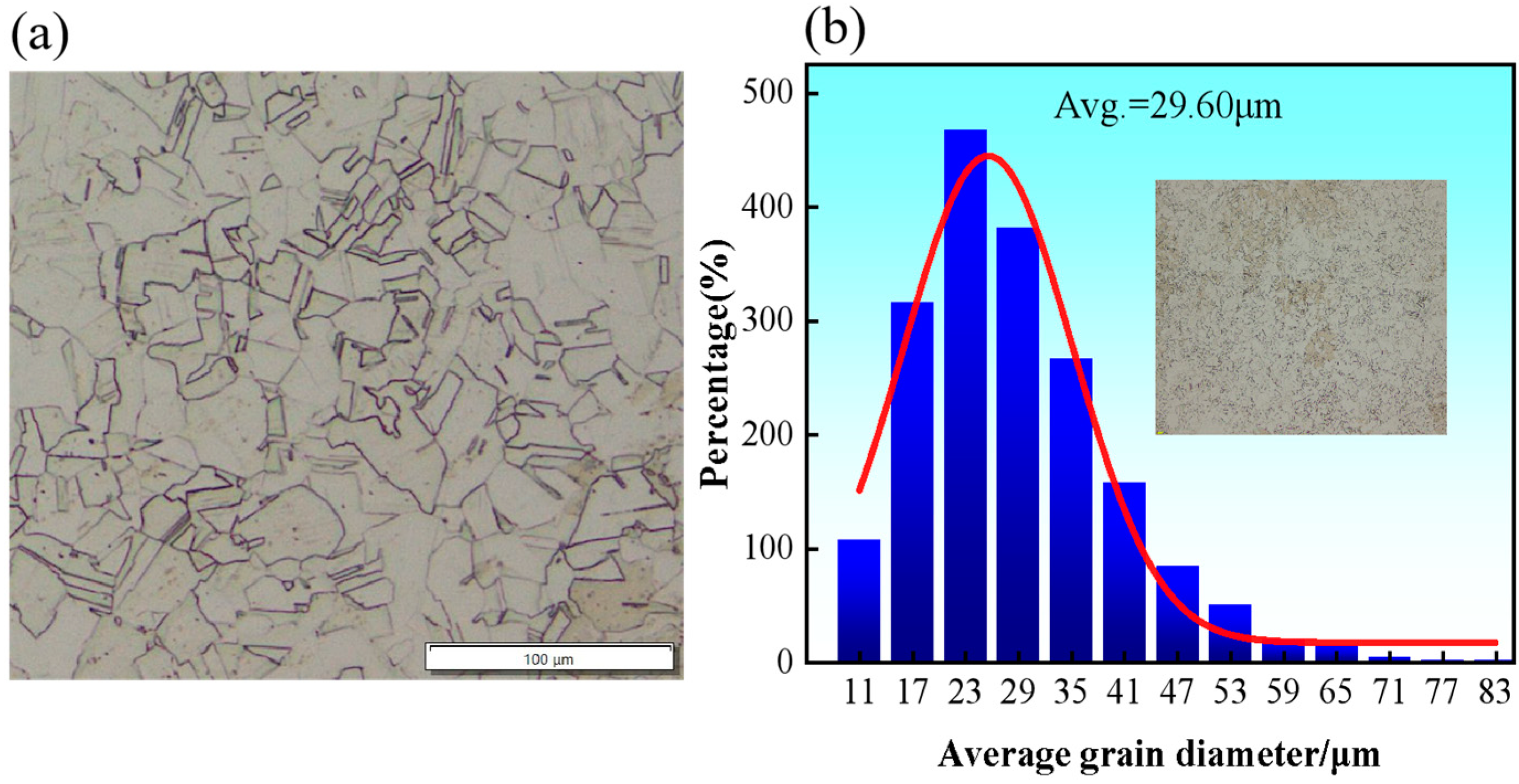
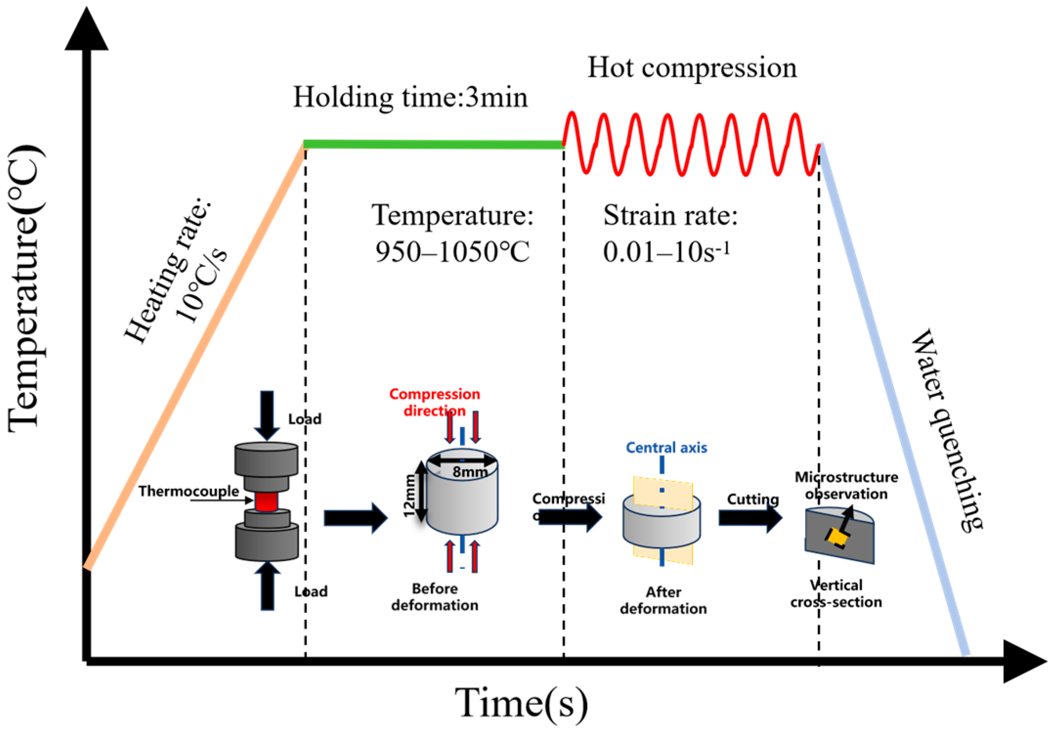
2. Materials and Methods

The Fe66Mn15Si5Cr9Ni5 alloy (chemical composition detailed in

Table 1. Chemical composition of Fe66Mn15Si5Cr9Ni5 alloy (wt%).

Test	Mn	Si	Cr	Ni	Cu	Nb	C	Fe
Fe66Mn15Si5Cr9Ni5	14.78	4.9	9.19	5.1	0.002	0.003	≤0.01	Balance

) was supplied by Changzhou Panxing New Alloy Material Co., Ltd. (Changzhou, China). The alloy was manufactured through industrial-scale processes including casting, forging, hot rolling, and air cooling to obtain initial rod-shaped billets.

The resulting billet exhibits a dual-phase microstructure: γ-Fe (face-centered cubic, FCC) as the primary phase and ε-Fe (hexagonal close-packed, HCP) as a secondary constituent. The initial microstructure displayed an average grain size of 29.6 μm, as determined by the linear-intercept method (Figure 1).

The initial Fe66Mn15Si5Cr9Ni5 blank was machined to obtain a cylindrical specimen with a diameter of 8 mm and a height of 12 mm. The end face of the specimen was polished with 600–2000 # sandpaper to ensure smoothness. Isothermal compression tests were conducted using a Gleeble-1500D thermomechanical simulator sourced from the Department of Mechanical Engineering, Tsinghua University.. The deformation temperatures were 950, 1000, 1050, and 1100 °C, the constant strain rates were 0.01, 0.1, 1, and 10 s⁻¹, respectively, and the compression was set to a constant value of 60%. Before compression, all specimens were heated to the deformation temperature at a rate of 10 °C/s for 3 min to eliminate temperature gradients. Graphite lubricant was applied to the anvil surfaces to minimize interfacial friction during deformation. The schematic diagram of isothermal hot compression test is shown in Figure 2. The test piece was cut along the central axis of the test piece, and the cut part was mechanically ground and polished to a mirror surface. Samples for optical microstructure observation were prepared by chemical etching with a solution of hydrofluoric acid, hydrochloric acid, and pure water at a volume ratio of 1:10:30. An optical microscope (OM) was used to observe the microstructure of the samples.

3. Results

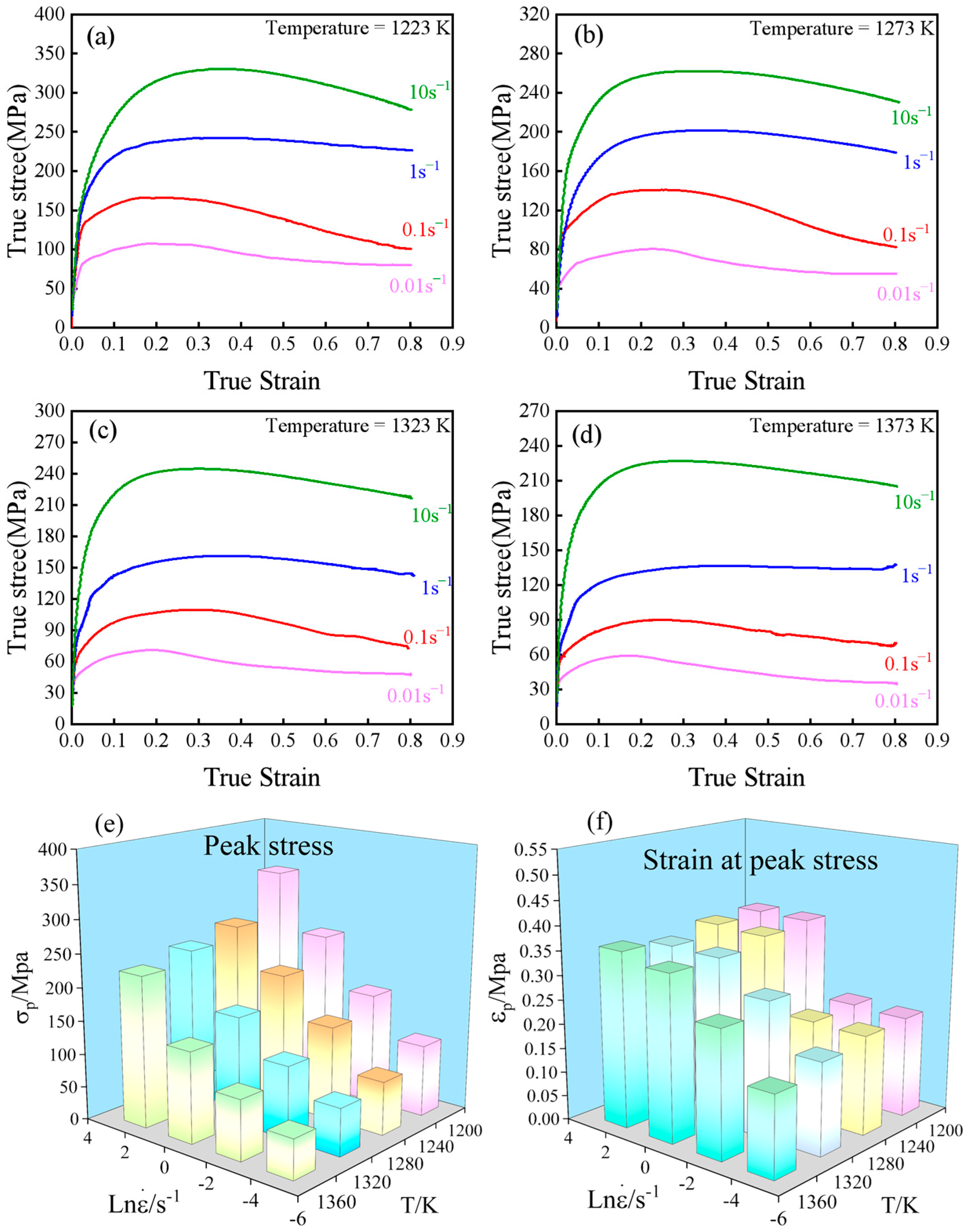
3.1. Flow Behavior

Figure 3 shows stress–strain curves under different conditions, exhibiting three characteristic stages, work hardening, flow softening, and steady-state deformation, which follow a single-peak stress–strain curve pattern [27]. The results clearly demonstrate that peak stress is proportional to strain rate and inversely proportional to temperature. The strain required to reach the peak stress increases with strain rate. For example, at 950 °C, the peak stress increases from 85 MPa at 0.01 s⁻¹ to 210 MPa at 10 s⁻¹, whereas at a strain rate of 10 s⁻¹, the peak stress decreases from 210 MPa at 950 °C to 120 MPa at 1100 °C. This trend is consistent with the evolution of dislocation density: increasing temperature enhances thermal activation energy, inhibits dislocation accumulation, and promotes grain boundary migration, thus strengthening the dynamic softening effect and reducing peak stress. Conversely, higher strain rates lead to higher peak stresses due to shorter deformation times and higher dislocation densities [28,29]. Insufficient annihilation time for high-density dislocation stacking and entanglement, coupled with limited nucleation and growth time for discontinuous dynamic recrystallization (DDRX) grains, increases peak stress and strain required for recrystallization initiation [30].

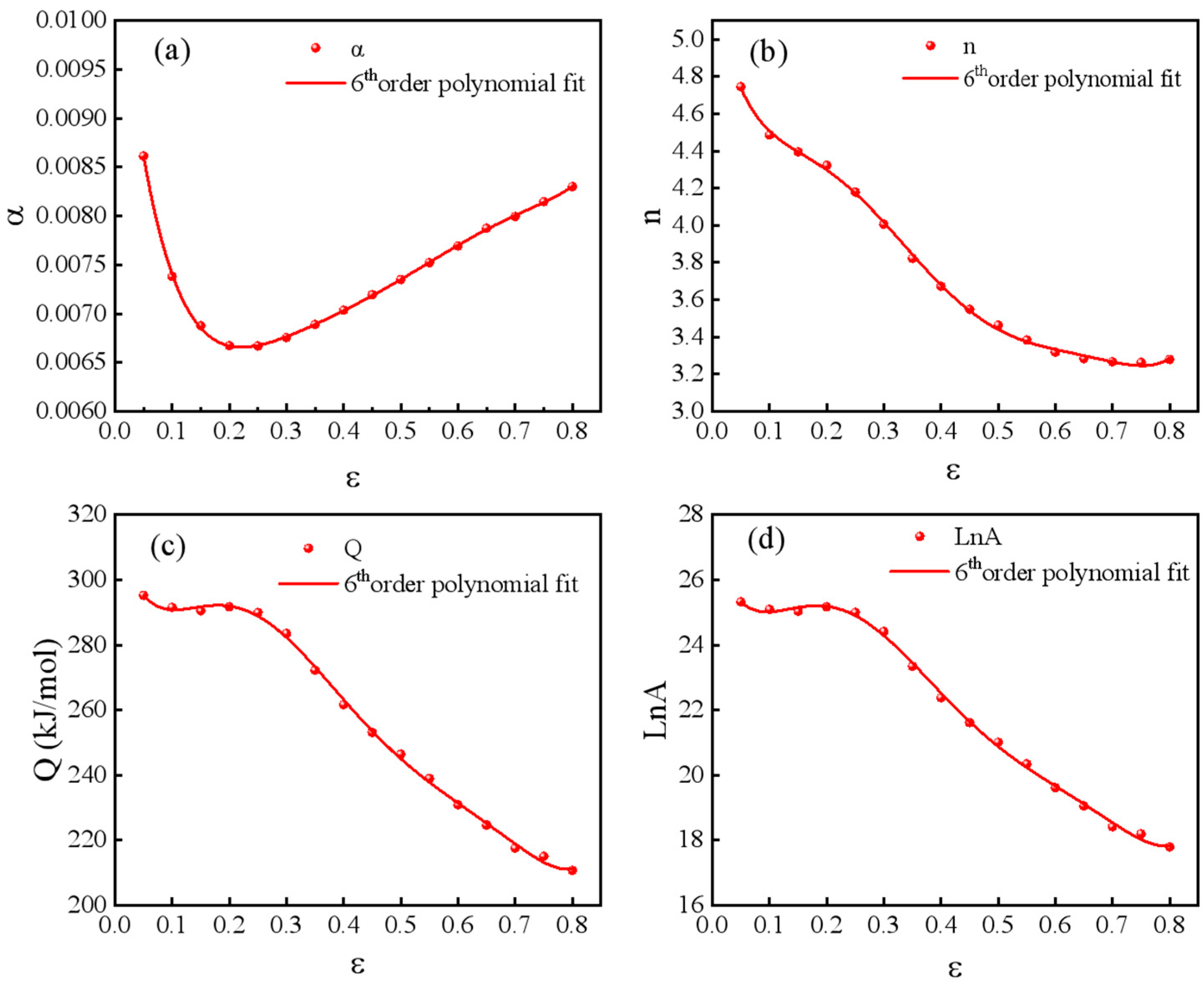
3.2. Establishment and Optimization of Physical Constitutive Models

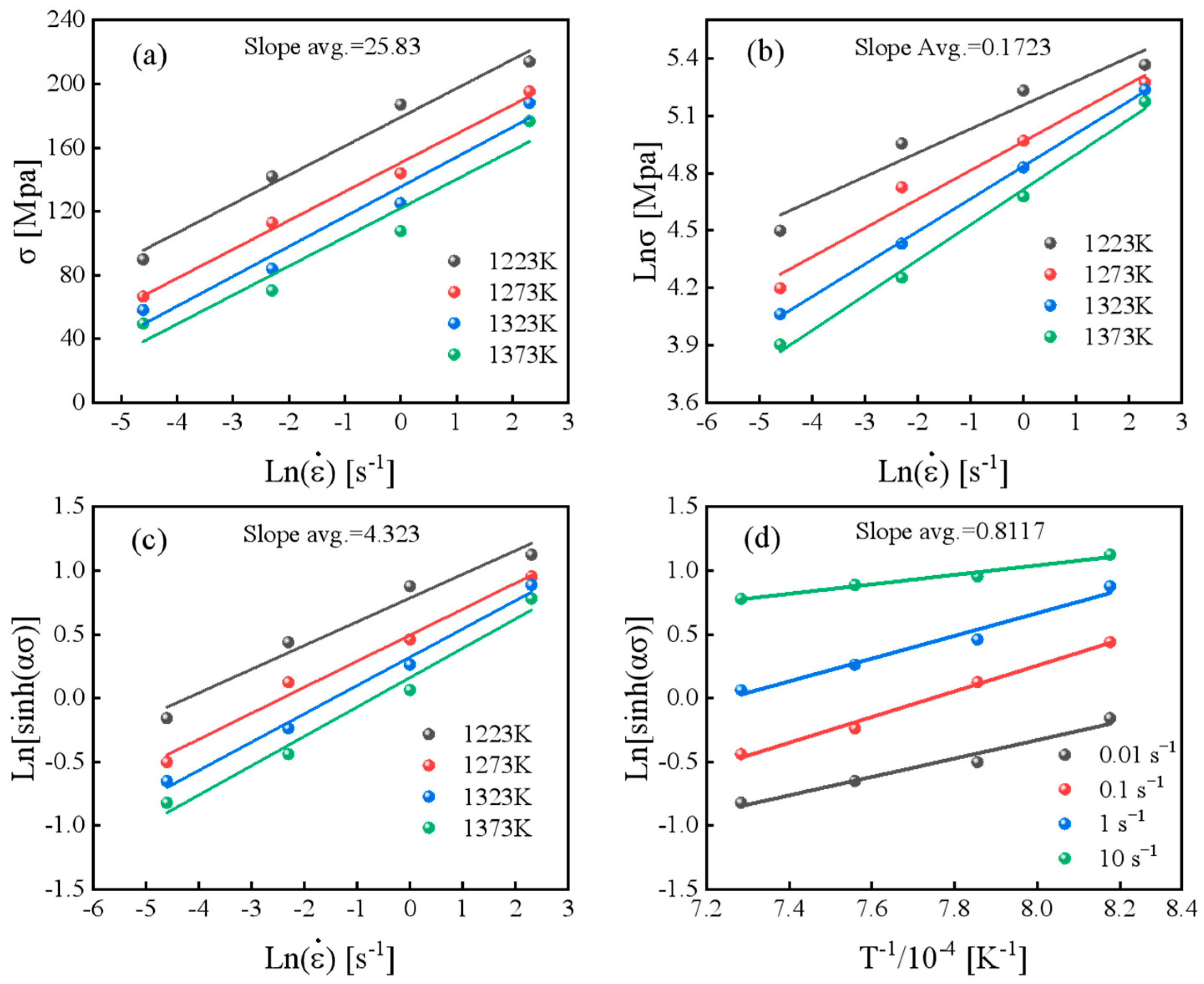
3.2.1. Arrhenius and Johnson–Cook Constitutive Model

The constitutive model of the Fe-Mn-Si-Cr-Ni alloy can be established by using the Zener–Hollomon parameter and the Arrhenius equations (Equations (1) and (2)). The final form of the Arrhenius model incorporating the Zener–Hollomon parameter is represented by Equation (3). The Zener–Hollomon parameter (Z) is introduced to quantify the combined effects of strain rate and temperature during high-temperature deformation. Its physical meaning lies in representing a temperature-compensated strain rate factor, which describes the influence of strain rate and temperature on the plastic deformation behavior of metals at elevated temperatures. During the development of the constitutive equations and the calculation of deformation activation energy, the Z parameter serves as a critical metric for evaluating the synergistic effects of strain rate and temperature in high-temperature deformation processes. At a high Z parameter (i.e., high strain rate and low temperature), the recrystallization process of alloys is primarily controlled by dynamic recovery (DRV), where dislocation slip becomes the dominant mechanism for plastic deformation. As the Z parameter decreases (e.g., at low strain rate or high temperature), DRX effect increases significantly, recrystallization volume fraction increases and grain boundary migration rate increases. At the same time, the synergistic effect of dislocation slip and grain boundary migration becomes the main driving force of the softening mechanism [31].

$$Z=\dot{\epsilon }\cdot \exp \left({\displaystyle \frac{Q}{R\cdot T}}\right)=F(\sigma )$$

(1)

$$\left\{\begin{array}{ll}\dot{\epsilon }=A\cdot \sinh {(\alpha \sigma )}^n\cdot \exp \left(-{\displaystyle \frac{Q}{R\cdot T}}\right)\hfill & (\mathrm{for}\mathrm{all}\sigma )\hfill \\ \dot{\epsilon }=A_1\cdot {\sigma }^{n1}\cdot \exp \left(-{\displaystyle \frac{Q}{R\cdot T}}\right)\hfill & (\alpha \sigma <0.8)\hfill \\ \dot{\epsilon }=A_2\cdot \exp (\beta \sigma )\cdot \exp \left(-{\displaystyle \frac{Q}{R\cdot T}}\right)\hfill & (\alpha \sigma >1.2)\hfill \end{array}\right.$$

(2)

$$\sigma ={\displaystyle \frac{1}{\alpha }}\ln \left\{\left[{\left({\displaystyle \frac{Z}{A}}\right)}^{{\displaystyle \frac{1}{n}}}\right]+{\left[{\left({\displaystyle \frac{Z}{A}}\right)}^{{\displaystyle \frac{2}{n}}}+1\right]}^{{\displaystyle \frac{1}{2}}}\right\}$$

(3)

where $A$, n₁, n, α, β are material constants and satisfy α = β/n₁; $\dot{\epsilon }$ is strain rate (s⁻¹); R is gas constant, 8.314 J/(mol·K); T is absolute temperature (K); Q is hot deformation activation energy (kJ/mol); and σ is true stress (MPa).

The derivation of these material constants follows the methodology outlined in references [32,33], with the calculated parameters for specific strain levels presented in Figure 4. However, if the Zener–Hollomon–Arrhenius constitutive model is directly derived from Equation (3), significant fitting errors may arise. This discrepancy occurs because the conventional Arrhenius constitutive equations lack strain compensation terms, leading to substantial deviations between predicted stress values and experimental measurements during material thermal compression [34,35].

True strain exhibits complex nonlinear dependencies on these material constants. The constitutive model can be extended through two distinct approaches: (i) incorporating strain-dependent terms directly into the stress–strain relationship (Equation (4)), or (ii) expressing the original material constants as polynomial or exponential functions of strain. The latter approach introduces a higher number of fitting parameters compared to the former. This increased parameter dimensionality elevates both model complexity (due to nonlinear coupling terms) and uncertainty in parameter estimation. In order to study the calibration of multi-parameter complex models based on Bayesian inference, the second method is selected for correction.

$$\sigma =A{\sinh }^{-1}\left({\left({\displaystyle \frac{Z}{B}}\right)}^{{\displaystyle \frac{1}{n}}}\right)\cdot (1+D{ϵ}^{\mathrm{m}})$$

(4)

Therefore, it is necessary to first find all the material constants in the Arrhenius constitutive model under different strains, assuming that the material constants (α, n, Q, lnA) are polynomial functions of the true strain (Equation (5)), so that the strain is coupled to the constitutive model through these material constants (Equation (6)). Figure 5 shows the direct relationship between material constants and true strain.

$$W=C_0+C_1\cdot \epsilon +C_2\cdot {\epsilon }^2+C_3\cdot {\epsilon }^3+C_4\cdot {\epsilon }^4+C_5\cdot {\epsilon }^5+C_6\cdot {\epsilon }^6$$

(5)

where W is the material parameter or deformation activation energy; C₀, C₁, C₂, C₃, C₄, C₅, C₆ are coefficients; and $\epsilon$ is strain.

$$\left\{\begin{array}{l}\sigma ={\displaystyle \frac{1}{\alpha (\epsilon )}}\cdot \ln \left({\left({\displaystyle \frac{Z(\dot{\epsilon },\epsilon ,T)}{A}}\right)}^{{\displaystyle \frac{1}{n}}}+\sqrt{{\left({\displaystyle \frac{Z(\dot{\epsilon },\epsilon ,T)}{A}}\right)}^{{\displaystyle \frac{2}{n}}}+1}\right)\hfill \\ Z=\dot{\epsilon }\cdot \exp \left({\displaystyle \frac{Q}{R\cdot T}}\right)\hfill \\ \ln A(\epsilon )={\displaystyle \sum _{i=0}^k\ln A_i}\cdot {\epsilon }^i\hfill \\ n(\epsilon )={\displaystyle \sum _{i=0}^k{n}_i}\cdot {\epsilon }^i\hfill \\ Q(\epsilon )={\displaystyle \sum _{i=0}^m{Q}_i}\cdot {\epsilon }^i\hfill \\ \alpha (\epsilon )={\displaystyle \sum _{i=0}^m{\alpha }_i}\cdot {\epsilon }^i\hfill \end{array}\right.$$

(6)

A Zener–Hollomon–Arrhenius constitutive model of the Fe-Mn-Si-based alloy coupled with hot deformation strain is established by combining Equation (3). Comparison of experimental results and model predictions is shown in Figure 6. The parameters of the final model are as follows:

$$\left\{\begin{array}{l}\alpha =0.0109-0.0604\cdot \epsilon +0.3363\cdot {\epsilon }^2-0.9541\cdot {\epsilon }^3+1.508\cdot {\epsilon }^4-1.2452\cdot {\epsilon }^5+0.417\cdot {\epsilon }^6\hfill \\ n=5.277-15.69\cdot \epsilon +120.77\cdot {\epsilon }^2-498.84\cdot {\epsilon }^3+1003.90\cdot {\epsilon }^4-964.84\cdot {\epsilon }^5+357.21\cdot {\epsilon }^6\hfill \\ Q=316.78-706\cdot \epsilon +6901\cdot {\epsilon }^2-\mathrm{29,759}\cdot {\epsilon }^3+\mathrm{59,547}\cdot {\epsilon }^4-\mathrm{56,680}\cdot {\epsilon }^5+\mathrm{20,835}\cdot {\epsilon }^6\hfill \\ \ln A=27.11-60.07\cdot \epsilon +611.12\cdot {\epsilon }^2-2688.37\cdot {\epsilon }^3+5436.94\cdot {\epsilon }^4-5208.98\cdot {\epsilon }^5+1922.70\cdot {\epsilon }^6\hfill \end{array}\right.$$

(7)

The Johnson–Cook (J-C) model, an empirical constitutive framework initially proposed in 1983 [36], describes the high-temperature deformation behavior of metallic alloys by explicitly incorporating strain rate sensitivity. The specimens were tested uniaxially to determine the different material properties required for the J-C model, which consists of five parameters, including A, B, C, n, and m [12,37]. The core idea is to couple the strain hardening term, strain rate effect term and temperature softening term by product form, and the expression is as follows:

$$\sigma =(A+B{\epsilon }^n)(1+C\ln {\dot{\epsilon }}^{\ast })(1-T^{\ast m})$$

(8)

where A is the initial yield stress (MPa) at the reference strain rate and temperature; B is the strain hardening coefficient (MPa); n is the strain hardening exponent; C is the strain rate sensitivity coefficient; and m is the temperature softening exponent.

$$\sigma =A+B{\epsilon }^n$$

(9)

The parameter calibration method refers to References [38,39]. The model takes into account the strain hardening, strain rate hardening, and thermal softening effects during deformation. While its multiplicative formulation (Equation (8)) provides computational simplicity, this decoupled treatment of mechanisms introduces inherent limitations. Neglecting temperature and strain rate, a nonlinear fit using the origin gives B as 236.63 and n as 0.0023. When the strain rate is 10 s⁻¹, the value of n is too small to be obtained by the origin fitting tool and can only be obtained by mathematical deduction (Equation (9)). As can be seen from Equation (8) above, the traditional Johnson–Cook constitutive model takes into account the hardening effect induced by strain and strain rate, as well as the softening effect caused by temperature T. These effects are combined through multiplication, without considering the interaction among them. This makes the model inaccurate under high-temperature conditions of the predetermined value, and the error is large, indicating that the model lacks a certain degree of accuracy. For this reason, based on the original model, considering the coupling effect between their three effects, the J-C prediction model (Equation (10)) modified from the original model is used to solve the process reference [40].

$$\sigma =(A_1+B_1\epsilon +B_2{\epsilon }^2)\left(1+C\ln {\displaystyle \frac{\dot{\epsilon }}{{\dot{\epsilon }}_{\mathrm{ref}}}}\right)\exp \left[\left(Q(\epsilon )+V(\dot{\epsilon },\epsilon )\ln {\displaystyle \frac{\dot{\epsilon }}{{\dot{\epsilon }}_{\mathrm{ref}}}}\right)(T-T_{\mathrm{ref}})\right]$$

(10)

A comparison between experimental results and model predictions is presented in Figure 6. The mean relative errors between predicted values and experimental values of Arrhenius model and J-C model were 4.56% and 5.85%, respectively. In terms of prediction accuracy, the Arrhenius model exhibits slightly higher accuracy than the J-C model, though both effectively predict flow behavior. However, as indicated by the red highlighted area in Figure 6, the Arrhenius model outperforms the J-C model in predicting flow behavior when a pronounced softening effect is present. Therefore, the Arrhenius model is more suitable for predicting the behavior of Fe-Mn-Cr alloys with a significant softening effect during hot deformation, while the J-C model is better suited for materials exhibiting a weak softening effect during hot deformation or for cold deformation scenarios.

3.2.2. Constitutive Model Fitting Based on Numerical Optimization

The solution process of the two constitutive models mentioned above is obtained by traditional mathematical deduction, and the solution process is complex. The numerical optimization method not only directly handles the Arrhenius model with coupled strain and the J-C model with high nonlinearity, but also does not need to linearize or simplify the model. It also enables the simultaneous optimization of multiple coupled parameters, such as strain hardening terms, strain rate terms, and temperature terms. The Arrhenius model and J-C model are numerically optimized by using MATLAB’s fminsearch function, and the effects of different initial guess model parameters and interpolation strain point ranges on fitting results are compared. The software version used in this study is MATLAB R2022a. The parallel computing functionality in MATLAB is utilized to accelerate the evaluation of the objective function. Three kinds of J-C models with different strain point ranges were designed: A: [0.05:0.05:0.8]; B: [0.05:0.02:0.8]; C: [0.1:0.02:0.8]; additionally, an Arrhenius model with initial parameters set to 1 was designed as variant D.

Figure 7 shows that when the number of parameters is large and the amount of data is large, the optimization process takes a long time and it is easy to fall into local optimization. Comparing the corresponding parameters of

Table 2. Parameters of the Arrhenius model based on numerical optimization fitting: the initial parameters are all set to 1.

Parameters	1	2	3	4	5	6
A	−0.0569	1.1087	0.7647	0.1072	1.1580	0.9807
n	1.0579	1.783	2.823	1.314	1.091	1.715
Q	0.84578	0.176	1.266	1.249	0.795	1.261
α	0.083725	−0.51288	0.59375	0.55653	1.0432	1.0745

and Equation (7), an improper initial guess may lead to optimization failure, and the optimization result may violate the physical meaning of the parameters, requiring additional constraints or relying on experience for multiple attempts. To sum up, although the method of fitting a constitutive model through numerical optimization can improve the calculation efficiency and prediction accuracy, the fitted parameters may violate the physical meaning of the parameters and require adjustment of the parameter range many times, and this method does not reduce the workload.

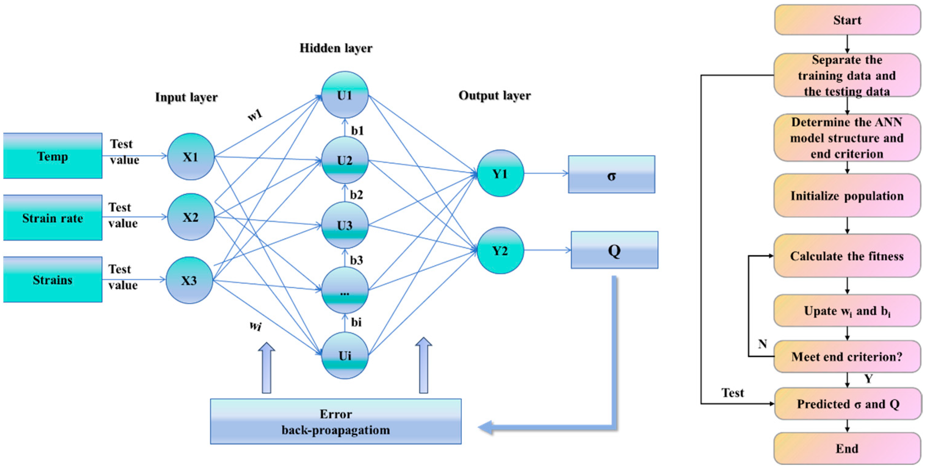
3.3. Establishment and Optimization of ANN Model

3.3.1. ANN Model

The back-propagation artificial neural network (BP-ANN) represents a foundational machine learning algorithm that enables computational systems to acquire learning capabilities through error gradient propagation [41,42,43]. Leveraging the enhanced nonlinear mapping capabilities of neural networks, flow stress modeling achieves 40% reduction in development time compared to conventional regression approaches. However, BP-ANN also has limitations. As the number of layers and neurons increases, the BP-ANN structure may become overly complex. This means that the model’s complexity increases and may include many unnecessary connections and neurons. And overfitting is also a significant drawback of BP-ANN. Due to the strong fitting ability of neural networks, it may overlearn details and noise in training data, while ignoring general rules of the data [17]. The input layer, hidden layer, and output layer are the three basic components of BP-ANN (Figure 8). In this study, the input layer consists of three neurons corresponding to the three deformation parameters of temperature, strain rate, and strain, while the output layer consists of neurons containing flow stress [44]. Written using MATLAB, this study builds the BP-ANN model by providing 257 experimental datasets, a relatively small number compared to other analyses performed using ANN models. The activation function from the input layer to the hidden layer is the tansig function, while the activation function from the hidden layer to the output layer is the purelin linear activation function, and the hidden layer contains 10 neurons. The maximum number of training iterations is set to 1000, the maximum number of validation failures is 10, and the target error is 1 × 10⁻⁷.

3.3.2. Structure Optimization of ANN Model

The architecture of artificial neural networks (ANNs) comprises three critical components: (1) activation functions, (2) number of hidden layers, and (3) neuron count per layer. Treating these three components as variables, we search for the optimal ANN model structure.

Firstly, ANN models with different activation functions are trained by fixing the number of hidden layers and the number of neurons. In this study, we used different activation functions, such as the tansig function (Equation (11)) from the input layer to the hidden layer and the purelin linear (Equation (12)) activation function from the hidden layer to the output layer. As shown in Figure 9a, it is obvious that the three activation functions from the input layer to the hidden layer have little effect on the ANN performance, while the linear activation function from the hidden layer to the output layer has better performance than the other two. Subsequently, ANN models with fixed activation function and assuming equal number of neurons at each time are trained with different hidden layer layers and numbers of neurons. As shown in Figure 9b, when the number of neurons is 12–16, optimal balance is provided.

$$f(x)={\displaystyle \frac{2}{1+e^{-2x}}}-1$$

(11)

$$f(x)=\mathrm{x}$$

(12)

Too few neurons may lead to underfitting, failing to capture complex rheological behavior. Too many neurons may result in overfitting and diminish the model’s generalization ability. Computational complexity scaled exponentially with hidden layers. Single-hidden-layer architectures demonstrated 2.1 times faster convergence while maintaining accuracy. Fewer hidden layers can only capture the basic temperature–strain-rate relationship, failing to represent nonlinear effects like strain hardening and dynamic recrystallization. In this study, we have not developed a Microscopic Mechanism Model, so an ANN model with a single hidden layer can effectively predict the results. From the perspective of the principles of neural networks, the role of the hidden layers is to learn the features and patterns of the input data. For models that incorporate microscopic mechanisms or involve cross-scales, since they involve multiple scales and complex physical processes, more hidden layers are required to learn these intricate features and patterns. Therefore, when it is necessary to construct such models, a single hidden layer cannot meet the computational requirements, and the number of hidden layers needs to be further discussed.

The activation function is categorized into two types: the activation function from the input layer to the hidden layer and the activation function from the hidden layer to the output layer. The number of neurons can also vary at each instance. If the activation function, the number of hidden layers and the number of neurons in each hidden layer are considered simultaneously, the dataset of ANN model structure parameters becomes very large. Employing a single manual search to compare and identify the best structure demands significant computational effort. Therefore, improving the optimization speed of the ANN model structure and reducing the iteration time are crucial. In addition to manual search and random sample search, Bayesian optimization can also be utilized for optimization. For small-scale datasets, Bayesian algorithms have fewer iterations and are faster than other tuning methods. Therefore, Bayesian optimization is used to find the optimal ANN model structure. The ANN model is coded by MATLAB, the Bayesian optimization algorithm is called by MATLAB’s toolbox, and parallel calculation is used for training. Compared with grid search, the efficiency of this method is improved by about 5-8 times, and better network configuration can be observed. It is found that a single-hidden-layer network composed of 12 neurons has the optimal configuration for the current problem.

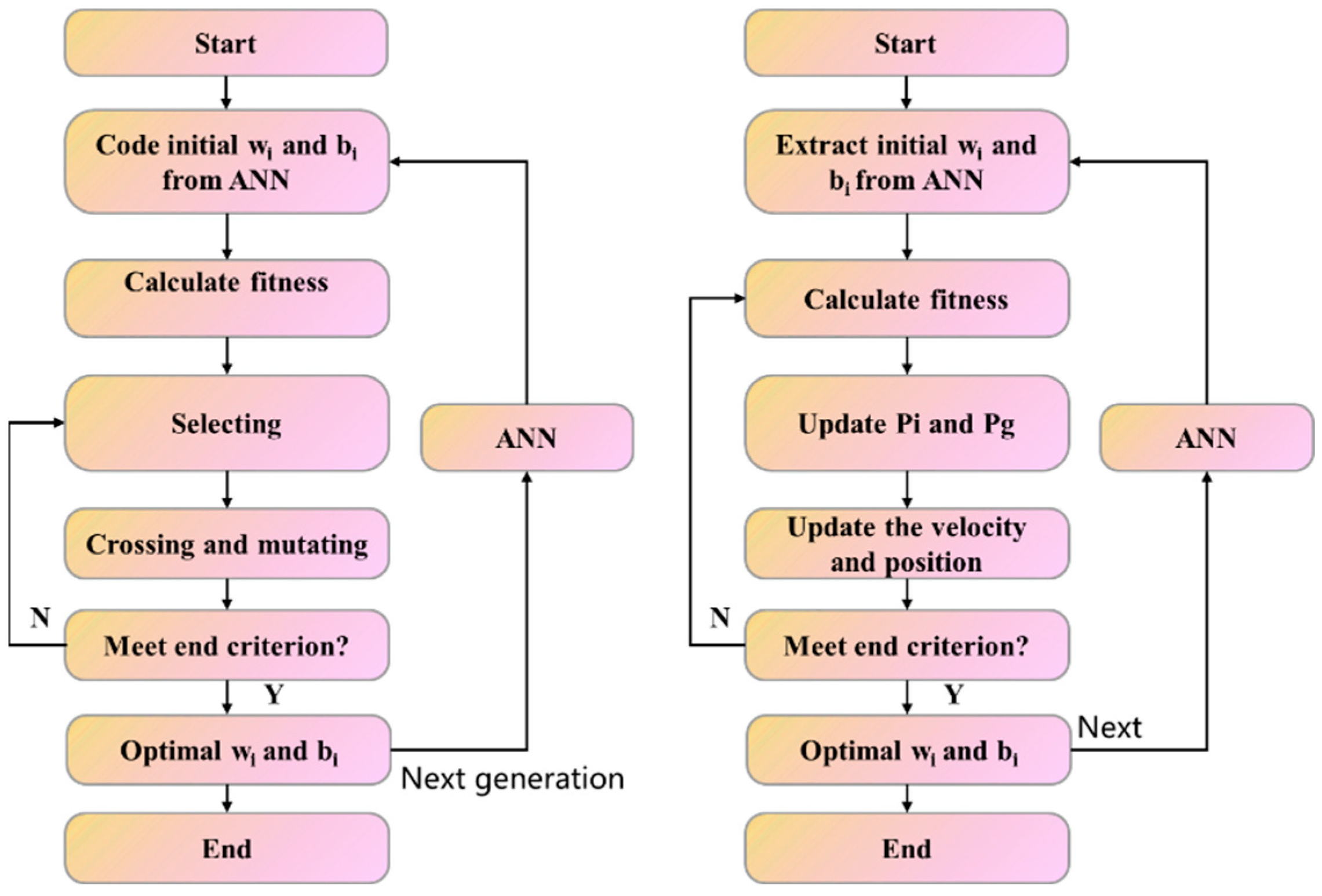
3.3.3. Optimization Algorithm

The structure of traditional back-propagation artificial neural network (BP-ANN) models is influenced not only by hyperparameters but also by weights and biases, which affect prediction accuracy and can lead to overfitting. Fortunately, intelligent optimization algorithms can solve these problems by optimizing weights, biases, and hyperparameters. For example, BP-ANN models can be enhanced using genetic algorithms (GAs), particle swarm optimization (PSO) algorithms, or hybrid algorithms. In this study, the weights and biases are optimized using GA and PSO algorithms. The GA-BP network optimizes the initial weights and biases of the network using a genetic algorithm, which explores a larger solution space through natural selection, crossover, and mutation, before further refining the weights and biases with the back-propagation algorithm. The PSO algorithm simulates the foraging behavior of birds, with its particles representing combinations of weights and biases in the BP neural network. These particles move within the solution space, dynamically adjusting their speed and position based on their own experience and the group’s optimal position, before being locally optimized and adjusted by the back-propagation algorithm of the BP neural network. Using the MATLAB toolbox to call two optimization algorithms, Figure 10 presents a comparison of model prediction results after optimizing weights and biases with different optimization algorithms. Figure 11 compares the prediction capabilities of the Arrhenius model, BP-ANN model, GA-BP-ANN model, and PSO-BP-ANN model, all coupled with strain, under the same number of strain data points as input. From Figure 12, it can be seen that the R and AARE values of the Arrhenius model coupled with strain are 0.9934 and 4.56%. The R and AARE values for the BP-ANN model, GA-BP-ANN model, and PSO-BP-ANN model are 0.9979, 0.9985, and 0.9982, and 3.6%, 3.01%, and 3.18%, respectively. It is evident that data fitting through machine learning offers higher prediction accuracy than traditional mathematical derivation models, while also significantly improving computational efficiency and reducing workload. Prediction accuracy can be further enhanced by using optimization algorithms, though the difference between the two optimization algorithms is not significant. However, the parameters obtained from such optimization algorithms still exhibit uncertainty, and the generalization ability of the model remains limited. Therefore, quantifying the hyperparameters of the ANN is crucial.

4. Discussion

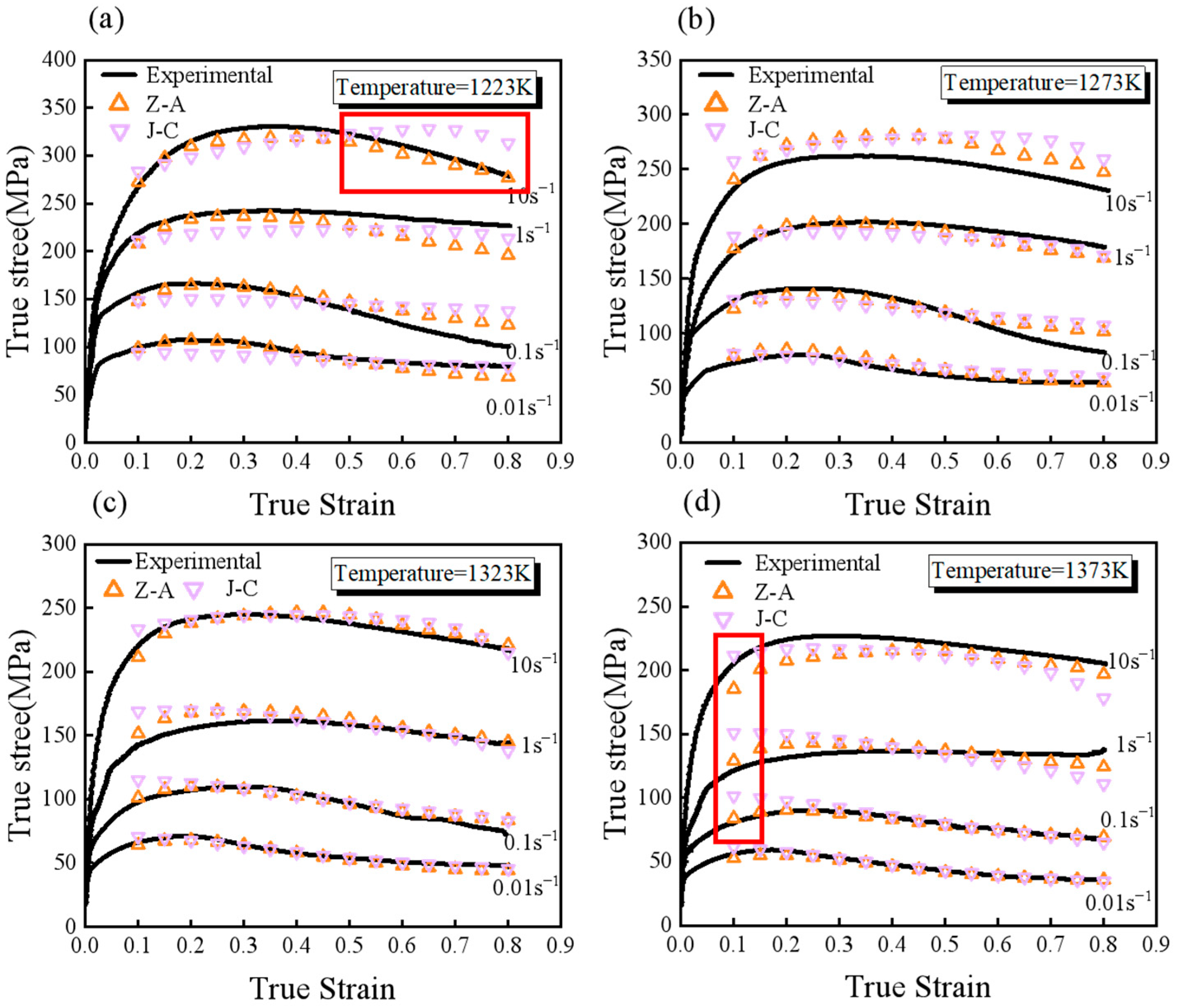
4.1. Mathematical Derivation vs. Numerical Optimization vs. Machine Learning

In the selection of material constitutive modeling methods, traditional mathematical deduction fitting, traditional optimization methods, and machine learning methods exhibit significant differences, which arise from fundamental distinctions in modeling theory and technical approaches (

Table 3. Comparison of the advantages and disadvantages of the three methods.

Characteristics	Mathematical Derivation	Numerical Optimization	Machine Learning Method
Model Structure	Explicit physical equations	Explicit equations and parameter optimization	Blac-box model
Data Requirements	Low	Medium	High
Computational Efficiency	High	Medium	Low
Interpretability	Strong	Medium	Weak
Complex Nonlinear Model	Weak	Medium	Strong
Generalization Ability	Low	Medium	High
Applicable Scenarios	Simple behavior verification, theoretical derivation	Multi-parameter coupling optimization	Complex multi-field coupling, big data scenarios

).

Traditional mathematically derived fits are based on explicit physical equations (e.g., power laws or exponential forms) and rely on rigorous theoretical assumptions for modeling. The advantages of this method are its use of few parameters, strong interpretability (as parameters have clear physical meanings), and its ability to validate the model’s effectiveness with a small amount of experimental data without requiring large datasets. However, its model structure is constrained by the preset equations form, making it difficult to characterize complex nonlinear relationships, and its generalization ability depends on the universality of the physical assumptions. For example, the J-C constitutive model in Section 3.3.2 can also predict the flow behavior of hot compression at high temperatures, but when the softening effect of the material is obvious, the model fitting effect will be reduced. Similarly, when describing hyperelastic materials, Mooney–Rivlin models simplify calculations with two parameters but fail to capture multiscale coupling effects [45].

Traditional optimization methods retain an explicit equations framework and adjust model parameters by optimization algorithms (such as genetic algorithm and gradient descent), so as to improve the fitting accuracy of experimental data. Compared with pure mathematical derivation, this method allows flexible optimization of parameters within physical constraints and can deal with polynomial nonlinear terms, but the optimization process may deviate parameters from their original physical meanings. The data need to cover the sensitive region of parameters, the computational efficiency is limited by the convergence speed of the optimization algorithm, and regularization techniques are usually needed to avoid the risk of overfitting. For example, the numerical optimization fitting constitutive model in Section 3.3.3 can predict the flow behavior quickly, but the fitting constitutive model parameters deviate severely from the physical meaning. Moreover, the initial guesses for model parameters, as well as the range and number of fitted data points, influence the results of numerical optimization.

The machine learning method adopts a black-box model structure, enabling it to approximate arbitrary nonlinear relationships without an explicit equation through extensive data-driven training. Its core advantage lies in its ability to handle multi-field coupling, complex material behavior, and other systems that are challenging for traditional models to describe, with generalization ability significantly surpassing that of traditional methods when data quality is high. However, this method faces high computational costs, weak interpretability, and overfitting risks. For example, deep neural networks can achieve more than 95% accuracy in composite damage prediction, but they require a large amount of demonstration data to train models, and physical mechanisms are difficult to trace. For instance, Section 3.3.2 optimizes weights and biases using different optimization algorithms, while Section 3.3.3 optimizes structures to significantly enhance prediction accuracy, reduce computational efficiency, and lower computational costs. However, the number of weight parameters far exceeds that of physical parameters, introducing risks of overfitting, weak interpretability, and uncertain extensibility.

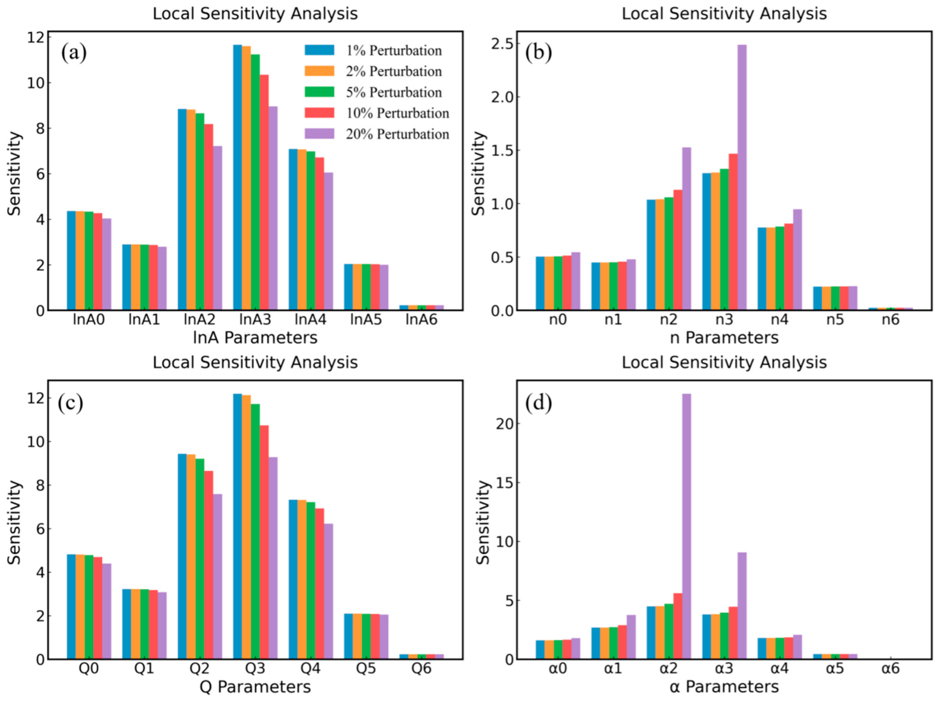
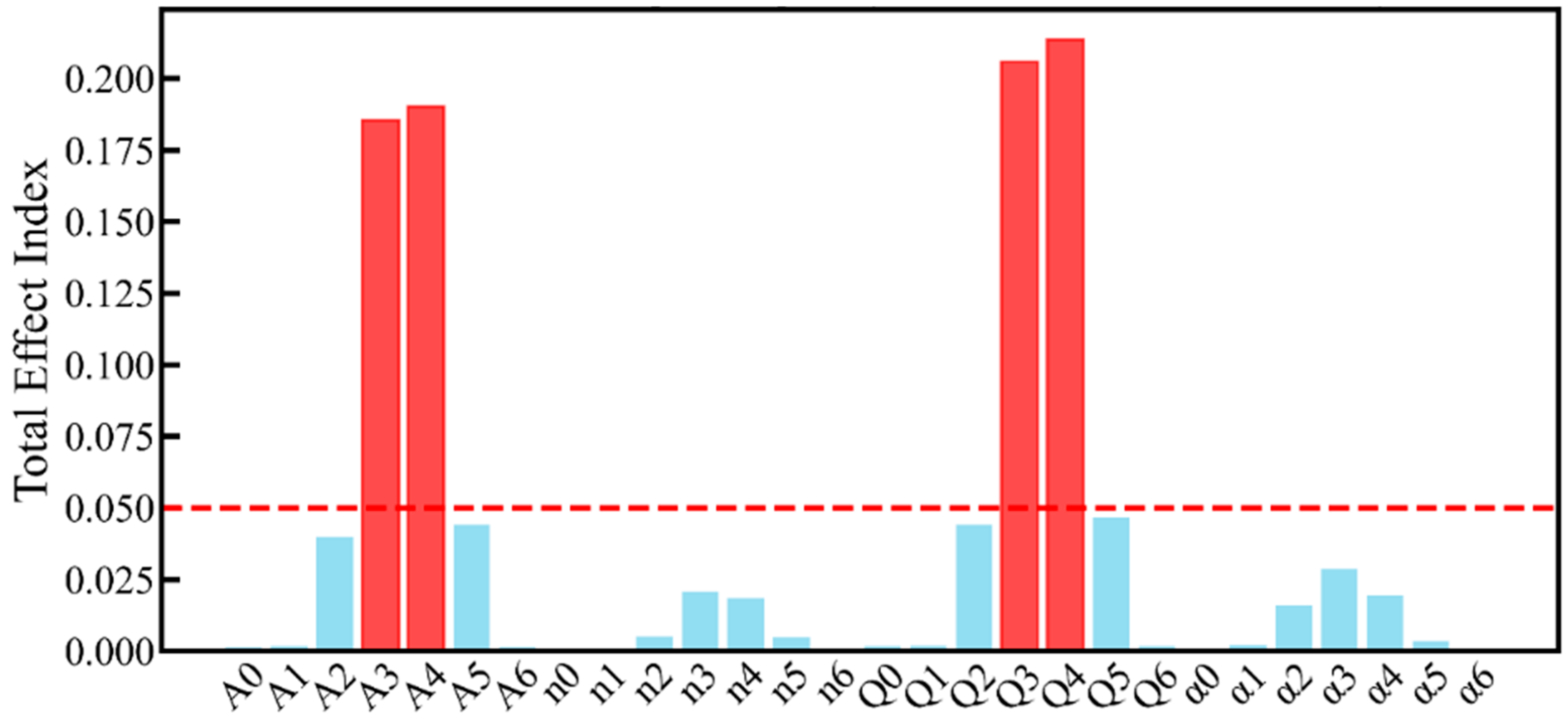
4.2. Sensitivity Analysis of Constitutive Model Parameters

Bayesian optimization is a global optimization method based on Bayes’ theorem, which is used to find the optimal solution of the objective function in a high-dimensional space. Its basic steps are as follows: First, build a surrogate model, using a probabilistic model like the Gaussian process to estimate the posterior distribution of the objective function. Then, define an acquisition function, such as Expected Improvement, to measure the value of evaluating at a certain point. Next, select the next evaluation point by maximizing the acquisition function. After that, evaluate the objective function at the new evaluation point and update the parameters of the surrogate model. Repeat the steps of selecting evaluation points and updating the model until the stopping condition is met, such as reaching the maximum number of evaluations or the improvement of the objective function being less than a certain threshold.

For modified Arrhenius model and Johnson–Cook model coupled with strain, direct parameter calibration by numerical optimization increases the calculation cost and the parameters cannot be specifically calibrated. To identify parameters that significantly affect prediction accuracy and the underlying physical mechanisms, sensitivity analysis is employed to determine which parameters exert a substantial influence on model output. For example, in the Johnson–Cook model, strain-hardening and heat-softening parameters greatly influence the accuracy of simulation results [46]. This identification process helps to concentrate resources and improve efficiency in parameter optimization. Parameter sensitivity analysis methods include local sensitivity analysis (LSA) and global sensitivity analysis (GSA). Local sensitivity estimates sensitivity coefficients by making small perturbations to each input parameter. The sensitivity coefficient is calculated as shown in Equation (11). Figure 13 presents the results of local sensitivity analysis for the 24 parameters of the Arrhenius constitutive model, as solved in Section 3.2.1. The sensitivity coefficient is derived by sampling at a 10% increase or decrease from a known parameter value, using the Latin Hypercube Sampling (LHS) method and applying Equation (13). The sensitivity coefficients of Figure 13a and c are generally too high for subsequent parameter evaluation based on the results of local sensitivity analysis. The advantage of local sensitivity analysis is that it is computationally efficient and suitable for rapid screening in high-dimensional parameter spaces, but it only reflects the first-order influence of parameters in local neighborhoods, ignoring interaction effects and global nonlinear responses. While it is well suited for linear or nearly linear models, its effectiveness diminishes for nonlinear problems.

$$S_i={\displaystyle \frac{\partial \sigma }{\partial p_i}}\approx {\displaystyle \frac{\sigma (p_i+\Delta )-\sigma (p_i-\Delta )}{2\Delta }}$$

(13)

Local sensitivity analysis differs from global sensitivity analysis. Local sensitivity analysis considers only small perturbations of parameters near a specific point, typically employing derivative or finite difference methods, and is deterministic in nature. Global sensitivity analysis examines the variation of parameters across their entire possible range, often using random methods such as Monte Carlo sampling, which may yield slight variations in results (though these can be stabilized by setting random seeds). Unlike local sensitivity analysis, global sensitivity analysis evaluates the full range of input parameters and quantifies their impact on model outputs by assessing interactions between parameters [47]. The Sobol index method, Morris screening method, and regression analysis are commonly employed in global sensitivity analysis. The advantage of global sensitivity analysis lies in its ability to capture complex nonlinear and interactive effects, making it more suitable for complex engineering problems than local sensitivity analysis. However, it is computationally intensive, particularly in high-dimensional parameter spaces, where large amounts of sample data may be required. In the Sobol method, the output variance can be decomposed into the sum of the main effects and interaction effects of each input parameter (Equation (14)).

$$\mathrm{Var}(Y)={\displaystyle \sum _{i=1}^p{V}_i}+{\displaystyle \sum _{i<j}{V}_{ij}}+\cdots +V_{12\cdots p}$$

(14)

$$S_{T_i}={\displaystyle \frac{E_{X_{~i}}[{\mathrm{Var}}_{X_i}(Y|X_{~i})]}{\mathrm{Var}(Y)}}$$

(15)

To further evaluate the interactions between parameters, a global sensitivity analysis of 24 parameters of the Arrhenius constitutive model was performed using the Sobol method. Through local sensitivity analysis, it was found that when most parameters are perturbed by 1% or more, the prediction results change significantly; thus, a ±1% perturbation is used for global sensitivity screening, and the global sensitivity index of the parameters is calculated in combination with Equation (15). An S_T value greater than 1 is considered to be highly sensitive, and the parameters have a decisive influence on the output, usually directly related to the core physical mechanism. When S_T is between 0.05 and 1, it is considered to be moderately sensitive, and parameters have significant influence on output but are not dominant factors. An ST value less than 0.05 is considered as low sensitivity, and parameter influence can be ignored. Combining Figure 13 and Figure 14, it is obvious that the sensitivity index of A3, A4, Q3, and Q4 is much higher than that of other parameters, and these four parameters are regarded as sensitive parameters (

Table 4. Sensitivity parameters and sensitive intervals obtained from global sensitivity analysis.

Rank	Parameter	Sensitivity	Range (Min: Max)
1	Q3	0.2099	[−30,057.26: 29,462.06]
2	Q4	0.2096	[58,952.18: 60,143.14]
3	A4	0.1929	[5382.57: 5491.31]
4	A3	0.1922	[−2715.25: −2661.49]

).

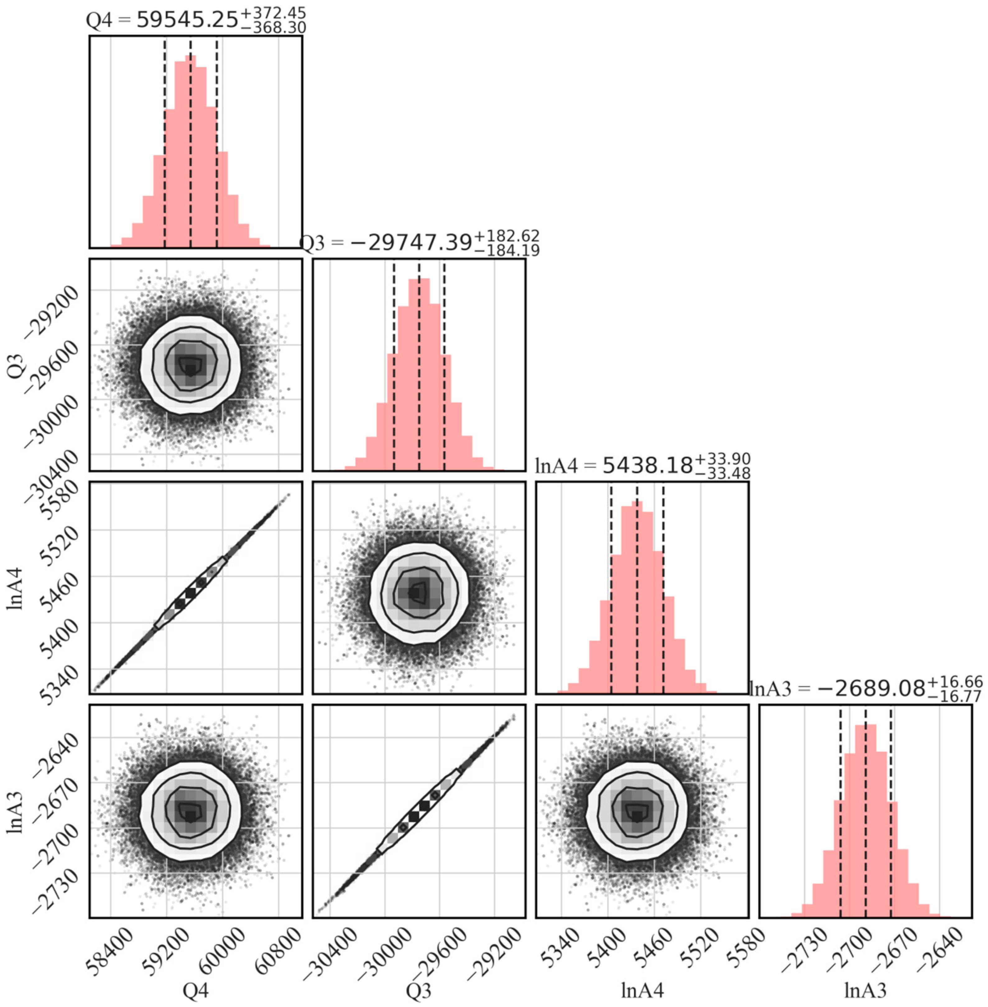
4.3. Parameter Evaluation and Calibration Based on Bayesian Reasoning

Bayesian posterior probability density calibration parameters are used to construct likelihood function (Equations (16) and (17)). In this study, a Gaussian Process Regression (GPR) proxy model is used to predict the mean and standard deviation of output values [48]. The prediction error is assumed to be normally distributed, where $\mu (\theta )$ is the mean of the GPR prediction (i.e., proxy model output); $\sigma (\theta )$ is the standard deviation of the GPR prediction (quantifies model uncertainty); and $y$ is the actual observed value, where the residual between the observed value and the predicted mean is assumed to be 0.

$$p(D|\theta )=N(y|\mu (\theta ),{\sigma }^2(\theta ))$$

(16)

$$p(D|\theta )={\displaystyle \frac{1}{\sqrt{2\pi }{\sigma }_{\mathrm{error}}}}\exp \left(-{\displaystyle \frac{{({\sigma }_{\exp }-{\sigma }_{\mathrm{model}}(\theta ))}^2}{2{\sigma }_{\mathrm{error}}^2}}\right)$$

(17)

Then, the prior probability (Equation (18)) is determined, and uniform distribution prior adopted, that is, the parameters are equally distributed in the defined interval. d is the parameter dimension.

$$p(\theta )=\left\{\begin{array}{ll}{\displaystyle \prod _{i=1}^d\frac{1}{{\theta }_i^{\max }-{\theta }_i^{\min }}}\hfill & \left(\mathrm{if}{\theta }_i\in [{\theta }_i^{\min },{\theta }_i^{\max }], \forall i\right)\hfill \\ 0\hfill & \left(\mathrm{otherwise}\right)\hfill \end{array}\right.$$

(18)

Finally, the marginal likelihood function is solved. Because it is extremely difficult to calculate this integral directly (Equation (19)) in a high-dimensional parameter space, the Markov Chain Monte Carlo (MCMC) method directly approximates the posterior distribution (Equation (20)) by generating samples that obey the posterior distribution [49]. During the sampling process, the mixing efficiency of the chain is ensured by adjusting the adaptive step size, and finally, the posterior mean and confidence interval of the parameters are calculated based on the converged samples. This method quantifies parameter uncertainty effectively and avoids the local optimization trap. This study uses emcee, a powerful and widely used Python library for Markov Chain Monte Carlo (MCMC) sampling, to implement this part of the computation. The version of Python used in this study is 3.12.

$$p(D)={\displaystyle {\int }_{\theta }p}(D|\theta )p(\theta )d\theta$$

(19)

$$p(\theta |D)\propto p(D|\theta )p(\theta )$$

(20)

The posterior distributions of sensitive parameters were obtained by Bayesian calibration of model parameters using the Markov Chain Monte Carlo (MCMC) method [50]. A corner plot was generated using python to show the posterior distribution of parameter space and the correlations between parameters. Figure 15 consists of several subplots, where each subplot on the diagonal represents the marginal distribution of one parameter and the scatterplot on the off-diagonal represents the joint distribution of two parameters. It follows that Q3 and Q4 have strong correlations with lnA3 and lnA4, respectively, and other parameter combinations have weak correlations. Confidence intervals for the four parameters and calibration parameters are shown in Figure 15. The correlation coefficient (R²) between the predicted stress–strain curve and the experimental data is 0.983, which is significantly higher than the original parameter (R² = 0.942).

Bayesian posterior probability density analysis can not only improve the calibration accuracy of parameters but also reveal the physical meaning and uncertainty associated with those parameters. The key parameters of the constitutive equation for thermal deformation are calibrated and analyzed using Bayesian inference. The difference in confidence interval width of each parameter indicates that the sensitivity of the model to different deformation conditions is different, and the uncertainty of parameters in the low-temperature and high-strain region is relatively high, which is consistent with the possibility of complex dynamic recrystallization and dynamic recovery mechanism in this region. Covariance matrix analysis revealed significant correlation between the activation energy and frequency factor, indicating that these parameters are coupled in describing the thermal activation deformation process, which is consistent with the thermal deformation theory. The residual analysis by substituting calibrated parameters into the model shows that the prediction deviation of the model is large in the medium strain region (ε = 0.2–0.4), which may be related to the dynamic softening mechanism occurring in this stage. It is necessary to further improve the model by introducing additional microstructure evolution factors. Bayesian parameter calibration not only improves the prediction accuracy of the model, but also provides a new perspective for understanding the physical mechanism of hot deformation of Fe-Mn-Cr-based alloys.

Although this study mainly focuses on the thermomechanical constitutive modeling of Fe-Mn-Cr-based alloys, the data-driven methods used, such as artificial neural network models, Bayesian inference, and sensitivity analysis, have certain generality. The basic principles and technical means of these methods can be applied to the research on the thermomechanical behavior of other alloy systems. As long as there is sufficient experimental data, similar methods can be used for modeling and analysis. In future research, we will collect more thermomechanical experimental data of different alloy systems to further verify and expand the applicability of this method. It is possible to further explore the hybrid modeling method that combines traditional mathematical models and machine learning models, for example, by introducing microstructure information as input features into the machine learning model, or using the machine learning model to optimize the parameters of the mathematical model, so as to achieve a more accurate prediction of the deformation behavior of materials and a deeper understanding of the deformation mechanism.

5. Conclusions

In this study, the performance of traditional physical models and machine learning methods in modeling the rheological behavior of materials at high temperatures was systematically compared. Although different modeling methods have their own advantages, by reasonably integrating the explanatory ability of traditional physical models with the efficiency of modern calculation methods, the prediction accuracy of models can be significantly improved and the understanding of material deformation mechanism can be deepened. The main conclusions are as follows:

(1)

Traditional physical models (e.g., the Arrhenius model) offer physical interpretability in predicting high-temperature flow behavior but face challenges in parameter solving. Machine learning models (e.g., artificial neural networks), optimized via genetic algorithms, particle swarm optimization, and Bayesian optimization, achieve high-precision nonlinear modeling (R² = 0.9985, AARE = 3.01%). Numerical optimization, meanwhile, balances rapid parameter fitting with model interpretability. These three methodologies are, respectively, suited for distinct application scenarios: simplified physical modeling, complex nonlinear predictions, and efficient parameter optimization tasks.

(2)

The sensitivity analysis method is used to determine the key parameters (lnA3, lnA4, Q3, Q4) of the Arrhenius model which have the greatest influence on rheological behavior. Bayesian inference and MCMC sampling methods are used to quantify the uncertainty of model parameters and analyze the posterior probability density distribution of key parameters, so as to evaluate and calibrate parameters and improve the robustness of the model.

(3)

The Bayesian inference method significantly improves model accuracy, raising the correlation coefficient (R²) from 0.942 to 0.983 after parameter calibration. Posterior distribution analysis reveals key physical insights, including strong correlations between activation energy (Q3, Q4) and frequency factors (lnA3, lnA4), while identifying higher uncertainty in low-temperature and high-strain regions. This approach is valuable for both predicting Fe-Mn-Cr alloy deformation behavior and calibrating constitutive models of other metallic materials, with potential for integration with micromechanism modeling to enhance physical consistency and predictive accuracy.

References

- Khan, S.; Pydi, Y.S.; Mani Prabu, S.S.; Palani, I.A.; Singh, P. Development and Actuation Analysis of Shape Memory Alloy Reinforced Composite Fin for Aerodynamic Application. Sens. Actuators A Phys. 2021, 331, 113012. [Google Scholar] [CrossRef]
- Ghafoori, E.; Wang, B.; Andrawes, B. Shape Memory Alloys for Structural Engineering: An Editorial Overview of Research and Future Potentials. Eng. Struct. 2022, 273, 115138. [Google Scholar] [CrossRef]
- Algamal, A.; Abedi, H.; Gandhi, U.; Benafan, O.; Elahinia, M.; Qattawi, A. Manufacturing, Processing, Applications, and Advancements of Fe-Based Shape Memory Alloys. J. Alloys Compd. 2025, 1010, 177068. [Google Scholar] [CrossRef]
- Vilella, T.; Rodríguez, D.; Fargas, G. Additive Manufacturing of Ni-Free Ti-Based Shape Memory Alloys: A Review. Biomater. Adv. 2024, 158, 213774. [Google Scholar] [CrossRef] [PubMed]
- Pan, M.-M.; Zhang, X.-M.; Zhou, D.; Misra, R.D.K.; Chen, P. Fe–Mn–Si–Cr–Ni Based Shape Memory Alloy: Thermal and Stress-Induced Martensite. Mater. Sci. Eng. A 2020, 797, 140107. [Google Scholar] [CrossRef]
- Cladera, A.; Weber, B.; Leinenbach, C.; Czaderski, C.; Shahverdi, M.; Motavalli, M. Iron-Based Shape Memory Alloys for Civil Engineering Structures: An Overview. Constr. Build. Mater. 2014, 63, 281–293. [Google Scholar] [CrossRef]
- Sajadi, S.A.; Toroghinejad, M.R.; Rezaeian, A.; Ebrahimi, G.R. A Study of Hot Compression Behavior of an as-Cast Fecrcuni2mn2 High-Entropy Alloy. J. Alloys Compd. 2022, 896, 162732. [Google Scholar] [CrossRef]
- Deng, H.; Zheng, Z.; Song, W.; Tan, X.; Liang, X.; Li, H.; Li, H. Constitutive Model and Microstructure Evolution of Thermal Deformation Behavior of in Situ Tib2p/Al-Zn-Mg-Cu Composites with High Zn Content. Mater. Today Commun. 2024, 41, 110308. [Google Scholar] [CrossRef]
- Wang, M.; Zhang, G.; Hou, B.; Wang, W. Deep Learning Coupled Bayesian Inference Method for Measuring the Elastoplastic Properties of Ss400 Steel Welds by Nanoindentation Experiment. Measurement 2025, 242, 116092. [Google Scholar] [CrossRef]
- Zhang, Y.; Hart, J.D.; Needleman, A. Identification of Plastic Properties from Conical Indentation Using a Bayesian-Type Statistical Approach. J. Appl. Mech. 2019, 86, 011002. [Google Scholar] [CrossRef]
- Adarsh, S.H.; Sampath, V. Hot Deformation Behavior of Fe–28ni–17co-11.5al-2.5ta-0.05b (At.%) Shape Memory Alloy by Isothermal Compression. Intermetallics 2019, 115, 106632. [Google Scholar] [CrossRef]
- Rajoria, S.R.; Gulhane, S.; Khan Md, F.; Sahoo, B.N. Hot Deformation Behavior Study of Coarse Grained and Ultrafine Grained Qe22 Magnesium Alloy through Development of Constitutive Analysis and Johnson–Cook Model. J. Alloys Compd. 2025, 1013, 178530. [Google Scholar] [CrossRef]
- Portone, T.; Niederhaus, J.; Sanchez, J.; Swiler, L. Bayesian Model Selection for Metal Yield Models in High-Velocity Impact. Int. J. Impact Eng. 2020, 137, 103459. [Google Scholar] [CrossRef]
- Bernstein, J.; Schmidt, K.; Rivera, D.; Barton, N.; Florando, J.; Kupresanin, A. A Comparison of Material Flow Strength Models Using Bayesian Cross-Validation. Comput. Mater. Sci. 2019, 169, 109098. [Google Scholar] [CrossRef]
- Hamdia, K.M.; Zhuang, X.; He, P.; Rabczuk, T. Fracture Toughness of Polymeric Particle Nanocomposites: Evaluation of Models Performance Using Bayesian Method. Compos. Sci. Technol. 2016, 126, 122–129. [Google Scholar] [CrossRef]
- Ritto, T.G.; Nunes, L.C.S. Bayesian Model Selection of Hyperelastic Models for Simple and Pure Shear at Large Deformations. Comput. Struct. 2015, 156, 101–109. [Google Scholar] [CrossRef]
- Jeong, K.; Lee, K.; Lee, S.; Kang, S.-G.; Jung, J.; Lee, H.; Kwak, N.; Kwon, D.; Han, H.N. Deep Learning-Based Indentation Plastometry in Anisotropic Materials. Int. J. Plast. 2022, 157, 103403. [Google Scholar] [CrossRef]
- Shin, S.; Lee, Y.; Kim, M.; Park, J.; Lee, S.; Min, K. Deep Neural Network Model with Bayesian Hyperparameter Optimization for Prediction of Nox at Transient Conditions in a Diesel Engine. Eng. Appl. Artif. Intell. 2020, 94, 103761. [Google Scholar] [CrossRef]
- Jeong, K.; Lee, H.; Kwon, O.M.; Jung, J.; Kwon, D.; Han, H.N. Prediction of Uniaxial Tensile Flow Using Finite Element-Based Indentation and Optimized Artificial Neural Networks. Mater. Des. 2020, 196, 109104. [Google Scholar] [CrossRef]
- Rivera, D.; Bernstein, J.; Schmidt, K.; Muyskens, A.; Nelms, M.; Barton, N.; Kupresanin, A.; Florando, J. Bayesian Calibration of Strength Model Parameters from Taylor Impact Data. Comput. Mater. Sci. 2022, 210, 110999. [Google Scholar] [CrossRef]
- Madireddy, S.; Sista, B.; Vemaganti, K. A Bayesian Approach to Selecting Hyperelastic Constitutive Models of Soft Tissue. Comput. Methods Appl. Mech. Eng. 2015, 291, 102–122. [Google Scholar] [CrossRef]
- Papadimas, N.; Dodwell, T. A Hierarchical Bayesian Approach for Calibration of Stochastic Material Models. Data-Centric Eng. 2021, 2, e20. [Google Scholar] [CrossRef]
- Battalgazy, B.; Khatamsaz, D.; Ghasemi, Z.; Mallick, D.D.; Arroyave, R.; Srivastava, A. A Bayesian-Based Approach for Constitutive Model Selection and Calibration Using Diverse Material Responses. Acta Mater. 2025, 287, 120796. [Google Scholar] [CrossRef]
- Ryan, S.; Berk, J.; Rana, S.; McDonald, B.; Venkatesh, S. A Bayesian Optimisation Methodology for the Inverse Derivation of Viscoplasticity Model Constants in High Strain-Rate Simulations. Def. Technol. 2022, 18, 1563–1577. [Google Scholar] [CrossRef]
- Aggarwal, A.; Hudson, L.T.; Laurence, D.W.; Lee, C.-H.; Pant, S. A Bayesian Constitutive Model Selection Framework for Biaxial Mechanical Testing of Planar Soft Tissues: Application to Porcine Aortic Valves. J. Mech. Behav. Biomed. Mater. 2023, 138, 105657. [Google Scholar] [CrossRef]
- Haj-Ali, R.; Kim, H.-K.; Koh, S.W.; Saxena, A.; Tummala, R. Nonlinear Constitutive Models from Nanoindentation Tests Using Artificial Neural Networks. Int. J. Plast. 2008, 24, 371–396. [Google Scholar] [CrossRef]
- Ji, H.; Duan, H.; Li, Y.; Li, W.; Huang, X.; Pei, W.; Lu, Y. Optimization the Working Parameters of as-Forged 42crmo Steel by Constitutive Equation-Dynamic Recrystallization Equation and Processing Maps. J. Mater. Res. Technol. 2020, 9, 7210–7224. [Google Scholar] [CrossRef]
- Li, D.Z.; Zhao, X.M.; Zhang, H.L.; Li, J. Flow Stress-Strain Curves and Dynamic Recrystallization Behavior of High Carbon Low Alloy Steels during Hot Deformation. J. Mater. Res. Technol. 2025, 35, 3144–3160. [Google Scholar] [CrossRef]
- He, X.; Liu, L.; Zeng, T.; Yao, Y. Micromechanical Modeling of Work Hardening for Coupling Microstructure Evolution, Dynamic Recovery and Recrystallization: Application to High Entropy Alloys. Int. J. Mech. Sci. 2020, 177, 105567. [Google Scholar] [CrossRef]
- Li, C.; Huang, L.; Zhao, M.; Zhang, X.; Li, J.; Li, P. Influence of Hot Deformation on Dynamic Recrystallization Behavior of 300m Steel: Rules and Modeling. Mater. Sci. Eng. A 2020, 797, 139925. [Google Scholar] [CrossRef]
- He, J.; Hu, M.; Zhou, Z.; Li, C.; Sun, Y.; Zhu, X. Effect of Initial Grain Size on Hot Deformation Behavior and Recrystallization Mechanism of Al-Zn-Mg-Cu Alloy. Mater. Charact. 2024, 212, 114012. [Google Scholar] [CrossRef]
- Karimzadeh, M.; Malekan, M.; Mirzadeh, H.; Saini, N.; Li, L. Hot Deformation Behavior Analysis of as-Cast Cocrfeni High Entropy Alloy Using Arrhenius-Type and Artificial Neural Network Models. Intermetallics 2024, 168, 108240. [Google Scholar] [CrossRef]
- Chen, H.; Huo, Y.; He, T.; Yan, Z.; Li, Z.; Ji, H.; Hosseini, S.R.E.; Wang, Z.; Bian, Z.; Yu, W.; et al. Establishing a Unified Viscoplastic Constitutive Equation for Ea4t Steel: Comparative Analysis with Arrhenius Model. Int. J. Non-Linear Mech. 2024, 166, 104835. [Google Scholar] [CrossRef]
- Zhang, H.; Zhang, Y.; Huang, Y.; Wang, B.; Wei, W.; Qin, S.; Zhou, H.; Liu, J. The Thermal Deformation Behavior and Processing Map of Tc9 Titanium Alloy. J. Mater. Res. Technol. 2024, 33, 6576–6590. [Google Scholar] [CrossRef]
- Zeng, Z.; Jonsson, S.; Zhang, Y. Constitutive Equations for Pure Titanium at Elevated Temperatures. Mater. Sci. Eng. A 2009, 505, 116–119. [Google Scholar] [CrossRef]
- Li, H.-Y.; Li, Y.-H.; Wang, X.-F.; Liu, J.-J.; Wu, Y. A Comparative Study on Modified Johnson Cook, Modified Zerilli–Armstrong and Arrhenius-Type Constitutive Models to Predict the Hot Deformation Behavior in 28crmnmov Steel. Mater. Des. 2013, 49, 493–501. [Google Scholar] [CrossRef]
- Karkalos, N.E.; Markopoulos, A.P. Determination of Johnson-Cook Material Model Parameters by an Optimization Approach Using the Fireworks Algorithm. Procedia Manuf. 2018, 22, 107–113. [Google Scholar] [CrossRef]
- Meng, Z.; Zhang, C.; Zhang, G.; Wang, K.; Wang, Z.; Chen, L.; Zhao, G. Hot Compressive Deformation Behavior and Microstructural Evolution of the Spray-Formed 1420 Al–Li Alloy. J. Mater. Res. Technol. 2023, 27, 4469–4484. [Google Scholar] [CrossRef]
- Lin, Y.C.; Chen, X.-M.; Liu, G. A Modified Johnson–Cook Model for Tensile Behaviors of Typical High-Strength Alloy Steel. Mater. Sci. Eng. A 2010, 527, 6980–6986. [Google Scholar] [CrossRef]
- Fan, M.-R.; Luo, Z.-A.; Liu, Y.-H.; Feng, Y.-Y. Hot Deformation Behavior of 30mnb5v Steel: Phenomenological Constitutive Model, Ensemble Learning Algorithm, Hot Processing Map and Microstructure Evolution. J. Mater. Res. Technol. 2024, 32, 2675–2690. [Google Scholar] [CrossRef]
- Wang, L.; Liu, X.; Fan, P.; Zhu, L.; Zhang, K.; Wang, K.; Song, C.; Ren, S. A Creep Life Prediction Model of P91 Steel Coupled with Back-Propagation Artificial Neural Network (Bp-Ann) and Θ Projection Method. Int. J. Press. Vessel. Pip. 2023, 206, 105039. [Google Scholar] [CrossRef]
- Long, J.; Deng, L.; Jin, J.; Zhang, M.; Tang, X.; Gong, P.; Wang, X.; Xiao, G.; Xia, Q. Enhancing Constitutive Description and Workability Characterization of Mg Alloy during Hot Deformation Using Machine Learning-Based Arrhenius-Type Model. J. Magnes. Alloys 2024, 12, 3003–3023. [Google Scholar] [CrossRef]
- Liang, Z.; Yu, F.; Yinyang, W.; Yongdong, X. Constitutive Relationship of (Ti5si3 +Tibw)/Tc11 Composites Based on Bp Neural Network. Mater. Today Commun. 2022, 32, 103973. [Google Scholar] [CrossRef]
- Kareem, S.A.; Anaele, J.U.; Aikulola, E.O.; Olanrewaju, O.F.; Omiyale, B.O.; Falana, S.O.; Oke, S.R.; Bodunrin, M.O. Hot Deformation Behavior of Aluminum Alloys: A Comprehensive Review on Deformation Mechanism, Processing Maps Analysis and Constitutive Model Description. Mater. Today Commun. 2025, 44, 112004. [Google Scholar] [CrossRef]
- Yao, Q.; Dong, P.; Zhao, Z.; Li, Z.; Wei, T.; Wu, J.; Qiu, J.; Li, W. Temperature Dependent Tensile Fracture Strength Model of Rubber Materials Based on Mooney-Rivlin Model. Eng. Fract. Mech. 2023, 292, 109646. [Google Scholar] [CrossRef]
- Banerjee, A.; Dhar, S.; Acharyya, S.; Datta, D.; Nayak, N. Determination of Johnson Cook Material and Failure Model Constants and Numerical Modelling of Charpy Impact Test of Armour Steel. Mater. Sci. Eng. A 2015, 640, 200–209. [Google Scholar] [CrossRef]
- Bouchkira, I.; Latifi, A.M.; Khamar, L.; Benjelloun, S. Global Sensitivity Based Estimability Analysis for the Parameter Identification of Pitzer’s Thermodynamic Model. Reliab. Eng. Amp; Syst. Saf. 2021, 207, 107263. [Google Scholar] [CrossRef]
- Foreman-Mackey, D.; Hogg, D.W.; Lang, D.; Goodman, J. Emcee: The Mcmc Hammer. Publ. Astron. Soc. Pac. 2013, 125, 306–312. [Google Scholar] [CrossRef]
- Zhao, Q.; Wu, T.; Zhu, L.; Hong, J. Online Adaptive Selection of Appropriate Learning Functions with Parallel Infilling Strategy for Kriging-Based Reliability Analysis. Comput. Amp Ind. Eng. 2024, 194, 110361. [Google Scholar] [CrossRef]
- Jiang, L.; Fu, H.; Zhang, H.; Xie, J. Physical Mechanism Interpretation of Polycrystalline Metals’ Yield Strength Via a Data-Driven Method: A Novel Hall–Petch Relationship. Acta Mater. 2022, 231, 117868. [Google Scholar] [CrossRef]