The Influence of a Constant Magnetic Field on a Vertical Combined Magnetic Field in Magneto-Optical Imaging

Abstract

The extension direction of welding defects is random and uncontrollable, while magneto-optical imaging detection has a good imaging effect on defects perpendicular to the magnetic field direction. At present, magneto-optical detection methods may fail to detect small weld defects parallel to the direction of the magnetic field. To overcome this problem, a non-destructive testing method based on magneto-optical imaging under a vertical combined magnetic field (VCMF) is proposed. The paper first establishes a simulation model to compare and analyze the magnetic leakage characteristics of cross grooves under a constant magnetic field (CMF), an alternating magnetic field (AMF), a rotating magnetic field (RMF), a parallel combined magnetic field (PCMF), and VCMF excitation, proving that detection does not easily fail under VCMF. Secondly, by changing the size of the CMF in the VCMF simulation model, it was found that, as the CMF intensity increases, a new maximum value will appear on the side of the defect contour close to the sample area. This maximum value increases with the increase of the CMF intensity, which can lead to misjudgment of the defect contour, that is, false contours. Finally, magneto-optical imaging was used to verify the imaging effect of weld defects under VCMFs. The results indicate that more comprehensive defect information can be detected under VCMFs. When the maximum value of the excitation current of the AMF is at least 12 times the excitation current of the CMF, there will be no false contour defects.

1. Introduction

The existing quality inspection methods for welding products have their own characteristics [1]. The commonly used methods for detecting internal defects in weldments include radiography [2,3], an infrared monitoring system [4], and ultrasonic methods [5,6], while other methods are mainly used for detecting surface or subsurface defects in weldments [7,8]. However, the cost of radiographic testing is high, and the radiation generated can cause great harm to the human body. Ultrasonic testing has high requirements for operators and lacks visual images of welding defects, making it difficult to distinguish the types of welding defects. The disadvantage of ultrasonic testing is that it requires a smooth working surface, requires experienced inspectors to distinguish the types of defects, and lacks intuitiveness towards defects. Ultrasonic testing is suitable for inspecting thick parts [8]. A new non-destructive testing method based on magneto-optical imaging can present welding defects in the form of images. Magneto-optical imaging technology is based on the Faraday magneto-optical rotation effect principle and is also a revolution in modern sensing methods, which can represent the distribution of magnetic fields in the form of images [9].

At present, there are reports abroad on eddy current magneto-optical imaging recognition of fatigue cracks on surface rivets of aviation materials [9]. In China, magneto-optical imaging has also been used for tracking the trajectory of tight butt welds and identifying surface defects [10,11]. However, there have been no reports on magneto-optical imaging under controllable combined magnetic field magnetization for detecting welding defects in any direction. Moreover, the existing magneto-optical imaging detection systems under CMF and AMF excitation models must ensure that the defect distribution direction is perpendicular to the magnetic field direction; otherwise, there may be missed detections.

Laser welding is now more widely used [12]. Therefore, laser welding defect detection faces more challenges. For example, spot welding has a strong randomness in the distribution of defects, and existing excitation models are prone to the phenomenon of defect distribution direction being parallel to the magnetic field direction. As shown in Figure 1, both circumferential and radial cracks in spot welding have some defects (where the blue oval circle appears) parallel to the direction of the magnetic field. Under RMFs, magneto-optical imaging has a greater tolerance for defect distribution. However, due to the constraints of the excitation device, its detection depth is shallow and its application range is narrow.

The magneto-optical imaging of welding defects involves many factors, such as light, dynamic permeability, magnetic field frequency and intensity, magnetic energy accumulation effect, and so on. So far, the internal mechanism and law between the magnetic field distortion caused by welding defects with arbitrary orientation and the characteristics of magneto-optical imaging are not clear. There is no reliable theory or method for detecting welding defects with arbitrary orientation based on magneto-optical images. Compared with seam welding, spot welding is more prone to radial cracks, circumferential cracks, and other welding defects with arbitrary direction, so the research object of this paper is mainly spot welding. The existing main detection methods of spot welding include vision systems [13], radiographic testing [14,15], ultrasonic testing [16], eddy current magnetic flux leakage testing [17], and the dynamic resistance evaluation method [18], which cannot achieve high-quality visual imaging of cracks in an arbitrary direction. Therefore, in order to realize the non-destructive detection of welding defects with an arbitrary direction, it is not only necessary to develop the magneto-optical imaging test system but also to study the magneto-optical imaging technology under the adjustable combined magnetic field. The research results will effectively make up for the shortcomings of the existing flaw detection technology, such as high pollution, high cost, harmful radiation, low accuracy, and missed detection. The tested objects include carbon steel, martensitic stainless steel, high-strength steel, and other common industrial materials with ferromagnetic properties. The detection method can be applied to the automatic detection of welding defects and contour extraction of many welded structural parts in the industrial field. According to the analysis presented in [19], it can be seen that VCMF excitation is more conducive to magneto-optical imaging non-destructive testing of welding defects in any direction. This article investigates the characteristics of magneto-optical imaging non-destructive testing of welding defects with arbitrary orientation under VCMF excitation under different parameters. Therefore, the research results of this paper will have a broad application prospect.

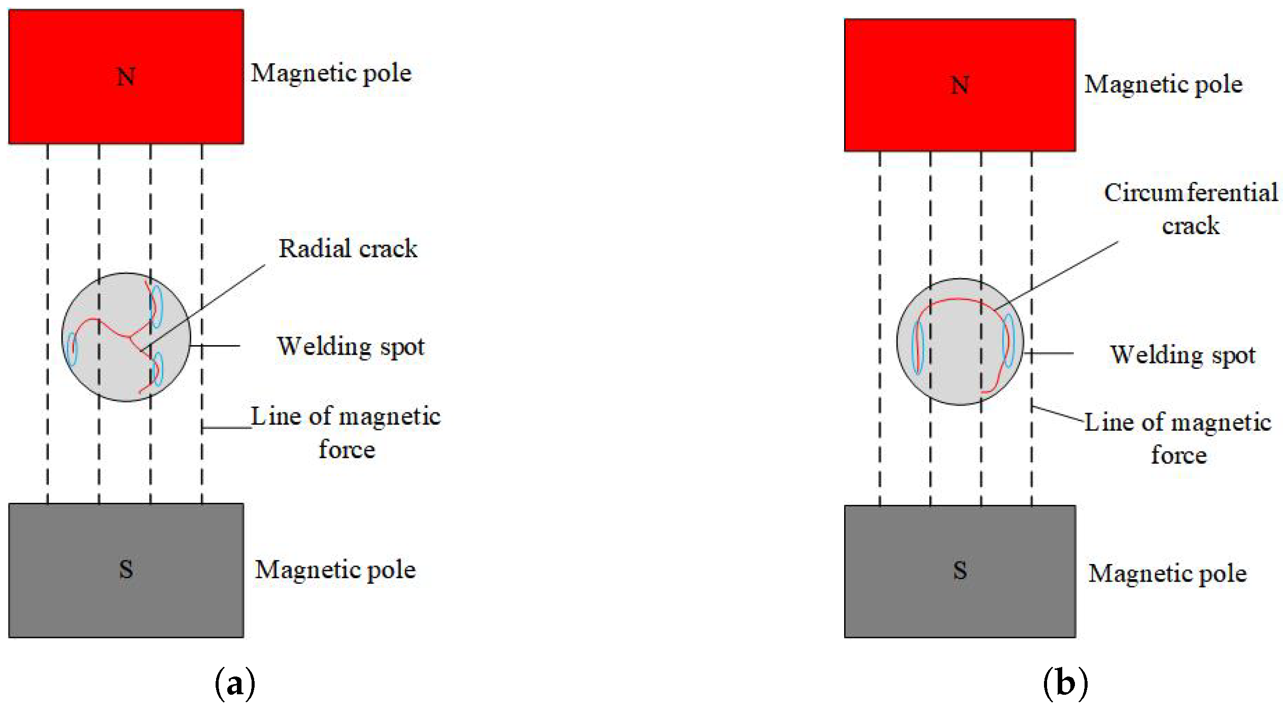
2. Simulation Analysis of Welding Defects

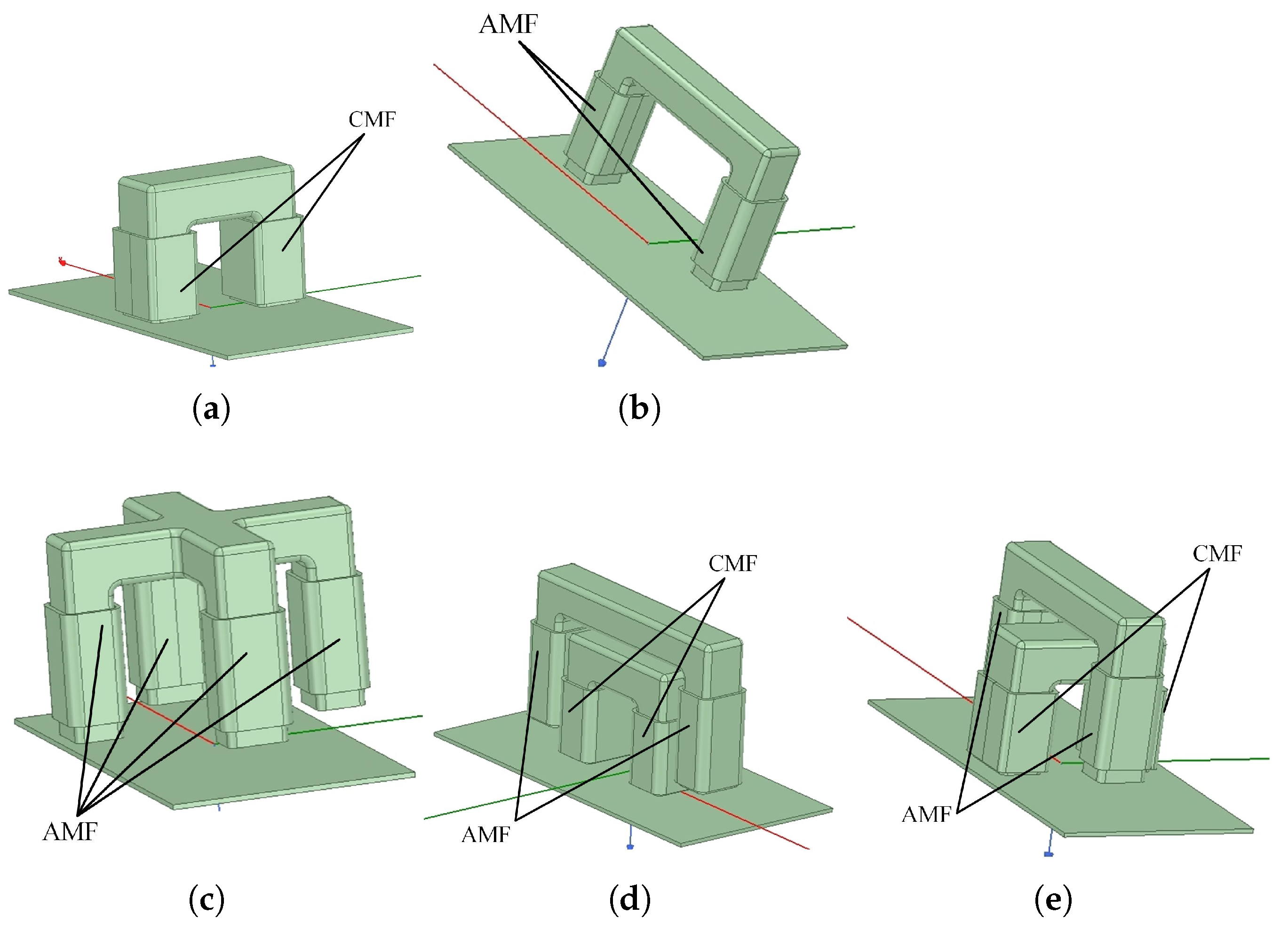
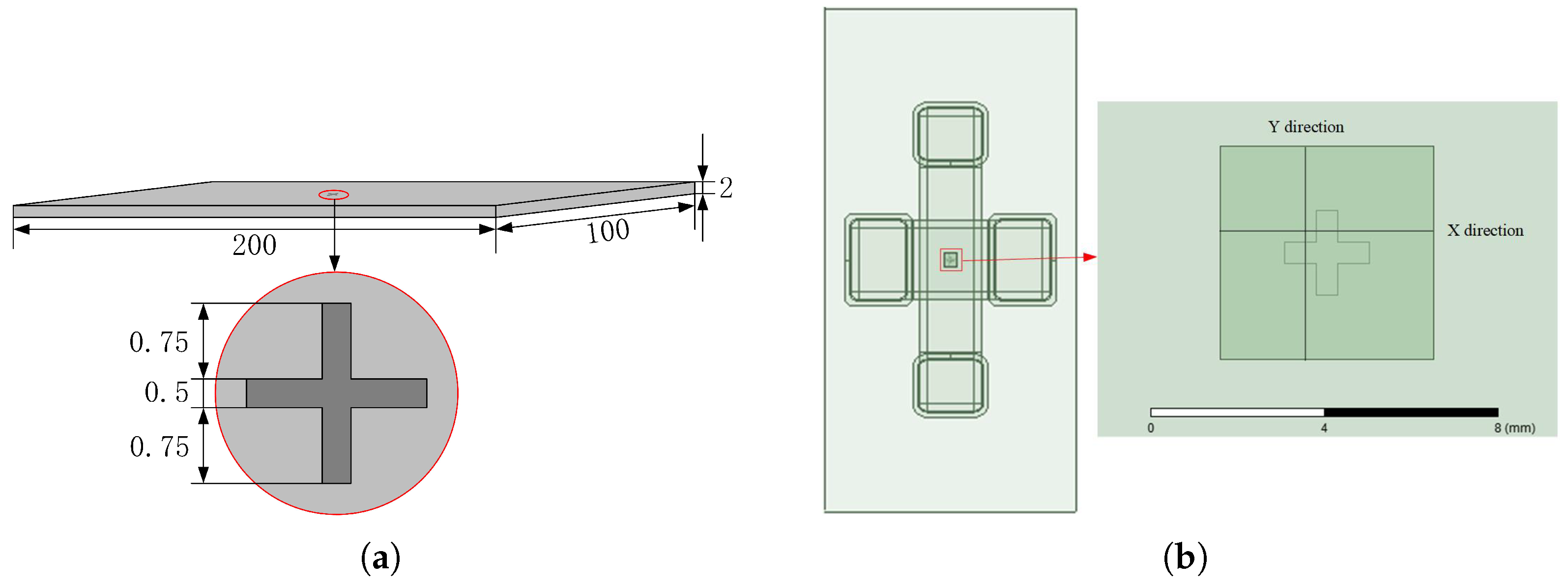
2.1. Establishment of Magnetic Field Simulation Models

Finite element simulation can be used as an auxiliary method to analyze the magnetic field distribution characteristics of spot welding defects [20,21]. In order to compare the magnetic leakage characteristics of defects under CMF, AMF, RMF, PCMF, and VCMF, and to verify the effect through magneto-optical imaging experiments, the defects of the tested samples in the simulation model are designed as cross-shaped surface grooves to simulate welding cracks. The simulation model and actual experimental device are first drawn in Pro/ENGINEER in a 1:1 ratio, and the model is then imported into Ansys Maxwell 18.0 for magnetic leakage characteristic analysis. The simulation models under different magnetic fields are shown in Figure 2.

In the electromagnetic simulation model in Figure 2, each excitation winding coil is set to 500 turns, which means that each pair of winding coils has 1000 turns. A steel plate model with cross grooves is used as the tested sample. The size of the tested sample and the size of the cross groove are shown in Figure 3a. The unit in the figure is mm, and the groove depth is 1 mm. When using the VCMF simulation model in Figure 2e, a small air domain was established above the cross recess. The size (length, width) of this air domain is shown in Figure 3b, and the dimensions in the figure are in millimeters. The thickness of the air domain is 0.2 mm. This processing method can save time for computer simulation models. Figure 3b is an enlarged view of the area where the local air domain is located. As shown in Figure 3b, there are two lines in the air domain, one in the X direction and the other in the Y direction, with a lifting degree of 0.25 mm.

The excitation current of each winding in the CMF is 100 A. The excitation current of each pair of windings in an AMF is set to the alternating current of $2000sin\left(100\pi \mathrm{t}\right)$ A. The excitation currents of two sets of windings in an RMF are set to the alternating currents of $2000sin\left(100\pi \mathrm{t}\right)$ A and $2000cos\left(100\pi \mathrm{t}\right)$ A, respectively, with a phase difference of 90 degrees between the excitation currents of the two sets of windings. The excitation current of each winding in a CMF combination is 100A, and the excitation current of the AC magnetic field winding pair is $2000sin\left(100\pi \mathrm{t}\right)$ A. The distribution maps of scalar equal magnetic density B-plane for each model are shown in Figure 4. The scalar equal magnetic density B-plane represents the absolute value of the ${\mathrm{M}}_z$(x, y, z) magnetization distribution.

In Figure 4a, it can be seen that the CMF poles are distributed horizontally; that is, the magnetic field direction is horizontally distributed. The magnetic induction intensity of the vertical groove of the cross groove is significantly greater than that of the horizontal groove, and the leakage magnetic field near the contour line of the horizontal groove is weak. As shown in Figure 4b, the AMF poles are distributed vertically; that is, the magnetic field direction is vertically distributed. The magnetic induction intensity of the transverse groove of the cross groove is significantly greater than that of the vertical groove, and the leakage magnetic field near the contour line of the vertical groove is weak. According to the results of Figure 4a,b, it can be seen that, under constant and AMF excitation, only when the distribution direction of small defects is perpendicular to the magnetic field direction is it easier to generate a leakage magnetic field and image it on the magneto-optical image. By comparing Figure 4b,c, it can be observed that the magnetic induction intensity of the transverse groove in Figure 4c is lower than that of the transverse groove in Figure 4b, while the magnetic induction intensity of the vertical groove is higher than that of the vertical groove in Figure 4b. Therefore, it can be seen in Figure 4b,c that the magnetic induction intensity of the detected sample under an AMF is stronger than that under an RMF when the magnitude of the excitation current is the same.

By comparing Figure 4b,d, it can be observed that the magnetic induction intensity of the transverse groove in Figure 4d is smaller than that of the transverse groove in Figure 4b, and the magnetic induction intensity of the vertical groove is also smaller than that of the vertical groove in Figure 4b. According to the theoretical analysis presented in [19], it can be concluded that the magnetic permeability of ferromagnetic materials increases to a certain extent under combined magnetic fields, resulting in an increase in magnetic flux. The increase in the magnetic flux of the detected sample in Figure 4d leads to a decrease in the leakage magnetic field. Therefore, there will be a phenomenon where the magnetic induction intensity of the horizontal and vertical grooves in Figure 4d is lower than that in Figure 4b. By comparing Figure 4b,e, it can be observed that the magnetic induction intensity of the transverse groove in Figure 4e is slightly smaller than that of the transverse groove in Figure 4b, while the distribution area is larger than that in Figure 4b. Moreover, the magnetic induction intensity of the vertical groove is also higher than that of the vertical groove in Figure 4b.

Observing Figure 4b,d,e, it can be seen that, compared to a single magnetic field (excited by a single constant or AMF), when the distribution direction of the constant and AMFs in the combined magnetic field is the same, the magnetic permeability of the tested sample increases and the defect leakage magnetic field decreases. When the distribution direction of the constant and AMFs in the combined magnetic field is perpendicular, the magnetic permeability of the tested sample increases, but the increase is smaller than the increase in magnetic permeability when the distribution direction of the constant and AMFs is the same. Compared to AMFs and PCMFs, VCMFs are more conducive to achieving defect imaging. By comparing Figure 4c,e, it can be observed that the magnetic induction intensity of the transverse groove in Figure 4e is higher than that of the transverse groove in Figure 4c, and the magnetic induction intensity of the vertical groove is also higher than that of the vertical groove in Figure 4b. According to the simulation results in Figure 4c,e, it can be seen that, under the same excitation source, the VCMF is easier to achieve magneto-optical imaging of small defects than the RMF.

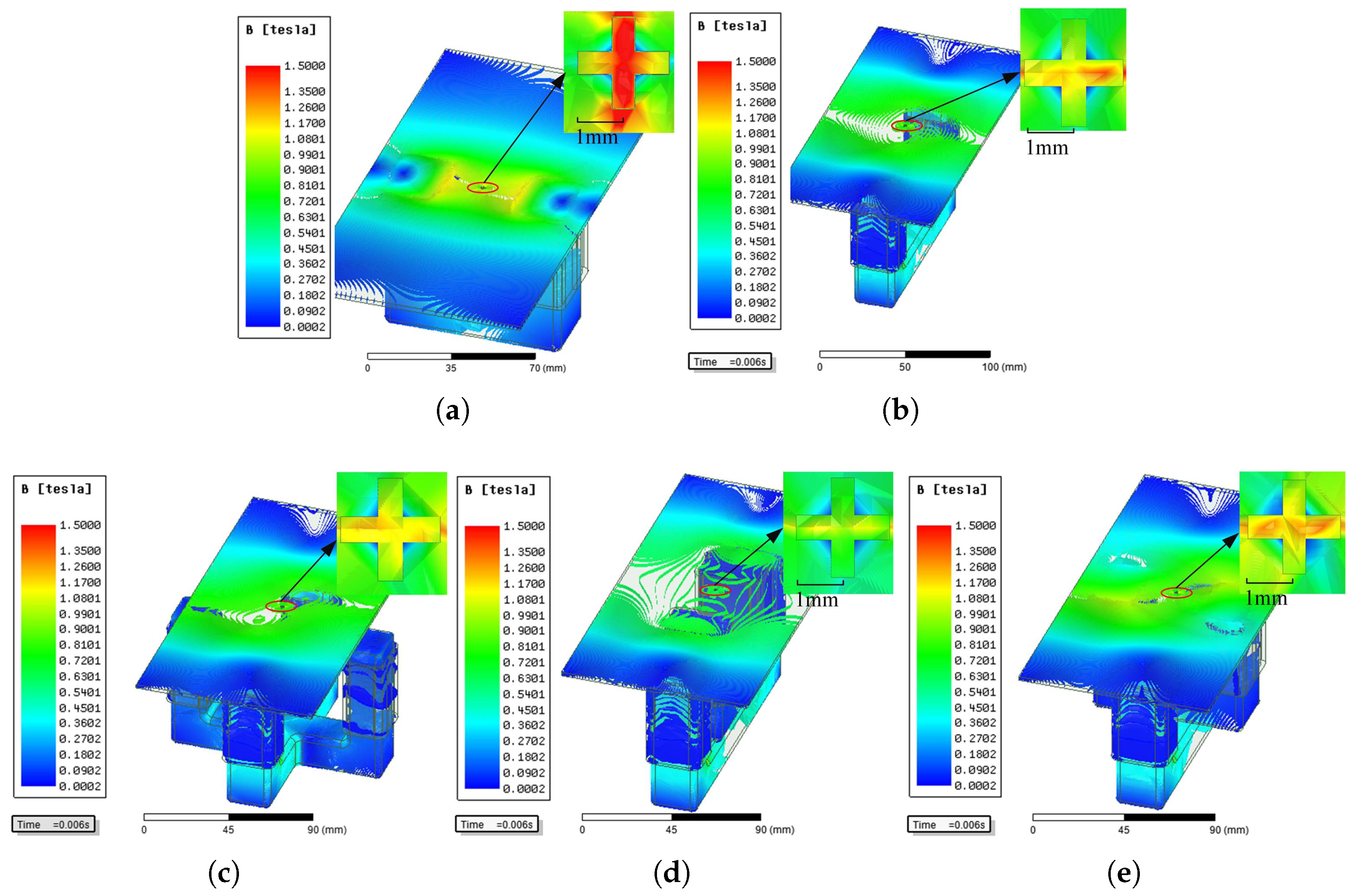
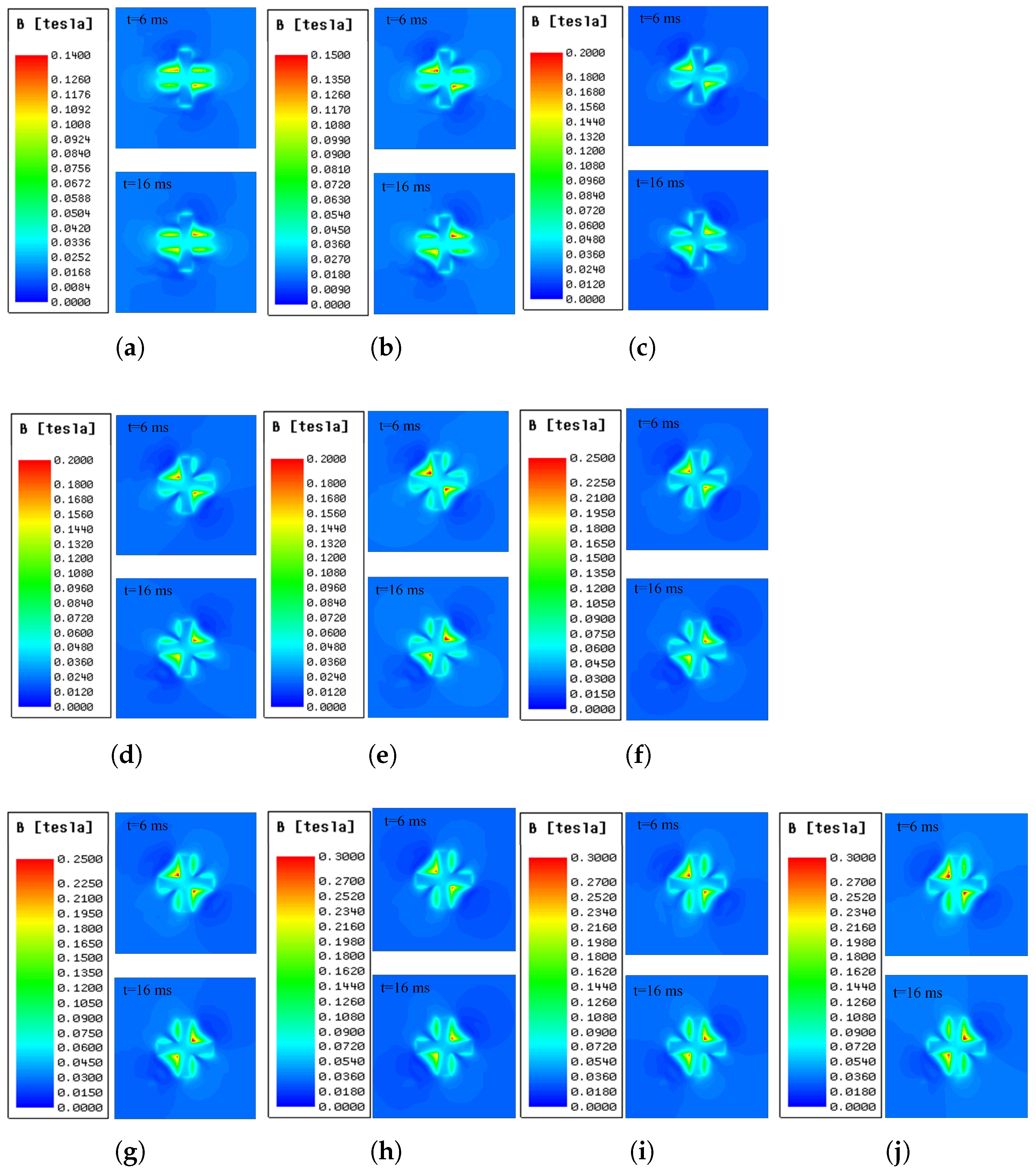
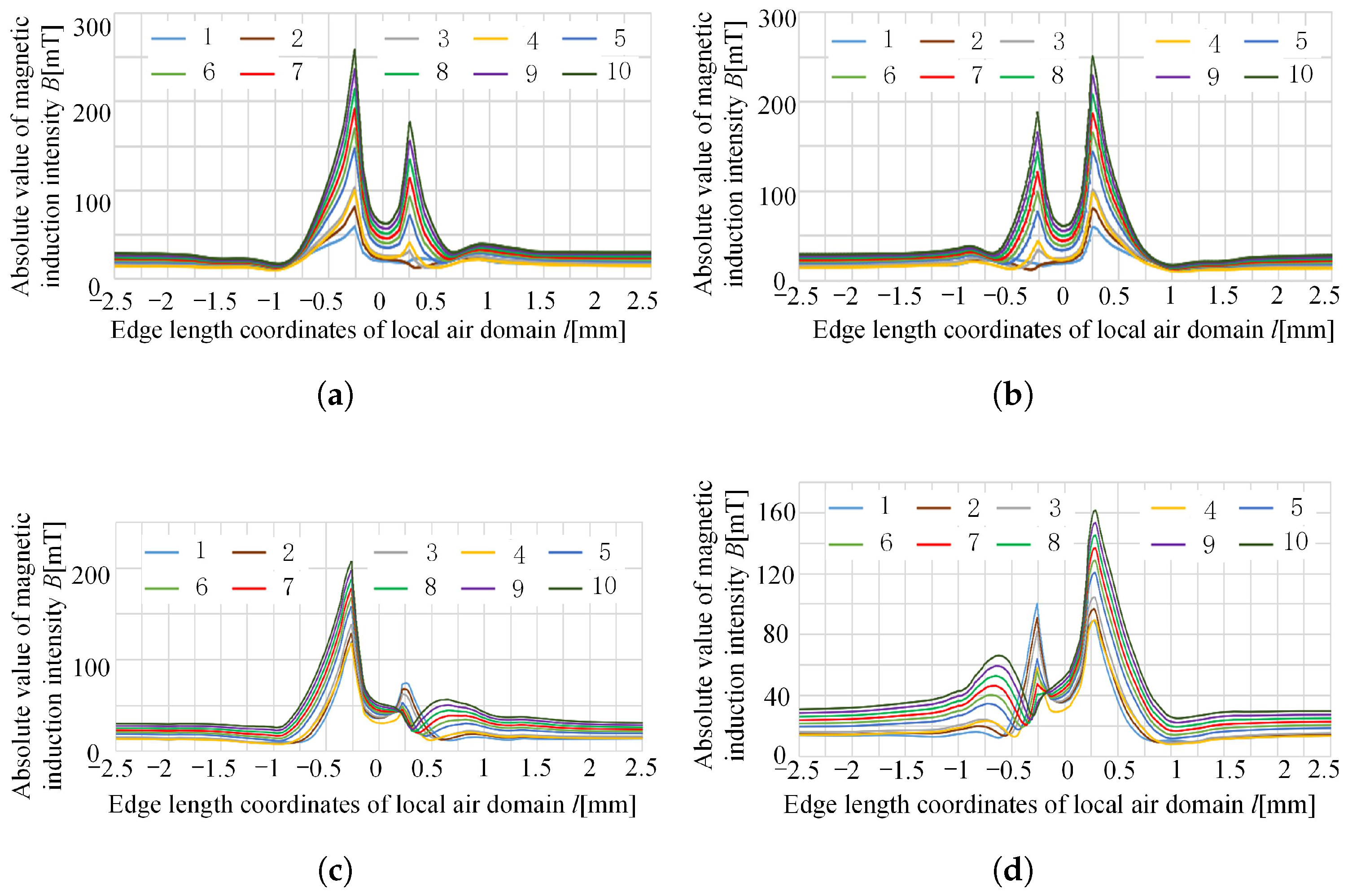
2.2. The Influence of CMF on the Characteristics of a Defect Leakage Magnetic Field

Based on the VCMF model in Section 2.1, the effect of changing the size of the CMF excitation source in the VCMF on the cross-recess leakage magnetic field under VCMF excitation was studied. The parameters of the constant and AMF excitation sources in the VCMF are shown in

Table 1. Type and size of the VCMF excitation source.

Serial Number of VCMF	AMF I[A]	CMF I[A]
1	100sin(100$\pi$t)	2
2		4
3		6
4		8
5		10
6		12
7		14
8		16
9		18
10		20

. The size of the AMF excitation source remains unchanged, and the CMF excitation source increases from 2 A to 20 A. Different sampling times were set, and the simulation sampling time points were 2, 4, 6, 8, 10, 12, 14, 16, 18, and 20 ms. At each sampling time point, the excitation current of the AMF in the VCMF is shown in Figure 5.

The B-plane diagram of equal magnetic density with a lift-off of 0.025 mm at sampling time points of 6 and 16 ms under different VCMFs is shown in Figure 6. The excitation source of the AMF in all VCMFs in the figure is $100sin\left(100\pi \mathrm{t}\right)$ A. In Table 1, it can be seen that the CMF excitation source in Figure 6a is 2 A. The CMF excitation source in Figure 6b is 4 A. The CMF excitation source in Figure 6c is 6 A, the CMF excitation source in Figure 6d is 8 A, the CMF excitation source in Figure 6e is 10 A, the CMF excitation source in Figure 6f is 12 A, and the CMF excitation source in Figure 6g is 14 A. The CMF excitation source in Figure 6h is 16 A. The CMF excitation source in Figure 6i is 18 A. The CMF excitation source in Figure 6j is 20 A.

The magnetic field intensity cloud map of the square area in Figure 3b is taken as the research object, and the lifting degree of the square area is set to 0.25 mm. Firstly, the magnetic density B-plane diagram of the cross groove under the VCMF in Figure 6 was divided into two groups for observation based on sampling times t = 6 ms and t = 16 ms. During the observation process, it was found that the contour of the transverse and longitudinal grooves in Figure 6a,b was blurry. The area where the transverse groove is located has strong magnetic induction, but it is difficult to define the boundary between the sample and the air domain. The magnetic induction intensity in the area where the longitudinal groove is located is weak, and there is a small difference in magnetic induction intensity between the samples on both sides of the defect contour and the air domain. The transverse and longitudinal grooves in Figure 6c–h have clear contours. However, the contour of the cross grooves in these figures has undergone a certain degree of deviation. The contour of the transverse and longitudinal grooves in Figure 6i,j is blurry. The area where the longitudinal groove is located has strong magnetic induction intensity, but it is difficult to define the boundary between the sample on both sides of the defect contour and the air domain. The magnetic induction intensity in the area where the transverse groove is located is weak, and there is a small difference in magnetic induction intensity between the samples on both sides of the defect contour and the air domain. According to the magnetic density B-plane diagram of the cross groove under the VCMF in Figure 6, it can be seen that the VCMF formed by the combination of a CMF in the horizontal direction and an AMF in the vertical direction can form an equal magnetic density B-plane distributed along the diagonal direction of the local air domain. That is to say, the distribution of magnetic field lines in a VCMF is approximately at a 45-degree angle to the original magnetic field. In Figure 6, it can be seen that the VCMF composed of a CMF excitation source of 12 A and an AMF excitation source of $100sin\left(100\pi \mathrm{t}\right)$A is more conducive to defect leakage detection.

The curve of the absolute value of magnetic induction intensity on the line with a lift-off of 0.025 mm under different vertical combinations of magnetic fields when changing the CMF is shown in Figure 7. When the sampling time is 6 ms, the absolute value of magnetic induction intensity on the X-direction line with a lift-off of 0.025 mm is shown in Figure 7a; When the sampling time is 16 ms, the absolute value of magnetic induction intensity on the X-direction line with a lift-off of 0.025 mm is shown in Figure 7b; When the sampling time is 6 ms, the absolute value of magnetic induction intensity on the Y-direction line with a lift-off of 0.025 mm is shown in Figure 7c; When the sampling time is 16 ms, the absolute value of magnetic induction intensity on the Y-direction line with a lift-off of 0.025 mm is shown in Figure 7d. The numbers 1–10 in the legend of Figure 7 represent the serial numbers of the VCMF in Table 1.

In Figure 7a,b, it can be seen that the curve of the absolute value of magnetic induction intensity on the X-direction line shows a more significant difference between the leakage magnetic field intensity at the defect contour and the air domain leakage magnetic field intensity as the CMF intensity in the VCMF increases. In Figure 7c,d, it can be seen that the curve of the absolute value of magnetic induction intensity on the Y-direction line shows some differences in the leakage magnetic field intensity at the defect contour and in the air domain as the CMF intensity in the VCMF increases. As the CMF intensity increases, a new maximum value will appear on the side of the defect contour near the sample area, which increases with the CMF intensity. This phenomenon can lead to misjudgment of the defect contour. As shown in Figure 7c,d, the extreme points of the defect contour on the left side of Curve 7 are approximately equal to the extreme points of the pseudo contour. Curves 8, 9, and 10 also exhibit a phenomenon where the extreme points of the pseudo contour on the left side are greater than the extreme points of the defect contour. Based on Figure 6 and Figure 7, it can be seen that increasing the CMF in the combined magnetic field will actually weaken the difference in magnetic leakage at the defect, which is not conducive to defect magneto-optical imaging.

3. Magneto-Optical Imaging Under VCMF

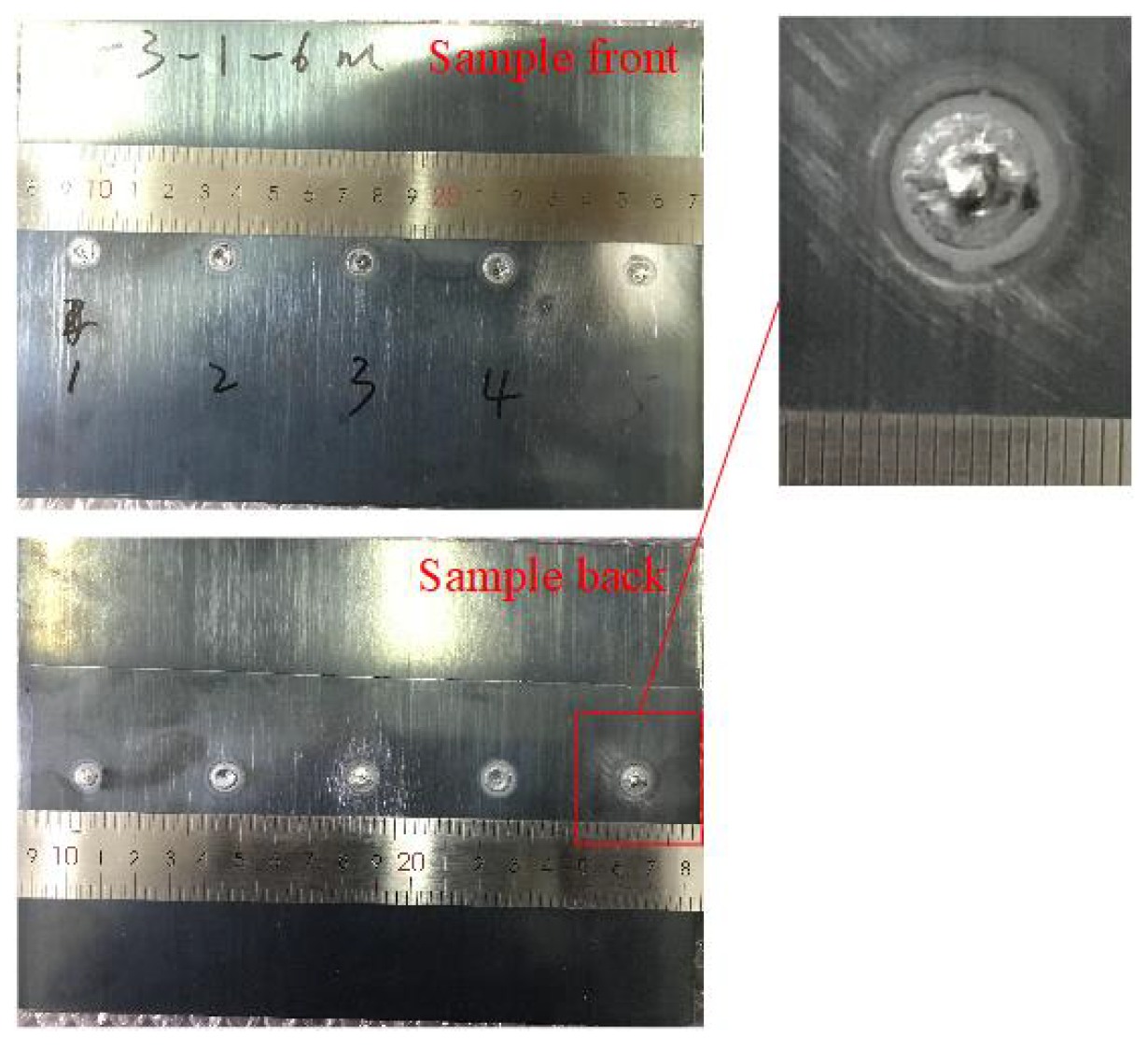
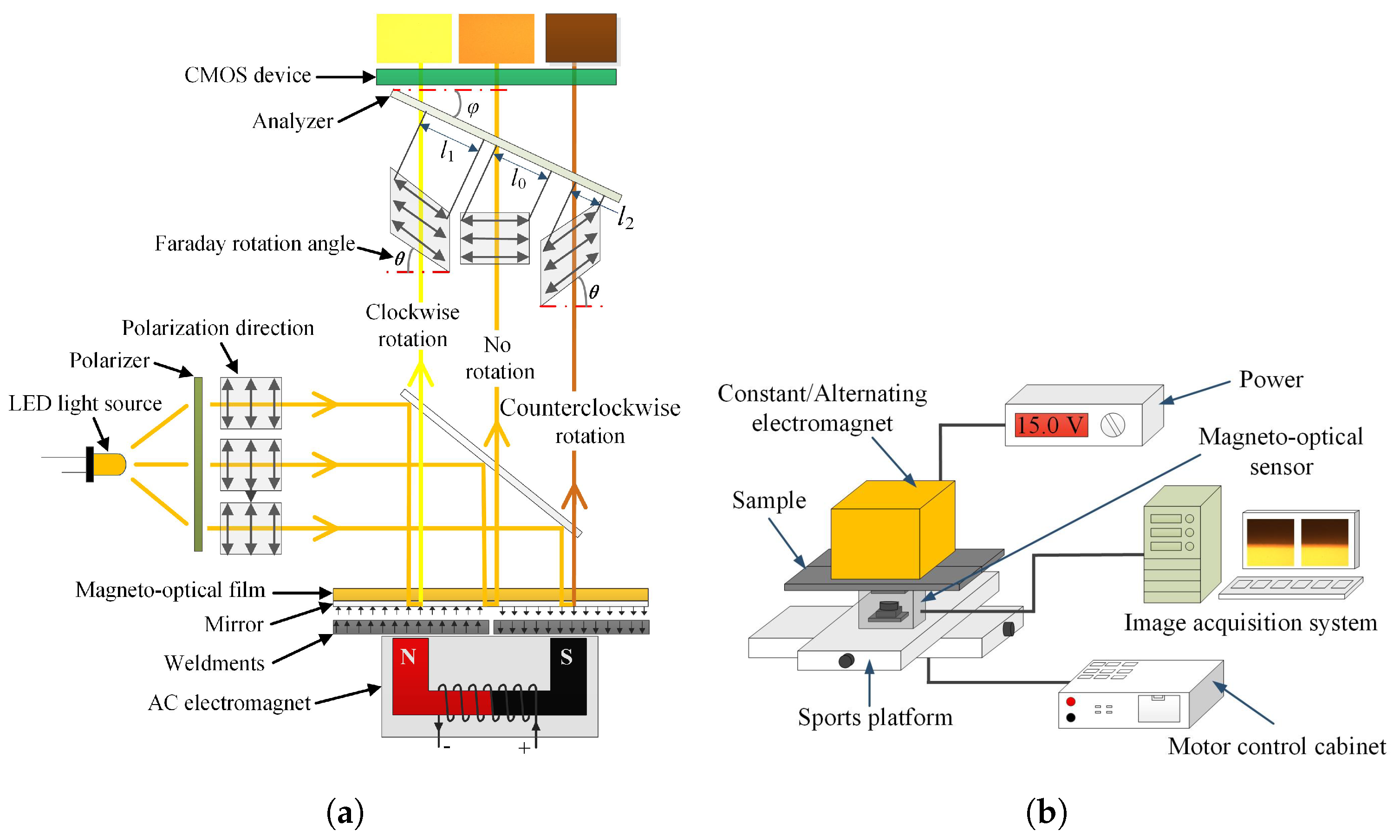
3.1. Magneto-Optical Imaging Testing Under VCMF

According to the simulation experiment in Section 2, it can be inferred that magneto-optical imaging non-destructive testing under VCMF excitation can achieve visual imaging of welding defects in any direction without strictly limiting the direction of the magnetic field. This section will study the effect of changes in a CMF in a VCMF on defect magneto-optical imaging through magneto-optical imaging experiments. After overlapping the medium carbon steel plate with a size of 200 × 100 × 1 mm, laser spot welding was used to obtain the test sample. The physical and locally enlarged images of the sample are shown in Figure 8. During the welding process, the protective gas flow rate is 20 L/min. The laser defocusing amount of solder joint is 10 mm, the welding time is 2.8 s, and the welding power is 1.6 kW. The principle of magneto-optical imaging and the experimental system of magneto-optical imaging are shown in Figure 9 [11].

As shown in Figure 9a, the magneto-optical imaging sensors are based on Faraday’s magneto rotation effect, which converts magnetic field intensity into a light intensity map to achieve visual imaging of magnetic fields. The light source emits a beam of monochromatic high-power light, which is polarized by a polarizer to become a beam of linearly polarized light. The magneto-optic film and reflective lens reflect the beam to obtain a beam of polarized light. The polarized light is detected by a polarizer and forms an intensity map in a complementary metal oxide semiconductor (COMS) imaging element. According to Faraday’s magneto rotation effect, linearly polarized light will rotate at different angles due to the magnitude of the magnetic field. The distance l traveled by light waves in a medium is proportional to the rotation angle $\theta$ of polarized light and the magnetic induction intensity component B in the direction of light propagation in the medium; that is,

$$\theta =VBl$$

(1)

and V is the Verdet constant.

Magneto-optical sensing is composed of magneto-optical thin films, complementary metal oxide semiconductors, light-emitting diodes, and optical conduction systems. The size of the magneto-optical film covered by the mirror coating in the magneto-optical sensor of this experimental system is 20$\times$15 ${\mathrm{mm}}^2$. Its main parameters include a light source wavelength of 590 nm, a sampling frequency of 8 to 100 frame/s, a maximum resolution of 2592$\times$1944 ${\mathrm{pixel}}^2$, a pixel calibration of 102 pixel/mm, and a magnetic field range of −2 to 2 kA/m. The magneto-optical imaging test system is shown in Figure 9b, which mainly includes an AC/DC power supply, an alternating magnetic field pole, a constant magnetic field pole, a platform control cabinet, a magneto-optical sensor, a magneto-optical imaging test platform, and a computer.

3.2. The Influence of the CMF on Magneto-Optical Imaging

To analyze the influence of changes in CMF intensity in a VCMF on the distribution of leakage magnetic field at the defect location of the tested sample, during the magneto-optical imaging experiment, the CMF size was changed while maintaining the same AMF size. The magneto-optical images of the tested samples obtained under CMF, AMF, and VCMF were compared and analyzed. The excitation voltage of the AMF was 15 V or 35 V, and the excitation voltage of the CMF was 1 V, 1.5 V, 2 V, and 2.5 V, respectively. The magneto-optical images obtained from a solder joint under the CMF, AMF, or VCMF are shown in

Table 2. Magneto-optical images of solder joint under different magnetic fields.

NMF	Excitation Voltage		Magneto-Optical Imaging
	CMF $\mathit{U}$ [V]	AMF $\mathit{U}$ [V]	F1	F2	F3
1	1	-
2	1.5	-
3	2	-
4	-	15
5	-	35
6	1	15
7	1.5	15
8	2	15
9	1.5	35

(In the table, NMF represents the number of magnetic fields). The sampling frequency for the magneto-optical imaging sensor was set to 75 frame/s. Therefore, the magneto-optical images obtained under AMF and VCMF excitation were 3 frames per cycle, as shown in Table 2.

In Table 2, it can be seen that, under the same excitation voltage, the magneto-optical images obtained from the solder joint under VCMF excitation are clearer than those obtained under single constant or AMF excitation, and the defects in the magneto-optical images are more obvious and complete. In the magneto-optical images obtained under VCMF excitation, as the CMF excitation source increases, the contour of defects in the magneto-optical images becomes increasingly obvious. From this, it can be seen that, under the same experimental conditions, the leakage magnetic field intensity of defects under a VCMF is stronger than that of a single CMF or AMF. The standard deviation of magneto-optical images in Table 2 is shown in

Table 3. Standard deviation of magneto-optical images of a solder joint under different magnetic fields.

NMF	Excitation Voltage		Magneto-Optical Imaging
	CMF  $\mathit{U}$ [V]	AMF  $\mathit{U}$ [V]	F1	F2	F3
1	1	-	9.71
2	1.5	-	12.39
3	2	-	24.98
4	-	15	17.62	19.69	13.10
5	-	35	27.18	19.38	19.78
6	1	15	17.77	13.24	12.14
7	1.5	15	15.51	28.34	20.50
8	2	15	17.95	30.47	23.15
9	1.5	35	18.70	40.18	32.10

.

Based on a CMF, an AMF perpendicular to its direction is added to form a VCMF. According to the values in Table 3, as the CMF increases, the minimum and intermediate values of the contrast of the magneto-optical images gradually increase, while the maximum values increase significantly. The contrast change of magneto-optical images obtained under a single CMF is from 9.71 to 12.39 to 24.98. Under the same AMF, as the CMF increases, the maximum contrast value of the magneto-optical image obtained by the VCMF changes from 17.77 to 28.34 to 30.47. These numerical results demonstrate that, under the excitation of a VCMF, the increase in a CMF is not linearly related to the increase in contrast of the magneto-optical image. After the CMF increases to a certain extent and its intensity continues to increase, there is no significant change in contrast to the magneto-optical image. The contrast change of magneto-optical images obtained under a single AMF is from 19.69 to 27.18. Under the same CMF intensity, as the AMF increases, the maximum contrast value of the magneto-optical image obtained by the VCMF changes from 28.34 to 40.18. These numerical results demonstrate that, under VCMF excitation, the increase in AMF is not linearly related to the increase in contrast of magneto-optical images, and the contrast of magneto-optical images changes more significantly than under a single AMF.

4. Conclusions

Through simulation experiments, it was found that not only would the contour of multi-angle weld defects under CMF or AMFs be missed, but they also would under PCMFs. The leakage magnetic field of defects under the RMF is not as strong as the leakage magnetic field of defects under a combined magnetic field, which can lead to poor magneto-optical imaging performance. Then, through simulation experiments, it was found that, as the CMF intensity increases, a new maximum value will appear on the side near the sample area of the defect contour. This maximum value increases with the increase of the CMF intensity, which can lead to misjudgment of the defect contour. Continuously increasing the CMF in the combined magnetic field will actually weaken the magnetic leakage difference at the defect site, which is not conducive to defect magneto-optical imaging. When the maximum value of the excitation current of the AMF is at least 12 times the excitation current of the CMF, there will be no false contour defects. Finally, magnetic-optical imaging experiments were conducted to verify that the information obtained from multi-angle welding defect detection under VCMFs is more comprehensive than that obtained under CMFs, AMFs, and PCMFs, and the defect magnetic-optical images obtained under VCMFs are clearer. The results indicate that using VCMF excitation can effectively improve the contrast of magneto-optical images. This can overcome the existing problem of difficult imaging of small defects in magneto-optical images under AMF excitation. This also helps to extract feature parameters during the defect recognition process.

References

1. Sun, J.; Li, C.; Wu, X.J.; Palade, V.; Fang, W. An Effective Method of Weld Defect Detection and Classification Based on Machine Vision. IEEE Trans. Ind. Inform. 2019, 15, 6322–6333. [Google Scholar] [CrossRef]
2. Liu, T.; Zheng, P.; Bao, J.; Chen, H. A state-of-the-art survey of welding radiographic image analysis: Challenges, technologies and applications. Measurement 2023, 214, 112821. [Google Scholar] [CrossRef]
3. Liu, W.; Shan, S.; Chen, H.; Wang, R.; Sun, J.; Zhou, Z. X-ray weld defect detection based on AF-RCNN. Weld. World 2022, 66, 1165–1177. [Google Scholar] [CrossRef]
4. Górka, J.; Jamrozik, W. Enhancement of Imperfection Detection Capabilities in TIG Welding of the Infrared Monitoring System. Metals 2021, 11, 1624. [Google Scholar] [CrossRef]
5. Sun, H.; Ramuhalli, P.; Jacob, R.E. Machine learning for ultrasonic nondestructive examination of welding defects: A systematic review. Ultrasonics 2023, 127, 106854. [Google Scholar] [CrossRef] [PubMed]
6. Honarvar, F.; Varvani-Farahani, A. A review of ultrasonic testing applications in additive manufacturing: Defect evaluation, material characterization, and process control. Ultrasonics 2020, 108, 106227. [Google Scholar] [CrossRef] [PubMed]
7. Kumar, S.; Wu, C.; Padhy, G.; Ding, W. Application of ultrasonic vibrations in welding and metal processing: A status review. J. Manuf. Process. 2017, 26, 295–322. [Google Scholar] [CrossRef]
8. Gholizadeh, S. A review of non-destructive testing methods of composite materials. Procedia Struct. Integr. 2016, 1, 50–57. [Google Scholar] [CrossRef]
9. Fitzpatrick, G.L.; Thome, D.K.; Skaugset, R.L.; Shih, E.Y.; Shih, W.C. Magneto-optic/eddy current imaging of aging aircraft: A new NDI technique. Mater. Eval. 1993, 51, 1402–1407. Available online: https://www.osti.gov/biblio/5044997 (accessed on 9 February 2025).
10. Gao, X.; Mo, L.; You, D.; Li, Z. Tight butt joint weld detection based on optical flow and particle filtering of magneto-optical imaging. Mech. Syst. Signal Process. 2017, 96, 16–30. [Google Scholar]
11. Gao, X.; Lan, C.; You, D.; Li, G.; Zhang, N. Weldment nondestructive testing using magneto-optical imaging induced by alternating magnetic field. J. Nondestruct. Eval. 2017, 36, 55. [Google Scholar] [CrossRef]
12. Li, D.; Han, Z.; Zhao, P.; Dong, Z.; Zhao, S.; Zhu, R.; Li, F.; Yang, Y.; Lin, X. Laser welding by focusing multi-laser beams. Opt. Express 2024, 32, 23147–23160. [Google Scholar] [CrossRef] [PubMed]
13. Alghannam, E.; Lu, H.; Ma, M.; Cheng, Q.; Gonzalez, A.A.; Zang, Y.; Li, S. A Novel Method of Using Vision System and Fuzzy Logic for Quality Estimation of Resistance Spot Welding. Symmetry 2019, 11, 990. [Google Scholar] [CrossRef]
14. Xu, H.; Yan, Z.; Ji, B.; Huang, P.; Cheng, J.; Wu, X. Defect detection in welding radiographic images based on semantic segmentation methods. Measurement 2022, 188, 110569. [Google Scholar] [CrossRef]
15. Naddaf-Sh, M.M.; Naddaf-Sh, S.; Zargarzadeh, H.; Zahiri, S.M.; Dalton, M.; Elpers, G.; Kashani, A.R. Defect detection and classification in welding using deep learning and digital radiography. In Fault Diagnosis and Prognosis Techniques for Complex Engineering Systems; Elsevier: Amsterdam, The Netherlands, 2021; pp. 327–352. [Google Scholar] [CrossRef]
16. Sazonova, S.A.; Nikolenko, S.D.; Osipov, A.A.; Zyazina, T.V.; Venevitin, A.A. Weld defects and automation of methods for their detection. J. Phys. Conf. Ser. 2021, 1889, 022078. [Google Scholar] [CrossRef]
17. Tsukada, K.; Miyake, K.; Harada, D.; Sakai, K.; Kiwa, T. Magnetic nondestructive test for resistance spot welds using magnetic flux penetration and eddy current methods. J. Nondestruct. Eval. 2013, 32, 286–293. [Google Scholar] [CrossRef]
18. Zhao, D.; Ivanov, M.; Wang, Y.; Du, W. Welding quality evaluation of resistance spot welding based on a hybrid approach. J. Intell. Manuf. 2021, 32, 1819–1832. [Google Scholar] [CrossRef]
19. Ma, N.; Gao, X.; Wang, C.; Zhang, Y. Optimization of Magneto-Optical Imaging Visualization of Micro-Defects Under Combined Magnetic Field Based on Dynamic Permeability. IEEE Trans. Instrum. Meas. 2021, 70, 1–9. [Google Scholar]
20. Xu, Z.; Zha, X.; Chen, H.; Sun, Y.; Long, M. A simulation study for locating defects in tubes using the weak MFL signal based on the multi-channel correlation technique. Insight-Non-Destr. Test. Cond. Monit. 2015, 57, 518–527. [Google Scholar] [CrossRef]
21. Zheng, X.; Zhu, S.; Zhang, X.; Shen, B. Compressing magnetic field into a high-intensity electromagnetic field with a relativistic flying mirror. Opt. Express 2021, 29, 41121–41131. [Google Scholar] [CrossRef]
Figure 1. Distribution of spot welding cracks and magnetic field. (a) Radial cracks in spot welding, (b) Circumferential cracks in spot welding.
Metals 15 00340 g001
Figure 2. Simulation model of an electromagnet. (a) CMF, (b) AMF, (c) RMF, (d) PCMF, and (e) VCMF.
Metals 15 00340 g002
Figure 3. Simulation model. (a) Tested sample in the simulation model (unit: mm). (b) Top view of local air domain.
Metals 15 00340 g003
Figure 4. B-plane and local magnified images of simulation models with equal magnetic density under different magnetic fields. (a) CMF, (b) AMF, (c) RMF, (d) PCMF, and (e) VCMF.
Metals 15 00340 g004
Figure 5. Excitation current of two pole pairs at each sampling time point.
Metals 15 00340 g005
Figure 6. Plane B of equal magnetic density under different VCMFs when changing the CMF. (a) VCMF 1, (b) VCMF 2, (c) VCMF 3, (d) VCMF 4, (e) VCMF 5, (f) VCMF 6, (g) VCMF 7, (h) VCMF 8, (i) VCMF 9, and (j) VCMF 10.
Metals 15 00340 g006
Figure 7. Absolute value of magnetic induction intensity on the lower line of different VCMFs when changing the CMF. (a) The X-direction line at a sampling time of 6 ms, (b) the X-direction line at a sampling time of 16 ms, (c) the Y-direction line at a sampling time of 6 ms, and (d) the Y-direction line at a sampling time of 16 ms.
Metals 15 00340 g007
Figure 8. Physical drawing and partial enlarged drawing of laser spot welding sample.
Metals 15 00340 g008
Figure 9. Magneto-optical imaging detection. (a) Detection principle. (b) Schematic diagram of the experimental platform.
Metals 15 00340 g009