Structural Integrity and Life Assessment of Ti-6Al-4V Orthopaedic Implants

Abstract

This paper presents an experimental and numerical analysis of the mechanical behaviour of orthopaedic implants with crack-type defects, considering the principles and advantages of the modern X-FEM method, which was used due to limitations of traditional FEM in terms of crack growth simulation, especially for complex geometries. In X-FEM, the finite element space is enriched with discontinuity functions and asymptotic functions at the crack tip, which are integrated into the standard finite element approximation using the unity division property. Though rare, femoral component failures are well-documented complications that can occur after hip prosthetic implantation. Most stem fractures happen in the first third of the implant due to the loosening of the proximal stem and fixation of the distal stem, leading to bending and eventual fatigue failure. The main goal of this paper was to obtain accurate and representative models of such failures. Experimental analyses of the mechanical behaviour of implants subjected to physiological loads, according to relevant standards, using a new combined approach, including both experiments and numerical simulations was presented. The goal was to verify the numerical results and obtain a novel, effective methodology for assessing the remaining fatigue life of hip implants. For this purpose, the analysis of the influence of Paris coefficients on the total number of cycles was also considered. Hence, this simulation involved defining loads to closely mimic real-life scenarios, including a combination of activities such as ascending stairs, stumbling, and descending stairs. The tensile properties of the titanium alloy were experimentally determined, along with the Paris law coefficients C and m. The finite element software ANSYS 2022R2 version was used to develop and calculate the three-dimensional model with a crack, and the resulting stresses, stress intensity factors, and the number of cycles presented in the figures, tables, and diagrams. The results for the fatigue life of a partial hip implant subjected to various load cases indicated significant differences in behaviour, and this underscores the importance of analysing each case individually, as these loads are heavily influenced by each patient’s specific activities. It was concluded that the use of numerical methods enabled the preliminary analyses of the mechanical behaviour of implants under fatigue loading for several different load cases, and these findings can be effectively used to predict the possibility of Ti-6Al-4V implant failure under variable cyclic loads.

1. Introduction

By using metallic alloys, along with high-grade plastics and polymers, orthopaedic surgeons can reconstruct fractured hips, or replace a painful, dysfunctional joint with a highly functional long-lasting prosthetic. However, the largest number of implants have a lifespan of 10–15 years. One of the most common issues, both for doctors and patients, is the tendency of these implants to fail [1,2,3,4]. There are many influencing factors that could lead to the failure of orthopaedic implants [5,6,7,8,9], although fracture due to fatigue and wear was identified as one of the main problems related to the loosening of the bone–prosthetic connection and implant fracture. Figure 1 shows examples of a hip implant prosthetic fracture caused by fatigue [10]. It can be seen that the interaction of fatigue and wear played a significant part in the failure of this biomedical equipment.

The failure of femoral components is a rare but also a well-documented complication which can occur after the hip prosthetic is implanted. Most stem fractures occur at the first third of the implant, where the loosening of the proximal stem and the fixation of the solid distal stem result in bending, which ultimately leads to fatigue failure [11,12].

The failure analyses of femoral components identified several contributing factors, including implant material, type and positioning, cementing technique, and loading [13,14,15].

In general, the human body is the most sensitive to fatigue in joints, wherein applied biomaterials can withstand a large number of work cycles, with an order of magnitude between 10 and 100 million. This is a very difficult condition for any synthetic biomaterial to fulfil. The long-term response of the body to implant materials is another notable issue, especially when the residue created by wear is not biodegradable.

In order to solve these issues, surgeons and bioengineers defined a number of design requirements, along with favourable properties of adequate biomaterials. The demands that prosthetic joints need to meet are highly complex due to specific functional requirements and critical limitations of currently available biomaterials and models. Apart from the limited selection of adequate materials, prosthetic joints must also function in an adverse environment, while being subjected to high-level loads.

Efficiency of biomaterials within the body depends on various factors such as its properties and biocompatibility, along with other aspects, which are not under the engineer’s control, including surgical techniques, health condition, and activity of the patient.

Hence, although one mode of failure could be controlled (e.g., resistance to fracture), other means of failure, such as infections, can significantly limit the usefulness of data about total implant reliability. The basic condition that every biomedical construction must satisfy is safety and reliability in the conditions of exploitation. In order to meet this condition, the properties of the geometry and material from which the implant is made are crucial. Titanium alloys are known for their high sensitivity to fatigue due to the presence of cracks or notches. Consequently, the components of the prosthesis must be analysed for the possibility of damage and cracks in places of maximum stress concentration.

As part of the research on this type of partial hip prosthesis, experimental analyses based on 3D optical measurements were performed, using the digital image correlation (DIC) methodology [16,17,18]. In order to analyse the mechanical behaviour of the prosthesis and determine the strain and displacement fields, experimental tests were performed based on the ISO 7206-4 standard [19]. The main goal of the experimental research was to determine the correlations between load and displacement, with the highest displacement and strain values obtained in areas where failures occurred in real implants, which also coincides with the numerically obtained values of the stress field and critical locations where maximum stresses can occur [18].

ISO 7206-4 standard was applied, which defines laboratory tests for determining the durability properties of the femoral component of the hip prosthesis. The defined testing method is based on several assumptions in order to reduce the complexity of the problem to a repeatable test. One of the objectives of the conducted research was to examine the influence of the difference in the load defined in the ISO 7206-4 standard and the simulated physiological loads that occur in vivo on the mechanical behaviour of the implant, which can lead to crack propagation and eventual failure.

Another important contribution of this research is the use of the numerical simulation of the fatigue behaviour of titanium alloy hip implants, which is based on experimentally obtained results. These simulations allowed for the further optimization of the models, by determining which of the experimentally obtained input parameters (Paris law coefficients) are the most critical, in terms of resistance to fatigue crack growth.

Finite element analysis is often used for the purpose of assessing the effect of initial defects in the material on its strength and work life, since it can consider various crack geometries, dimensions, and locations. However, classic FEM is somewhat limited in this area, since changes in crack topology require the generating of new meshes for each step of its propagation. This can lead to complications when analysing crack propagation in complex geometries. For this reason, a new version of FEM was developed and named the Extended Finite Element Method (XFEM), of which the main goal was to eliminate the need for repeated mesh generation. This research relied on the state-of-the-art applications of FEM in order to efficiently obtain results which have shown very good agreement with the results obtained by previous research, including experiments and DIC.

This numerical approach, that simulates the entire process of crack propagation which is not so present in the literature, represents an innovative approach to predict implant behaviour, and can be used as a preliminary analysis where defects in the material and the crack initiation could be expected. Hence, this approach represents a combination of experimental and numerical methods, which provided verified numerical models in accordance with standard implant testing recommendations. It also considers the influence of experimentally determined parameters of fracture mechanics, i.e., the Paris equation, on the results of numerical analyses, allowing for the determination of which combination of parameters is the most critical.

2. Extended Finite Element Method for Fatigue Fracture Analysis

The basis of this method was defined by Belytschko and Black [20], as well as Moës et al. [21]. The Extended Finite Element Method uses enrichment functions which simulate discontinuities in structures (namely cracks), along with asymptotic functions near the crack tip, which introduce additional degrees of freedom via the Partition of Unity [22].

Essentially, XFEM is based on well-known FEM procedures, combined with improvements which, in turn, are based on the Partition of Unity finite element method (PUFEM) [22]. In addition, it introduces enrichment functions in order to better represent displacement in the crack domain. Due to this, XFEM approximations and enrichments are only applied at a local level, for a small number of finite elements, instead of being used globally for the whole model. This is another advantage of the method, since using it on the model as a whole would make the analysis a lot more complex and time consuming. All of the analyses which are presented in the paper were performed for the purpose of determining the fatigue behaviour of orthopaedic implants, and the obtained results could prove useful in the predicting of potential failure and prevention of catastrophic implant fracture.

Extended finite element method is widely used in numerical simulations which involve fatigue crack growth, which is not surprising, considering this was one of the main reasons for developing the method in the first place. A number of examples of numerical simulations using XFEM can be found in the literature [23,24,25,26,27,28]. This method resolved the issues which were encountered when attempting to use the classic FEM approach for the modelling of cracks, by using enrichment functions in order to introduce discontinuities to the FE models. The method itself is based on the concept of Partition of Unity [22], which in turn relies on the introduction of the so called enrichment functions. The purpose of these functions is to “override” the issue of discontinuities such as cracks by approximation of finite elements in the vicinity of the crack. These approximations, related to displacements around the crack, have the following form:

$${\mathrm{u}}_{\mathrm{xfem}}\left(\mathrm{x}\right)={\displaystyle \sum _{i\in I}{N}_i\left(\mathrm{x}\right){\mathrm{u}}_i}+{\displaystyle \sum _{i\in J}{N}_i\left(\mathrm{x}\right)H\left(\mathrm{x}\right){\mathrm{a}}_i}+{\displaystyle \sum _{i\in K}\left[N_i\left(\mathrm{x}\right){\displaystyle \sum _{\alpha =1}^4{F}_{\alpha }\left(\mathrm{x}\right){\mathrm{b}}_{i\alpha }}\right]}$$

(1)

where I is the set of all nodes in the finite element mesh, N_i(x) is the shape function for each node, and u_i is the degrees of freedom. H(x) is the Heavyside function, one of the most commonly used forms of enrichment functions, and is defined as

$$H\left(\xi ,\eta ,\zeta \right)=\left\{\begin{array}{c}+1:\phi \left(\xi ,\eta ,\zeta \right)>0\\ -1:\phi \left(\xi ,\eta ,\zeta \right)<0\\ \pm 1:\phi \left(\xi ,\eta ,\zeta \right)=0\end{array}\right.$$

(2)

where H is the Heavyside function, and ξ, η and ζ are the coordinates. This function is combined with the level-set fields, which are used to define the crack surface (and in the case of a three-dimensional problem, the crack front). Level-set fields are defined as follows:

$$\varphi \left(\xi ,\eta ,\zeta \right)={\displaystyle {\sum }_i{N}_i\left(\xi ,\eta ,\zeta \right){\Phi }_i}$$

(3)

where Φ_i is the nodal values of the level set function.

In addition to the above, another type of enriched nodes is used at the crack tip, since it is more accurate at approximating discontinuities compared to the Heavyside function, i.e., the Near Tip (NT) nodes, which have additional degrees of freedom (for a total of 10 DOFs).

Regarding fatigue crack growth, XFEM mainly relies on the well-known Paris Equation [29], which is given below in its simplest form (Equation (4)):

$${\displaystyle \frac{da}{dN}}=C\cdot \Delta K^m$$

(4)

This equation also has various modified forms, such as the one shown in [30], but for the purpose of the analysis shown in this paper, the above version of the Paris law was sufficient. The most important factors in XFEM analyses are the coefficient C and exponent m, which should be determined experimentally as they can significantly differ even in cases of test specimens which were all taken from the same batch of material [31]. Values of C and m are then used as input data for the simulation, along with the mechanical properties of the material. Regarding the ΔK, the stress intensity factor range, in this case, it is based on K_I, i.e., the SIF value for the first crack opening mode, which corresponds to real fatigue crack propagation in hip implants. Stress intensity factor is calculated according to the following formula:

$$K_I=Y\cdot \sigma \cdot \sqrt{\pi \cdot a}$$

(5)

where Y is the geometry factor, which depends on the shape and location of the crack (this coefficient would be typically determined according to the recommendation given in [32]; however, ANSYS uses the interaction integral method [33] to perform the stress–intensity factor calculation, also based on crack position, length, and geometry), σ is the stress and a represents crack length [34]. Using XFEM with the previously explained input parameters enables a relatively simple and effective means of calculating the stress intensity factors along the fatigue crack front, which was one of the goals of the simulations presented here. Additionally, XFEM analyses can provide valuable insight into the number of cycles and critical crack lengths, thus for allowing detailed fatigue crack growth predictions.

The calculations in this case were performed in ANSYS software, and this method requires the defining of a certain number of load steps. Load steps determine how much the fatigue crack can grow, which means that their total number defines the maximum crack growth in the model. For this reason, it is important to define the correct number of steps until critical crack length is reached, and this will be explained in more details in the chapter where the numerical model development is described.

A notable advantage of using this method for fatigue simulation is the ease with which numerous parameters of the model can be varied, including loads, crack geometry and length/depth, finite element mesh size, and, of course, input data such as Paris coefficients, yield stress, tensile strength, etc. This way, multiple load cases, both in terms of type (walking, climbing stairs, stumbling) and patient weight, can be included in the calculations, without requiring any significant efforts in creating new models.

The application of XFEM to the fatigue calculation of such structures does have its disadvantages, mainly reflected in the fact that it relies heavily of experimental tests in order to obtain proper Paris coefficients, i.e., the C and m values.

3. Experimental Testing

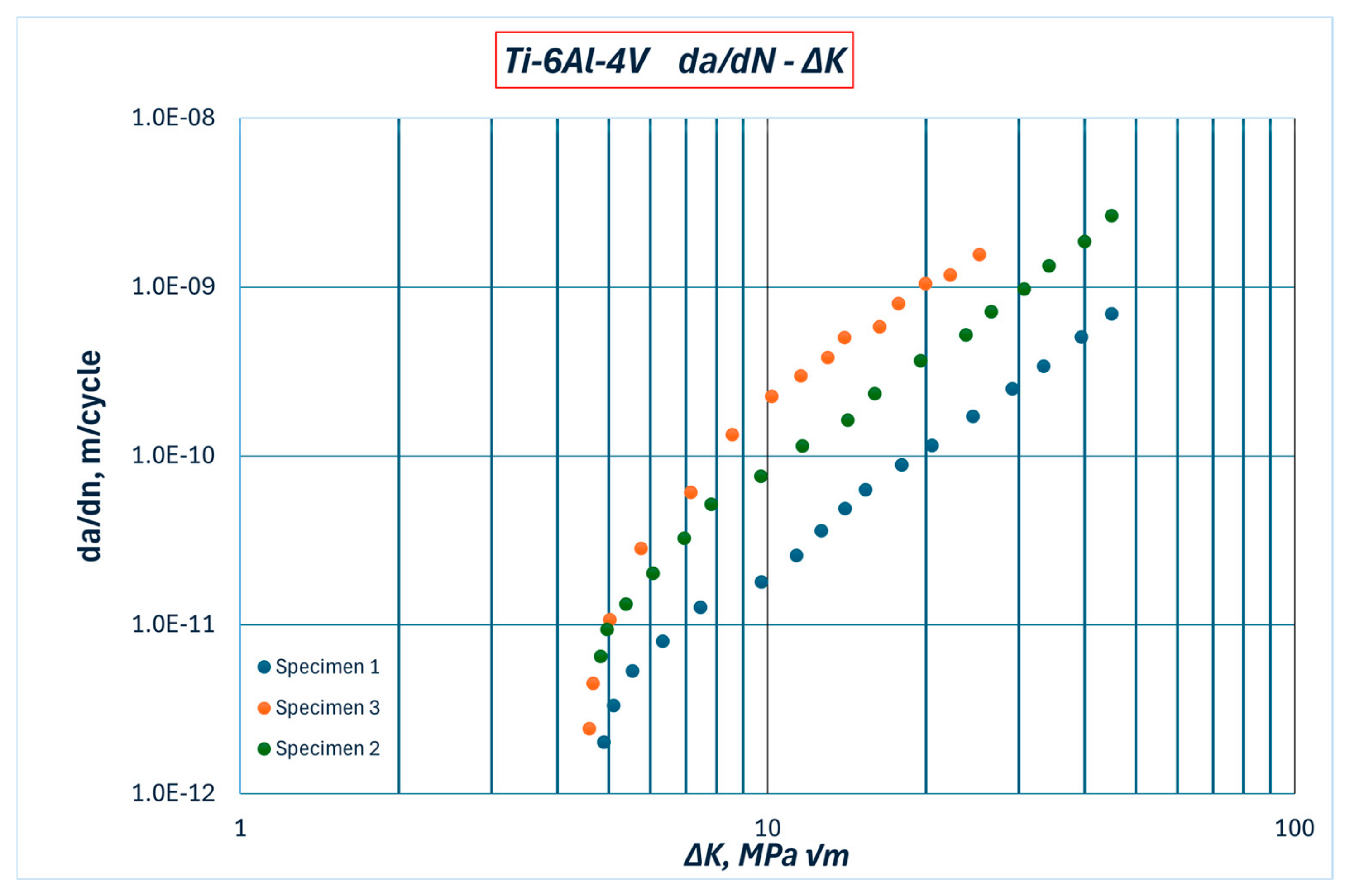
The Paris coefficients for these models were previously determined experimentally, as reported in [31], based on da/dN—ΔK curves, as shown in Figure 2. That study [31] involved three different specimens, and the relevant combination that was adopted was the least favourable one (Specimen 2), as a part of a conservative approach.

The experimental analysis of titanium alloy implants presented in this paper is based on the modification of the standard for testing biomedical prostheses. In order to analyse the mechanical behaviour of the prosthesis under physiological load, the experimental conditions were based on the ISO 7206-4 standard, which is used to determine the resistance of the femoral components of hip prostheses. Loads were selected based on the relevant standards, as well as data available from the literature. Therefore, the aim of this study was to analyse the impact of higher load values on the stability and integrity of the implant, which can occur in vivo, and which can affect the propagation of the crack in the material and the final failure of the implant.

Measuring systems for optical three-dimensional deformation analysis represent the most modern measuring method for understanding the mechanical behaviour of biomaterials and components independent of the material, size, and geometry, and, as such, can complement other modern methods of analysis. Using such a measuring system, the real geometry of the component is studied, which is not possible using traditional measuring devices, such as strain gauges or displacement sensors. This system was used during the measurement of deformations on the real geometry of the implant during experimental tests.

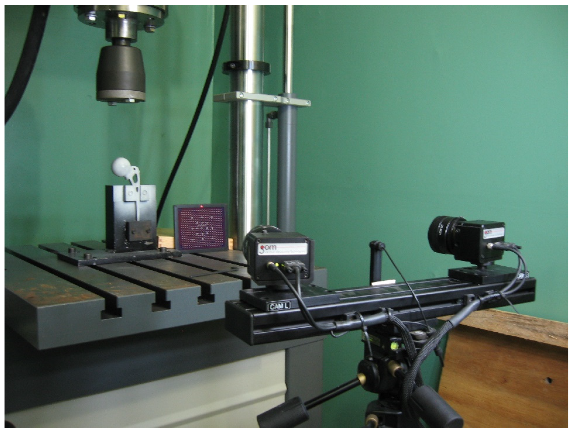
Digital image correlation (DIC) is an optical, non-contact method for measuring displacement fields and deformations on a sample surface by comparing images of the sample surface in various states [16,17,18]. The reference image is taken before the start of loading, and the other states correspond to the images taken of the deformed sample. The 3D DIC method involves two cameras and stereoscopic observation to obtain a full displacement field during testing, which is schematically shown in Figure 3. By using another camera viewing the surface from a different direction, triangulation can obtain the three-dimensional coordinates of any point. Then, by comparing the differences between the initial images and the images after loading, a full three-dimensional deformation field can be recovered. In this case, software ARAMIS v6 was used for the further analysis of all experimental results, as seen in Figure 4 [35].

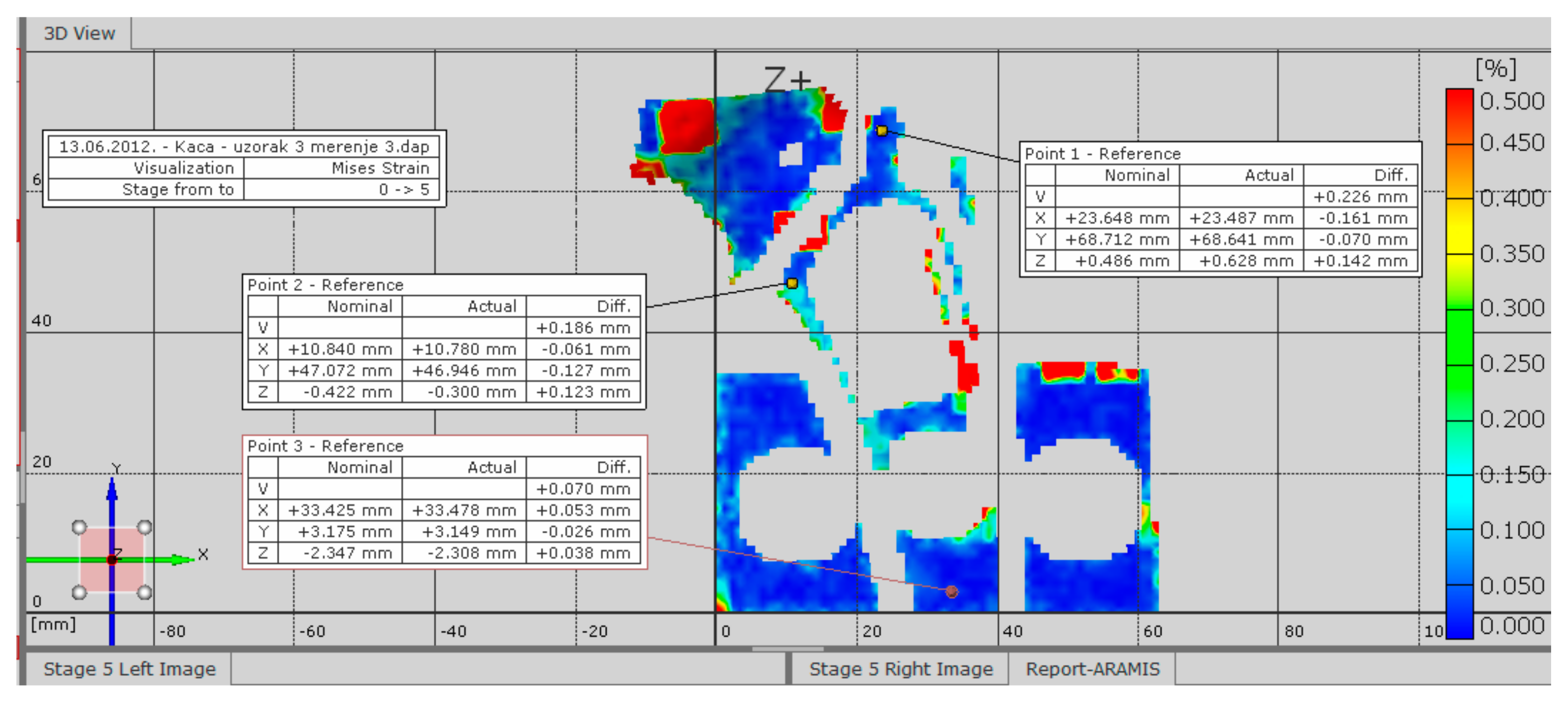
The test results for the selected sample are shown in Figure 4 for the defined measurement with an increment of −0.01 KN/s and for the selected step 5, which corresponds to a load of about 3000 N and is defined in the software for three-dimensional deformation measurement. The results show the deformation field at the moment when the load value was 3.20 kN in a step.

These diagrams show the values of deformations at the reference points, which are placed in areas of expected stress concentration due to the existence of openings on the implants, as a stress concentration factor. Reference points were chosen, allowing for a comparison between the values obtained during these experimental tests and those obtained through numerical calculations, thereby facilitating the verification of both the experimental and numerical results.

4. Numerical Models

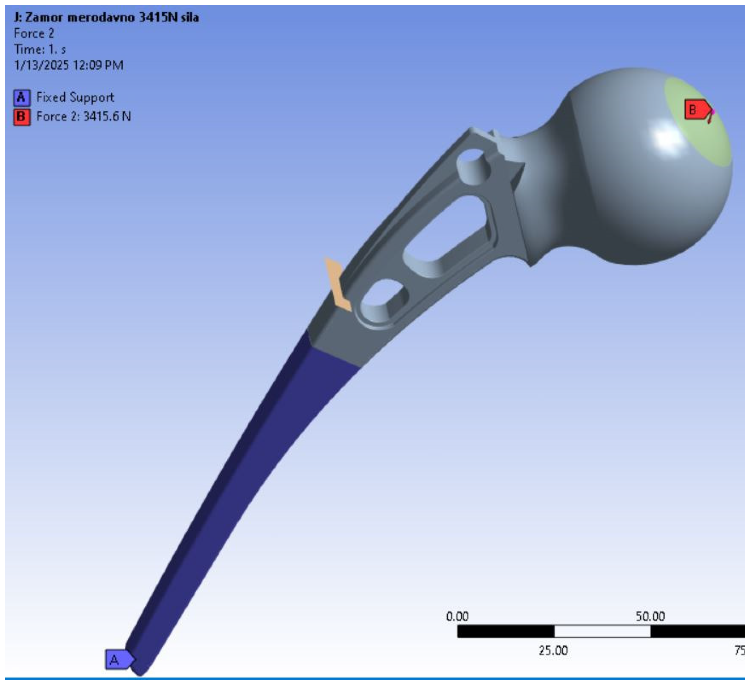
This section of the paper covers the development of a representative numerical model, using finite element software ANSYS Workbench 2022R2 version. The presented model was mainly based on the existing models used for static calculations, since the geometry, boundary conditions, and the direction of the load were the same in both cases [36]. The model geometry is shown in Figure 5, along with the load magnitude of 3415 N, since the previous analyses confirmed that this is the limit case for static loading for the geometry in question [36]. The boundary condition was selected as fixed to better represent the actual connection between the artificial hip implant and bone. As for the reason why only a part of the stem was fixed, a detailed explanation can also be found in reference [36]. The loads are calculated according to the experimental observations made by Bergman et al. [37,38] for patients of normal body weight when magnitudes and directions were selected from telemetry measurements and are given on a scale for a 65 kg person. Within the presented results, it can be seen that the case involving climbing up the stairs was the most critical one.

The location of the fatigue crack can also be seen in Figure 5, and corresponds to the part of the stem where highest tensile stresses were calculated during the previous simulation [34]. This critical location, in terms of stress, coincides with the part of the stem where the implant was fractured during the experiment [18]. The initial crack length was assumed to be 2 mm, and it was positioned through the whole thickness of the stem.

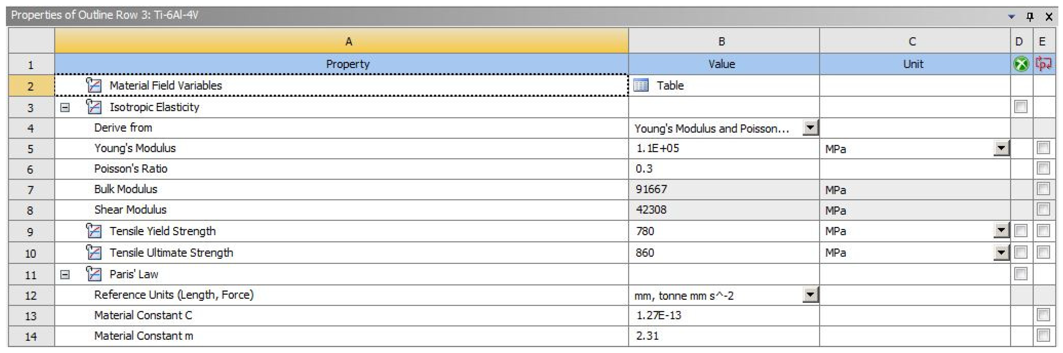
The material model used for these simulations was linear–elastic, which is commonly used for fatigue calculations. The tensile properties for the titanium alloy were determined experimentally, along with the Paris law coefficients C and m, [31] shown in Figure 6.

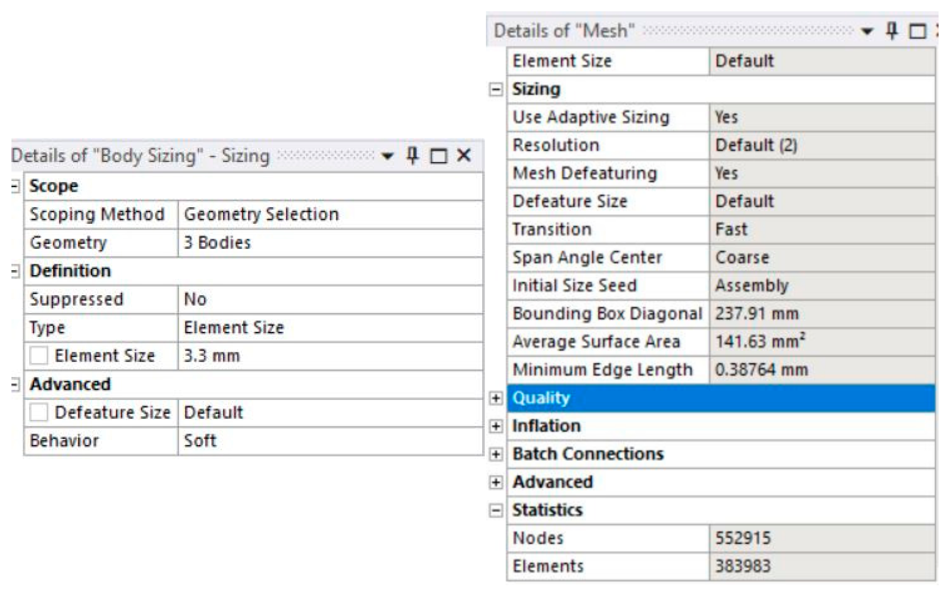
The finite element mesh is shown in Figure 7, including a detailed view of the area around the fatigue crack. Due to specific requirements imposed by ANSYS for simulations of fatigue crack growth, it was necessary to use tetrahedral finite elements, as can be seen in Figure 7. Given the geometry of the model itself, TET elements represent a better choice to begin with. Mesh was generated using the Body Sizing option in ANSYS (based on the previous experience with this option for calculations involving irregular geometries [33]), with an initial element size of 3.3 mm, as can be seen in Figure 8, with a total of 552,915 nodes and 383,983 elements. This was determined after several iterations, in order to ensure that FE size that would provide sufficient accuracy without making the calculation too long and demanding to be completed. Initial attempts were made with an element size of 2 mm, which was gradually increased in order to decrease the calculation time and determine how this affects the accuracy of the results. After an attempt with a 3.5 mm element started losing the accuracy (convergence) compared to the previous iterations, it was concluded that the 3.3 mm finite element size was optimal. This was the global element size, and the selected meshing method further refined the mesh by increasing mesh density around the critical areas (mainly in the vicinity of the crack). Similar attempts of iterative determining of convergence were made for all three models, and it was concluded that the FE size of 3.3 mm was accurate enough for all three load cases.

The same model was used for all calculations; only the load was varied in order to represent different cases. For the first two models (constant load, upstairs and downstairs case), a total of 20 load steps were defined. The number of steps, which defines the total crack growth, was defined in a way that would ensure the simulation ends when the crack reaches lengths which correspond to its critical value, i.e., when the a-N curve enters the unstable crack growth region. In both cases, this would occur after 20 steps.

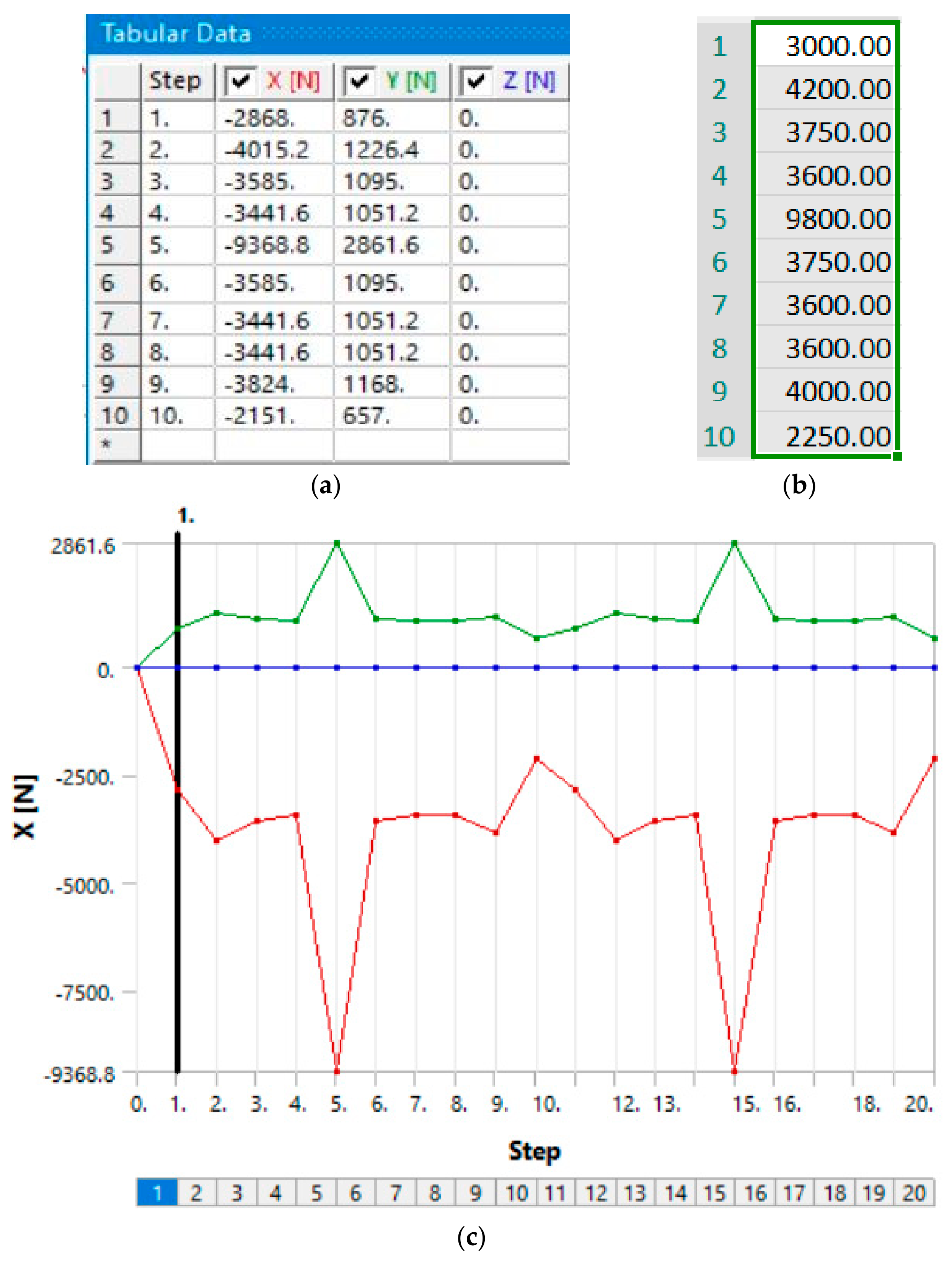
The next step in this analysis was to consider a different load case, i.e., a combination of the previous two. This simulation involved the defining of loads in a somewhat different manner, to better correspond to a real combination of different load cases. The case selected for this purpose involved going upstairs, followed by stumbling, and then going downstairs. The load spectrum was defined in accordance with standard recommendations, which can be seen in [39]. This spectrum consisted of 10 load steps, and was defined in the same way in the models. Since the previous calculations had a total of around 20 steps, it was decided to perform the combined load analysis with two iterations of 10 steps each, in order to determine if this would result in similar crack length as the first two models. Before running the 20-step model, a model with only 10 steps was made to further compare crack lengths and also as a base for verifying the bigger model by checking the results, which confirmed that the model with a load spectrum was functional, as it provided fatigue results which seemed realistic when compared to the first two models. The load, in the form of a table, is shown in Figure 9a. The table displays the axial components of each load, whereas Figure 9b shows their actual (resultant) values. Each load step had to be defined in this manner, since the direction of the force did not align with any axes, but had to be divided into directional components. Figure 9c shows an example of this load for the X-axis in the form of a diagram for all 20 steps.

5. Results and Discussion

The models presented in the previous section were simulated under the previously mentioned loads of 3415 N and 3143 N, and the results for stresses, stress intensity factors, and the number of cycles are shown in the following figures.

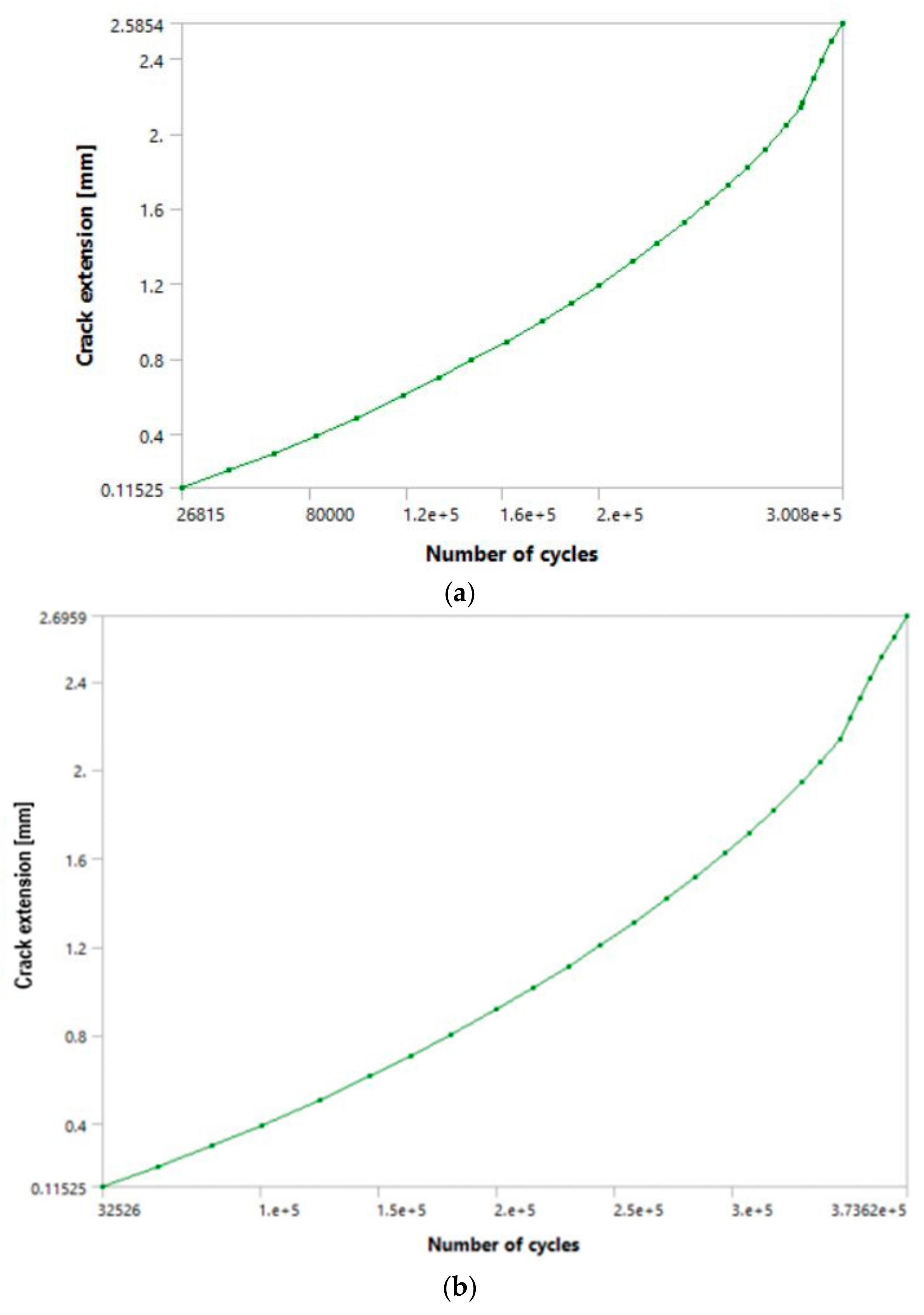
These results were achieved after a total of 19 load steps for the greater load, and 20 steps for the smaller one, since it was determined that at these points, the fatigue crack growth enters its unstable stage (as can be seen in the Figure 10a,b), and that further analyses were unnecessary. This was confirmed in the initial attempts with a higher number of load steps, which would cause the calculation to terminate due to excessive crack length.

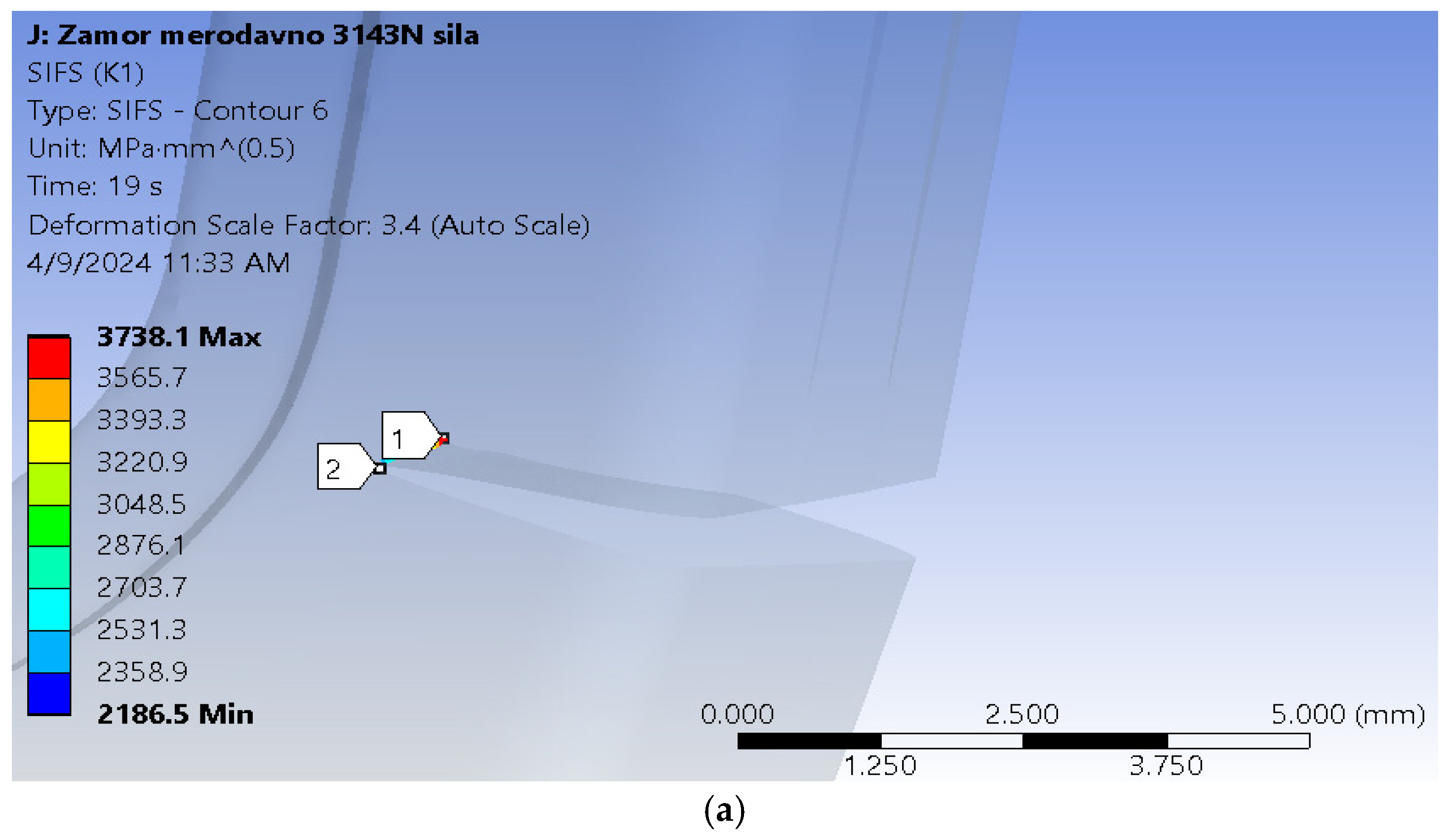
It can be seen from Figure 11 that the fatigue crack propagated through most of the hip implant stem thickness, reaching the section where the stem is narrowed in the immediate vicinity of hole.

Values of SIFs that can be seen in Figure 12 further confirm this, as their values have considerably exceeded the fracture toughness of the material in question. It should be emphasised that the values of 2.6 mm (3415 N load) and 2.7 mm (3143 N load) seen on the crack length axis in diagram from Figure 8 represent the crack growth, without including the initial crack length of 2 mm. Hence, the total fatigue crack length which would lead to failure caused by fatigue in this case would be 4.6 mm in the first, and 4.7 mm in the second case.

The number of cycles for the higher load was around 300,800, with the unstable crack growth stage initiating around 280,000, as can be seen by the change in slope of the diagram in Figure 11a. In the second case, with a lower magnitude load, the number of cycles was expectedly greater and was around 373,600. Unstable fatigue crack growth can be observed around the 350,000 cycle (Figure 11b).

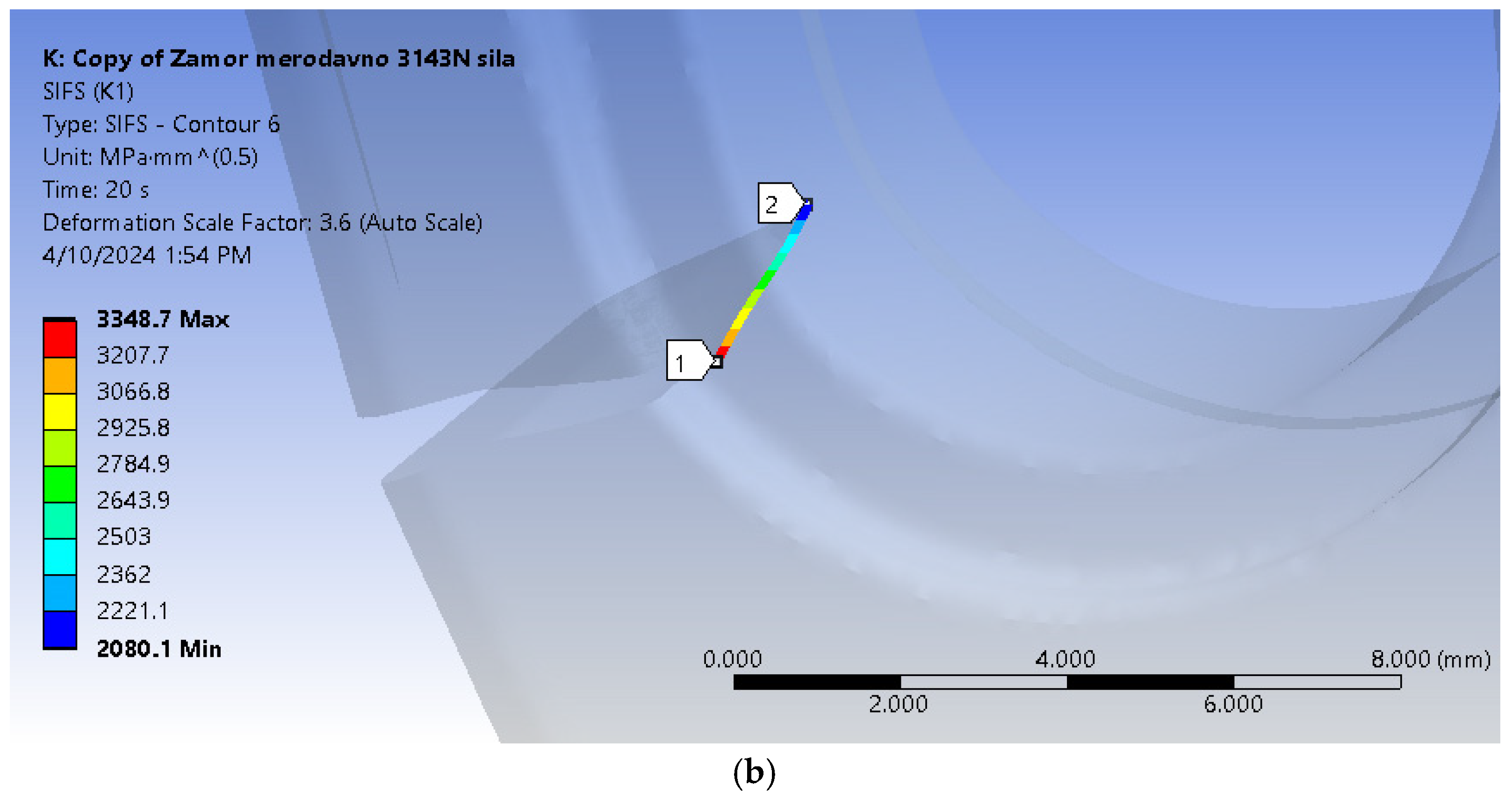
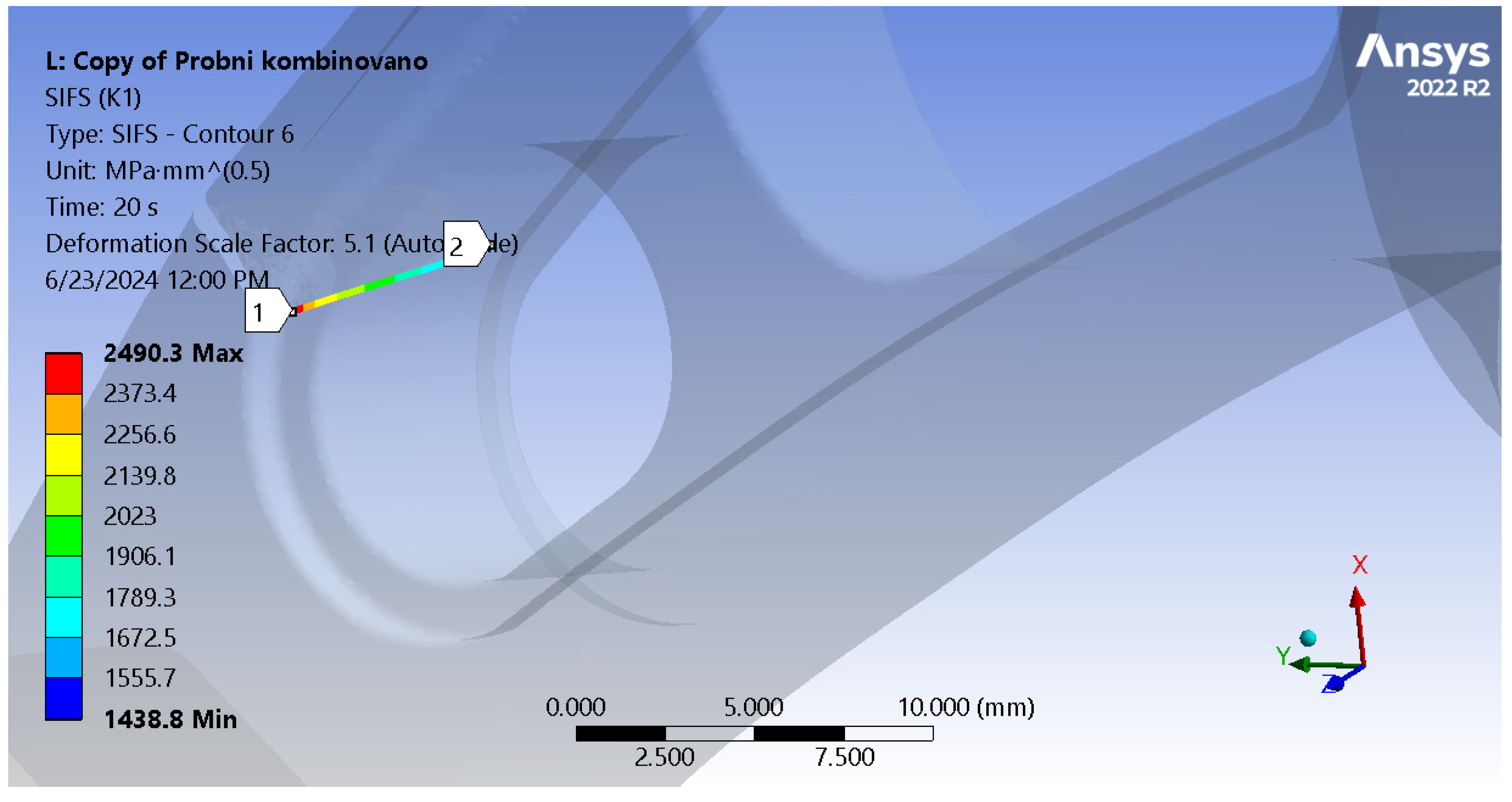
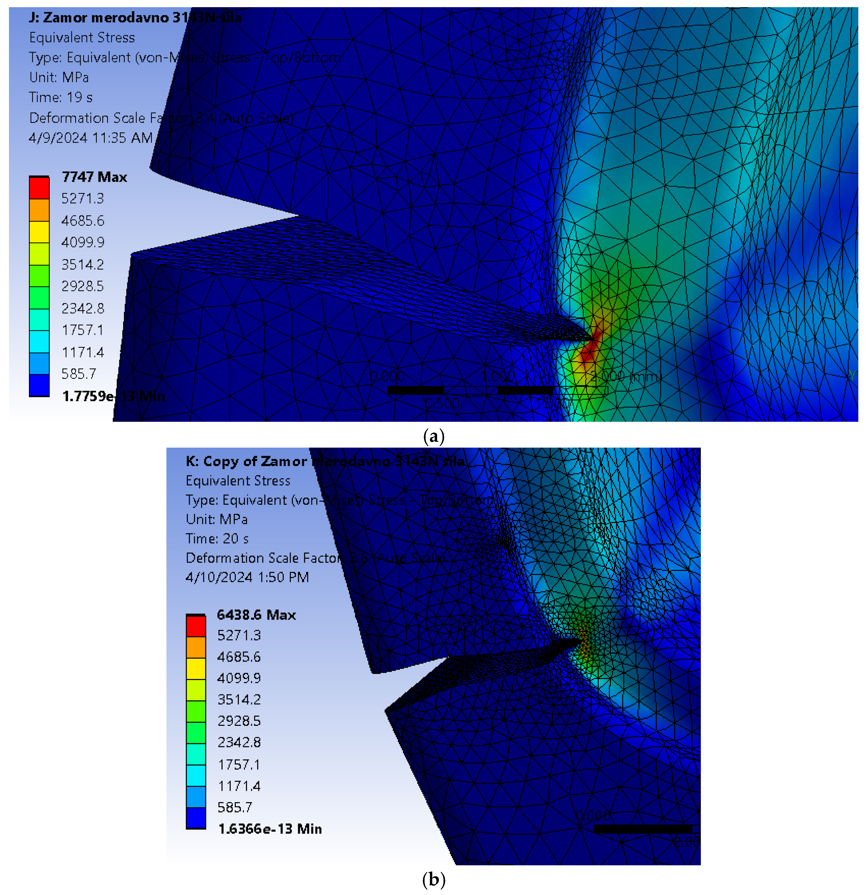
For the load spectrum, the numerical model stress intensity factors along the crack tip are shown in Figure 13, and it can be seen that they range from 1438.8 to 2490 MPa·mm^1/2, with maximum values going above the materials fracture toughness (which was determined to be around 2100 MPa·mm^1/2). Figure 14 shows the stress distribution in the model, with a more detailed view of the area around the crack tip, where stress concentration is clearly visible. Yet again, the fatigue crack propagated all the way into the thinner part of the stem, near the hole.

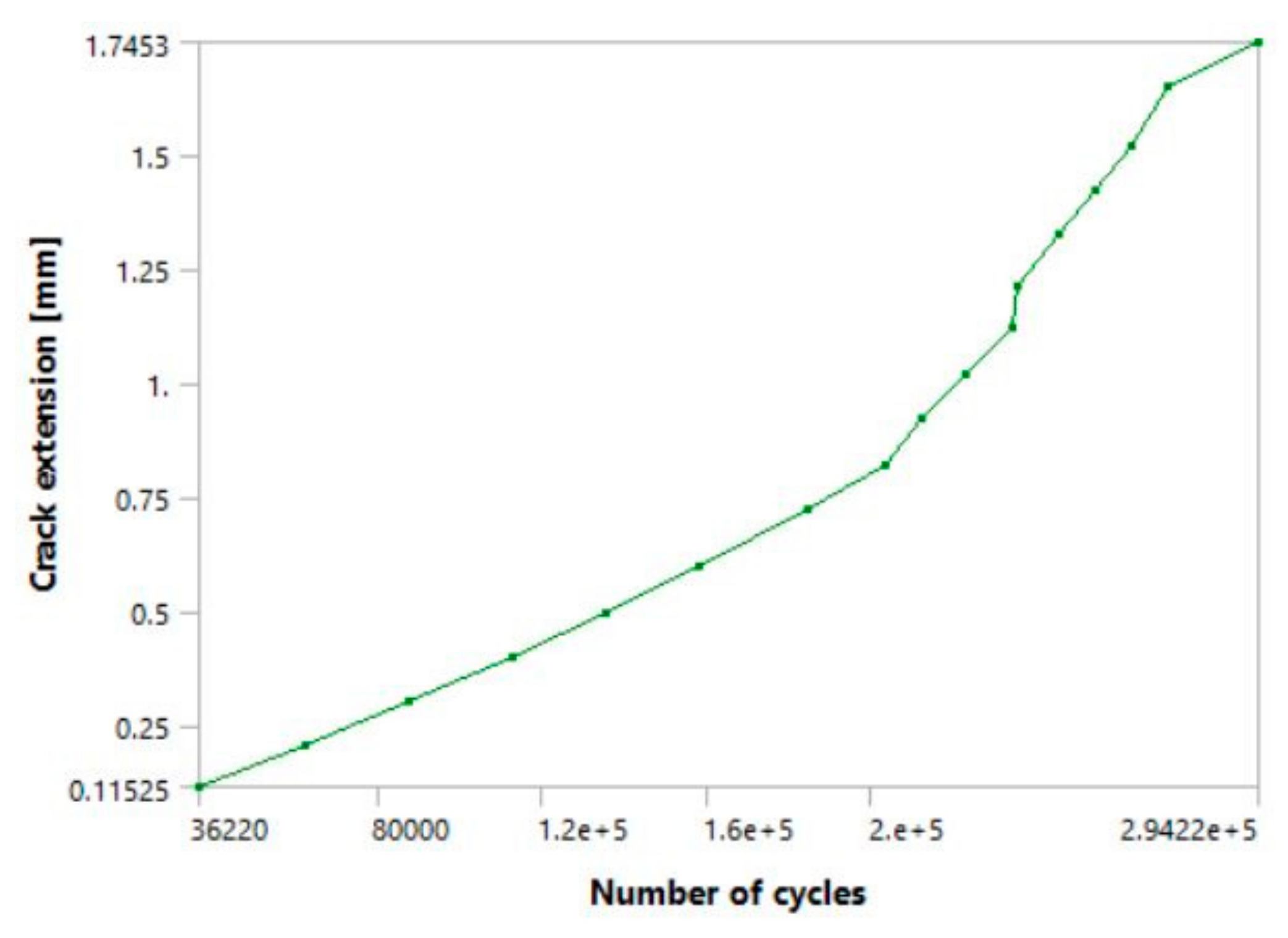
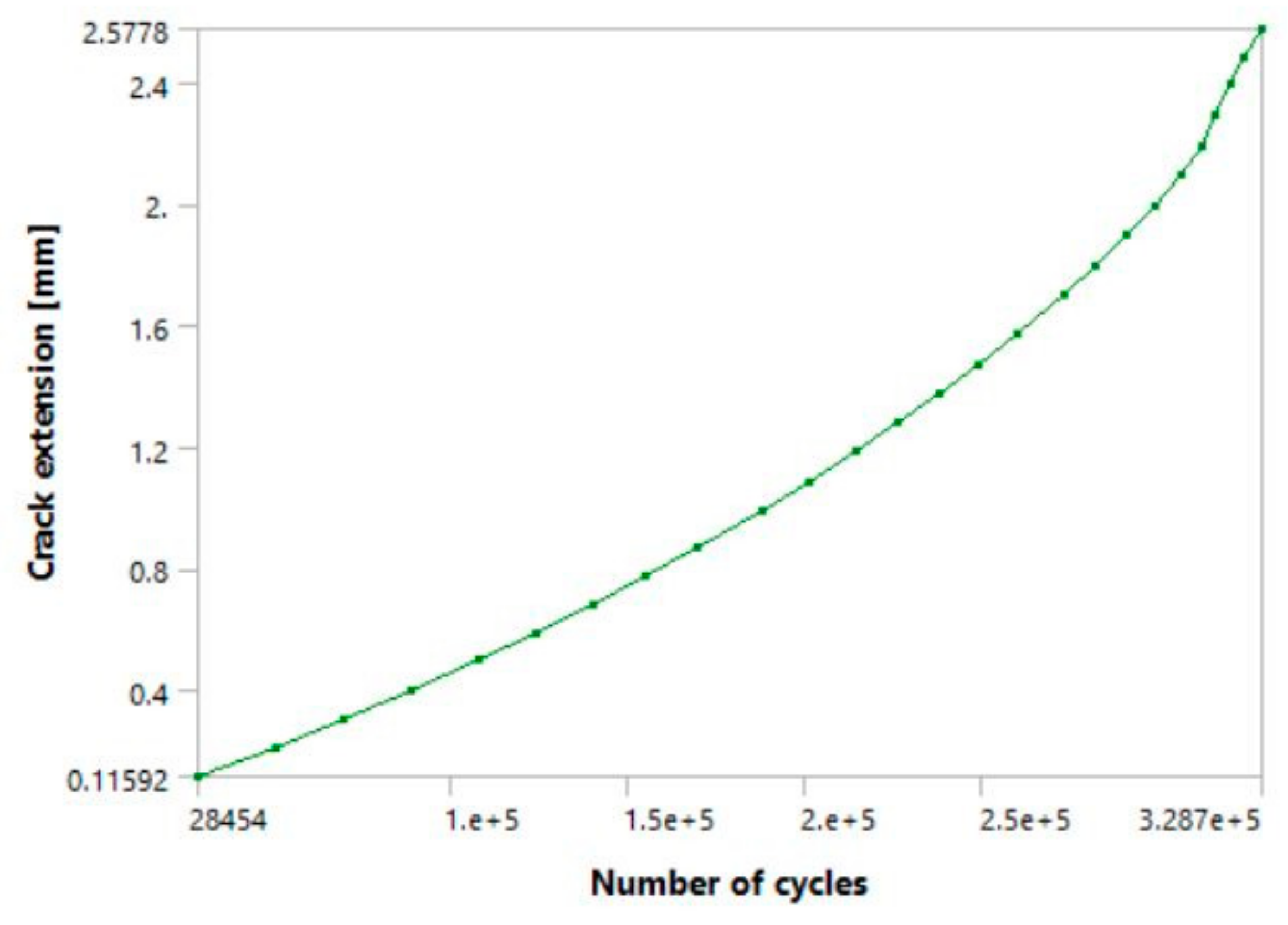
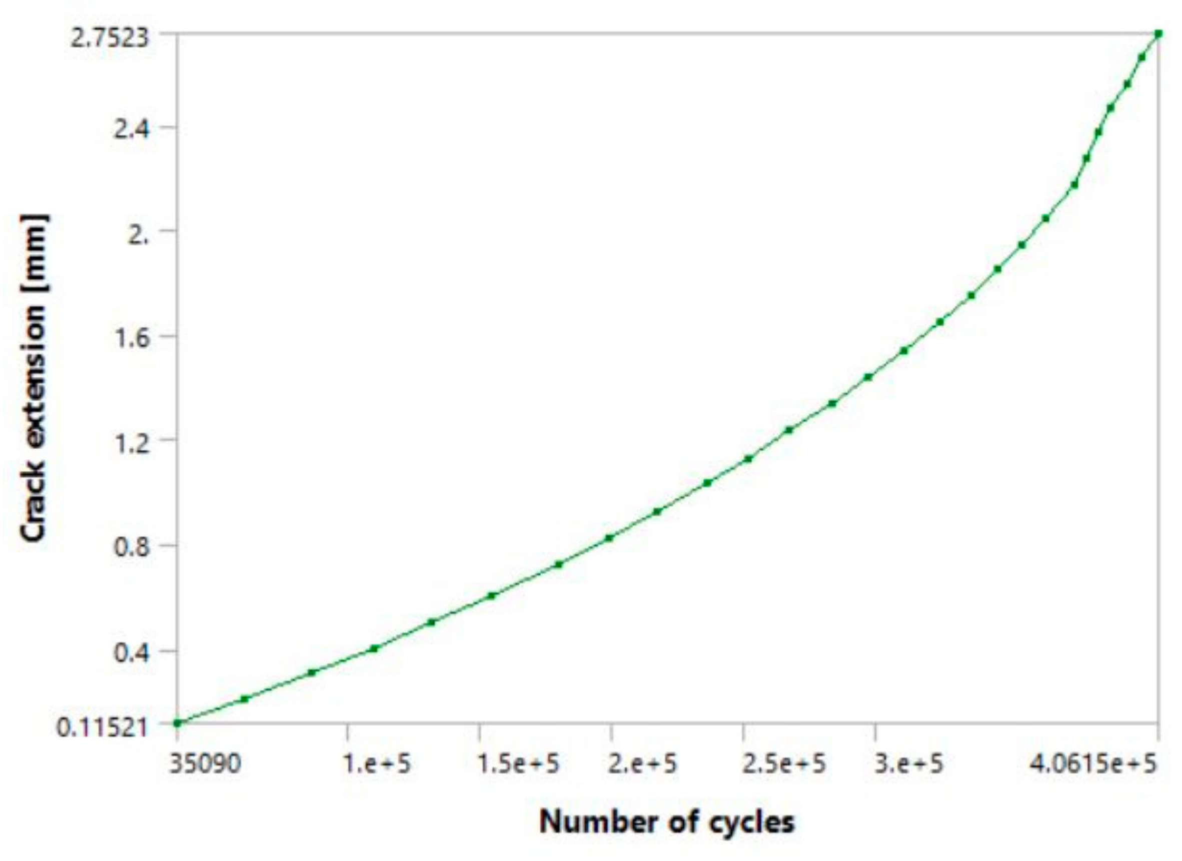
Figure 15 and Figure 16 show the a-N diagrams for 10 and 20 steps, respectively. The latter had total crack extension which was very similar to the first two models (downstairs and upstairs load cases), whereas the former had a somewhat shorter crack growth, as expected. The shapes of both diagrams are very similar, and have prominent anomalies and jumps in their curves, which was also expected in this particular case.

In addition to the results presented in the previous section, models were made with all three Paris coefficient pairs that were experimentally determined in [31], in order to determine which combination of fatigue parameters is the least favourable, i.e., which one will result in the lowest number of cycles until failure. Since it was determined that the load case with a force of 3415 N was the most critical (upstairs model), the results of these additional simulations are shown in Figure 17 and Figure 18. Based on the a-N curves from these figures, it can be seen how different Paris law coefficient combinations affect the resistance to fatigue crack growth, with the other two C and m pairs resulting in a slightly higher number of cycles. This confirmed that the selected combination of Paris coefficients (as seen in Figure 5) was indeed the most dangerous one, as it produced the lowest number of cycles.

Based on the results presented in the previous sections, certain differences can be observed, mainly in terms of the shape of the a-N curves. In the first two cases, the loads had a constant magnitude through all simulation steps, resulting in smoother curves that behaved in a way typical for fatigue simulations. In the third case, however, the situation changed due to the use of a load spectrum; the changes in the slope of the a-N curve are clearly visible in Figure 14 and Figure 15, along with occasional sudden jumps in crack extension/length, all of which can be seen while the fatigue crack is still in its stable growth stage. In the case of the 10-step model (one full load spectrum), it took the crack a total of around 294,220 cycles to reach a total crack extension of ~1.75 mm. In comparison, the 20-step model had a total of 339,410 cycles and crack extension of about 2.6 mm, almost identical to the first two models. Its unstable crack growth stage initiated a bit after the tenth step, somewhere around the 300,000 cycles. This suggests that the main difference between the two models is that the model with 10 load steps remained in the stable crack growth area, while its transition into the unstable region occurred almost immediately after the tenth step. This is supported by the fact that the total difference in cycles is only around 47,000 (approximately 14%), despite the total number of load steps being doubled, or increased by 100%.

Regarding the crack length at failure, it was very close to 3.6 mm in all three cases (including the 1 mm initial length and 2.6 mm extension during the simulations), regardless of how the load was defined. The fact that the fatigue crack progressed almost all the way through the hip implant stem before reaching its critical value suggests that the selected material demonstrates good resistance to fatigue crack growth. Although these crack lengths seem small, the number of cycles to failure is still very high, especially considering that these models were made with more extreme load cases, assuming constant walking up and/or down stairs. Additionally, the results in question were obtained for models with an initial crack, which implies that the fatigue life of undamaged implants would be even greater. The cycle numbers obtained through this analysis imply a fatigue life of at least 3–4 years under aforementioned extreme conditions. This is one of the main reasons why this titanium alloy is widely used in the manufacturing of implants subjected to such loads during their use.

Further validation of the results obtained here can be seen when comparing them to the results obtained by experiments and numerical simulations from [27]. This research involved the same titanium alloy, and was also related to hip implants. While the number of cycles did differ by order of magnitude (10⁶ in [31] vs. 10⁵ [31]), this can be easily explained by the fact that the other model had a fatigue crack in the neck, rather than the stem (thus having a significantly larger load-bearing cross-section), and that its own stem was not weakened by the presence of holes, as was the case presented here. Hence, the results of both types of simulation make sense when compared to each other, as well as the experiment from [31] which showed very good agreement with the numerical simulations.

As it can be seen from comparing the total number of cycles, the combined load case falls between the upstairs load case and the downstairs load case, having a fatigue life which is around 13% higher than the upstairs model (3415 N load). The downstairs load model resulted in around 10% more fatigue cycles until failure compared to the combined load. Potential explanation lies in the fact that some individual steps in the combined load model were actually lower than the constant loads in the upstairs model (the first and the final step). This resulted in the a-N curve having a smaller slope at the beginning of the combined loading, which led to a slower initial crack growth rate, as seen in the corresponding diagrams. It should be noted that these results are currently limited to a small number of analysed cases, and further verification is planned through thorough numerical and experimental investigations, which will also include statistical analysis.

6. Conclusions

The research presented in this paper involved the application of numerical simulations to analyse the integrity of artificial hip implants under fatigue loading. Based on the presented results, the following conclusions can be drawn:

• The use of numerical methods, mainly based on FEM, enabled the performing of analyses of the mechanical behaviour of implants under fatigue loading for several different load cases, without the need for extensive clinical tests, while also decreasing the need for experiments. This is one of the main benefits of the work presented here, reflected in increased efficiency of analysing the issue of fatigue failure of orthopaedic hip implants.
• It was determined that a novel combined approach using experimental and numerical methods represents an effective means of analysing the behaviour of hip implant under fatigue, with the main focus on crack growth and remaining life of such structures. The comparison of experimental and DIC data with numerically obtained results confirmed the validity of this approach.
• The results obtained this way can be effectively used for predicting the possibility of Ti-6Al-4V implant failure under variable cyclic loads, in cases where fatigue cracks have initiated in the implant, with varying crack lengths and positions, with the latter being defined in accordance with critical stress concentration locations, which, in turn, depend on the load type and geometry.
• The influence of different Paris coefficient pairs, experimentally obtained for the same material on numerical results was further analysed in order to confirm which combination is the most critical one, thus providing a quick and effective way of choosing the most representative combination. Hence, this represents another novel contribution of this work.
• The results for fatigue life of an artificial hip implant subjected to different load cases have indicated that there are significant differences in its behaviour, thus pointing out the importance of analysing every case individually since these loads are influenced by specific activities of each patient. The presented results have revealed that walking up stairs decreases the fatigue life of hip implants by around 25% compared to walking down stairs (373,000 vs. 300,000 total cycles), whereas the combination of both loads is almost halfway between them. Considering the average activity of these patients and how often they are likely to use the stairs, this could result in fatigue lives of up to 10 years.
• Finally, the methodology shown in this paper can be applied to other implants with different geometries, and other biomaterials. The next steps in the development of this methodology will involve numerical simulations of different load cases for varying body weights in order to obtain a more detailed insight into the behaviour of artificial hip implants under fatigue loading. It could also include a more probabilistic approach, as future work will involve many more models, as well as various load/material/geometry combinations.