Article

Predicting Fatigue Life of 51CrV4 Steel Parabolic Leaf Springs Manufactured by Hot-Forming and Heat Treatment: A Mean Stress Probabilistic Modeling Approach

by
Vítor M. G. Gomes
1,2,*,
Miguel A. V. de Figueiredo
1,
José A. F. O. Correia
1,2,3 and
Abílio M. P. de Jesus
1,2
1
FEUP, Faculty of Engineering of the University of Porto, 4150-564 Porto, Portugal
2
INEGI, Institute of Science and Innovation in Mechanical and Industrial Engineering, 4150-564 Porto, Portugal
3
ICS, Institute for Sustainable Construction, 4150-564 Porto, Portugal
*
Author to whom correspondence should be addressed.
Metals 2025, 15(3), 315; https://doi.org/10.3390/met15030315
Submission received: 14 February 2025 / Revised: 5 March 2025 / Accepted: 7 March 2025 / Published: 13 March 2025
(This article belongs to the Special Issue Numerical and Experimental Advances in Metal Processing)

Abstract

:
The longevity of railway vehicles is an important factor in their mechanical and structural design. Fatigue is a major issue that affects the durability of railway components, and, therefore, knowledge of the fatigue resistance characteristics of critical components, such as leaf springs, must be extensively investigated. This research covers the fatigue resistance of 51CrV4 steel under bending and axial tension, for distinct stress ratios, in the low-cycle fatigue regime (LCF), high-cycle fatigue regime (HCF), and very high-cycle fatigue regime (VHCF) using experimental data collected in this work and from previous experiments. Two fatigue models were analyzed: the Walker model (WSN) and the Castillo–Fernández–Cantelli model, CFC, adapted for the presence of mean stress (ACFC). According to the analysis carried out, both fatigue resistance prediction models provided good results for the experimental data, with the ACFC model showing good fitting when considering all the failure data and outliers. Additionally, fracture surfaces showed a higher trend for crack initiation on the surface for positive stress ratios despite internal defects also possibly being responsible for some fatigue failures. This investigation aimed to provide a probabilistic fatigue model encompassing the LCF, HCF, and VHCF fatigue regimes for distinct stress ratios for the fatigue design analysis of 51CrV4 steel parabolic leaf springs manufactured by hot-forming processes with subsequent heat treatments.

1. Introduction

1.1. The Manufacturing Process of Parabolic Leaf Springs

In railway vehicle design, the maximum longevity of their components must always be considered. Their essential elements for the operation and safety of the railway vehicle must also be designed to operate for several years, with only inspection and repair operations being necessary [1]. Railway components such as wheels, axles, bogies, and leaf springs (see Figure 1) are some of the rail components developed to operate for a large number of cycles [2,3,4].
Leaf springs are subjected to various forming procedures to obtain their required high mechanical characteristics. The blooms, billets, or ingots are hot-worked to obtain high quality, eliminate some internal defects or non-metallic inclusions, and finally obtain the desired cross-section and flat length for leaf springs [5]. The obtained flat leaf is re-heated in a heating furnace up to the formability temperature to be able to perform the forming processes that provide the final geometry of the component. The most common hot-forming processes for spring leaves are tapering using forging systems of mobile-fixed rolls, folding, drilling, and cutting (front and rear eyes, C shapes, etc). The leaves are then quenched and tempered with the specified camber in a press-break machine. Then, procedures to improve the mechanical characteristics, such as shot-peening, are carried out to increase the fatigue resistance on the surface before its assembly [6,7].
Figure 1. Illustration of parabolic leaf springs in a freight wagon bogie suspension. Adapted from [8], with permission from Pixabay, 2024.
Metals 15 00315 g001

1.2. Mean Stress Effect in Metallic Materials

Regarding suspension leaf springs, these are subject to cyclic loading with non-zero mean stress due to the weight of the vehicle and the payload to be transported. This load spectrum is common in vehicles’ suspension springs. In the specific case of leaf spring suspensions, the stress ratio, R, is usually quite high, which may be greater than 0.7 due to the high ratio between the sustaining load and the amplitude of oscillation (resulting from the roughness and variability in the track geometry [9]). Knowing the detrimental effect of mean stress on the fatigue life of metals [6,10,11], fatigue prediction models that measure the effect of mean stress should be considered for correct prediction of the fatigue life of leaf springs.
Several fatigue prediction models have been created to model fatigue resistance under the effect of mean stress. Classical models based on a stress approach, such as Soderberg, Goodman, Gerber, and Morrow, are models that present a fatigue strength relationship between monotonic strength properties, mean stress, and applied stress amplitude [6]. According to the Soderberg, Goodman, and Morrow models, compressive stresses do not have a negative impact on fatigue strength for long lives. In contrast, fatigue strength can be increased for steels and aluminum [12,13]. In parallel, other representations were developed, such as the example of the Haigh diagram that represents various combinations between maximum and minimum stress levels for constant fatigue lives [14].
Later, other models contemplating the mean stress effect, from the calculation of reference stress, σ a , r , as a function of the number cycles for fatigue failure, N f , emerged. Among these models, the Morrow model stands out, which is a modification of Basquin’s model, as well as Walker’s model, where σ a , r is given for a stress ratio, R, and a fitting parameter, γ , which can be linearly related to the maximum applied stress for some materials [15,16]. This parameter can be seen as a sensitivity parameter of the material to the presence of mean stress, ranging from 0 for insensitive to 1.0 for fully sensitive to mean stress. The Smith, Watson, and Topper model is a particularity of the Walker model, where the fitting parameter γ = 0.5 [17]; however, in accordance with previous investigations, the Walker method provides better predictions for estimating the parameter γ [16,18,19,20]. The Walker model provides more conservative results for cases of higher mean stress in the low-stress range zone and non-conservative results for regions of higher stress for some materials [16]. Later, Kwofie suggested a correction in the fatigue model due to mean stress [21,22], which is represented by the parameter designated as the exponential form for the fully equivalent stress amplitude, EFRSA, whose sensitivity to the presence of mean stress is quantified by the coefficient α k , with the value of α k = 2.0, indicating that the material exhibits great sensitivity to the presence of mean stresses [21].
For models considering local strains, the Coffin–Manson and Basquin prediction model, CMB, has been the basis for the development of new prediction models accounting for the mean stress effect. The CMB model is primarily used when the strain magnitude level is higher than the yield strength of the material (low cycle fatigue, LCF); however, the CMB model can also be used for high-cycle fatigue, HCF, regions. Some widely employed fatigue models that consider the mean stress effect following a strain-life approach are the Morrow model [23]; the Manson and Halford model [24]; and the SWT model [17], where this has the disadvantage of being only applied to non-zero mean stresses. In contrast, the SWT model has provided better agreement for a wider range of materials [14] than the Morrow and Manson and Halford fatigue models. Another strain-life fatigue model suggested by Ince and Glinka [25,26] relates the generalized strain amplitude parameter, GSA, with the fatigue life. According to these authors, the mean stress effect is better correlated to the fatigue life if only the component of the elastic strain amplitude is affected, in contrast to the SWT model. Similar to the stress-life approach, Walker also generalizes the SWT model for a strain-life approach using a fitting exponent termed as γ [27,28]. Subsequently, the Walker model was refitted to the Dowling model, with fitting parameter γ w [29]. According to [16,18], the higher the value of γ w , the lower the sensitivity of the material to the stress medium and vice versa, which is the opposite of the Walker parameter such that γ = 1 γ w [30].

1.3. Article Outline

In this paper, fatigue resistance analysis methodologies for steels are applied to evaluate the mean stress effect on 51CrV4 steel, widely applied in both rail and road vehicles. Probabilistic fatigue analyses based on failure probability curves for Gaussian and Weibull distributions are considered.
Since leaf springs operate under bending loads, the samples should be tested under similar loading conditions. To adhere to this requirement, three-point plane-bending fatigue tests in a home-made machine for a maximum lifetime of 5 × 10 6 cycles are carried out. For a better representation of the behavior under the influence of mean stress, the failure data obtained in the analysis performed in [31], rotating bending failure data (at R σ = 1 ), are considered in this analysis. According to several studies carried out, the mechanical behavior of leaf springs can be evaluated using some theoretical models, the cantilever beam model [32] and the four-point in-plane bending model [33], but also in three-point bending models [33]. In [34], the effect of boundary conditions was numerically evaluated using the finite element method, showing that the rotating bending test yields a lower fatigue strength than the cantilever and four-point bending tests; however, this reduction is much higher in the low-cycle fatigue regime, LCF, with our bending failure data tested in the high-cycle fatigue, HCF, regime, and in the very high-cycle fatigue regime, VHCF, being able to be combined.
Additionally, following the same assumption in [31], axial tension fatigue tests for positive R σ are also performed (up to 3 × 10 6 cycles) and combined with the fatigue failure data presented in [31,35] regarding axial tension/compression with a maximum lifetime of 10 9 cycles. This analysis allows us to obtain the fatigue resistance with and without the existence of mean stress, not only for the high-cycle fatigue, HCF, regime but also for shorter lives in the low-cycle fatigue (LCF) regime and for very long lives in the very high-cycle fatigue (VHCF) regime. The sensitivity to the presence of mean stress for each type of loading (separate and combined) is analyzed using the Walker SN model (WSN). Considering a large amount of data in the fatigue limit zone, a large number of outliers (failures and run-outs), and the good representation that the Castillo–Fernández–Cantelli, CFC, model has proved for the regimes of LCF, HCF, and VHCF, the CFC fatigue model with a Weibull distribution, adapted for the existence of mean stress, is also evaluated.
The fracture surfaces obtained in the experimental campaign of three-point plane bending and uniaxial tension fatigue tests are analyzed using scanning electron microscopy, SEM, and compared with the fracture surface analysis performed in [31]. The fracture surface analysis allowed us to observe that, for positive stress ranges, fatigue fractures begin essentially on the surfaces of specimens; however, initiation from non-metallic inclusions may also occur.
As a result of the research carried out in this article, a probabilistic fatigue prediction curve based on the CFC model with prediction of the mean stress effect, encompassing the LCF, HCF, and VHCF fatigue regimes under normal stress amplitude conditions (bending, uniaxial, or combined), is suggested. The suggested fatigue model was developed with 51CrV4 steel data obtained from parabolic leaf springs subjected to a heat treatment of quenching and tempering and the hot-forming process. Despite this particularity, this model can be used in other components composed of 51CrV4 that guarantee the same type of heat treatment.

2. Fatigue Modeling

2.1. Walker SN Fatigue Model

One of the most useful methods for the prediction of fatigue resistance and commonly applied in fatigue design codes [36] is the use of SN curves, which relates the stress amplitude level, σ a , with the number of cycles to failure, N f , based on an average curve. Log–log straight-line SN model suggested by Basquin [37,38] is one of the most applicable methods for predicting the fatigue life. For a certain stress ratio, R σ , the Basquin fatigue model is written as
σ a = Δ σ 2 = C b N f n b ,
with Δ σ denoting the applied stress range, C b the strength coefficient, and n b the strength exponent.To contemplate the stress ratio effect, a reference stress amplitude, σ a , r , determined by Walker model can be assumed. According to Walker model [15], the reference stress amplitude is given as
σ a , r = σ m a x 1 γ σ a γ = σ m a x 1 R σ 2 γ = σ a 2 1 R σ γ ,
with σ m a x denoting the maximum stress applied and γ denoting a material parameter that can be fitted by dataset optimization/fitting methods. Thus, the Walker model is written as
σ a , r = σ a 2 1 R σ γ = C b N f n b .
According to previous investigations, the Walker method (Equation (3)) provides better predictions for estimating the parameter γ [16,18,19,20]. If γ assumes the value 0.5, σ a , r in Equation (2) is σ m a x σ a , which is the reference stress given by Smith, Watson, and Topper, SWT, model [17]. For some materials, γ parameter can be dependent on σ m a x applied at the cycle. A linear relationship between the log σ m a x and the parameter γ was deduced in [16], having presented a better fitting than the equation model (2). Thus, the parameter γ of Equation (2) can be written as
γ = γ 0 + γ 1 log σ m a x ,
and hence Equation (3) is rewritten as
σ a , r = σ a 2 1 R σ γ 0 + γ 1 log σ m a x = C b N f n b ,
where γ 0 and γ 1 are parameters being determined along with Equation (2).
The determination of parameters, C b , n b , γ 0 , and γ 1 is performed according to the ordinary least-squares method, OLS, for a linearized model of Equation (5), with the independent variables given by log ( σ a , i ) , log 2 / 1 R σ , and log σ m a x log 2 / 1 R σ and the dependent variable given by log ( N f , i ) , with i denoting the respective data point [16] such that
log ( N f ) = β 0 + β 1 log ( σ a ) + β 2 log 2 1 R σ + β 3 log σ m a x log 2 1 R σ ,
with β 0 = log ( C b ) / n b , β 1 = 1 / n b , β 2 = γ 0 / n b , and β 3 = γ 1 / n b . Notice that, when γ is constant with σ m a x , γ 1 = 0 , and hence β 3 = 0 . Thus, Equation (6) is rewritten as
log ( N f ) = β 0 + β 1 log ( σ a ) + β 2 log 2 1 R σ .
Equations (6) and (7) are solved using multi-linear regression methods [39]. Notice that Equation (7) is in accordance with the standardized procedure in ASTM E732-9 standard [40] if the mean stress effect is not considered.
According to the linear regression model, the points around the average curve are assumed to have a Gaussian probability distribution function with the failure probability, P f , defined as
P f = 1 2 1 + erf N f β 0 + i = 1 3 β i μ σ a , i 2 σ N f ,
where erf · denotes the error function, μ σ a , i denotes the average value of the independent variables, and σ N f denotes the standard deviation of the dependent variable. Notice that, in the WSN fatigue model presented here, run-outs are not considered in the definition of the failure probability function.

2.2. Apetre and Castillo–Fernández–Cantelli Fatigue Model

The Castillo–Fernández–Cantelli, CFC, fatigue model can be taken into consideration for a more accurate representation of fatigue behavior. CFC fatigue model takes into account statistical requirements for fatigue representation such as the weakest link principle, stability, a limited range, limit behavior, and the satisfaction of the physical conditions. CFC fatigue model has the advantage of being applicable for representation of the fatigue strength from low- to high-cycle fatigue regimes, and even up to a very high-cycle regime. Following the limit behavior and the limit range assumptions, random variables following a statistical distribution of extreme values are recommended. Weibull model has been considered for modeling the fatigue failure probability for medium, long, and even very long lives instead of Gumbel model [31,41,42,43,44,45,46,47].
For a stress range given life or vice versa, the failure probability, P f , for CFC model following a Weibull distribution [38,48,49] is
P f = 1 exp V λ δ β ,
where V denotes the Weibull random variable, which is given as
V = log N f B log Δ σ C ,
which implies that log N f B log Δ σ C λ .
In Equation (9) λ , β , and δ are the location, the shape, and the scale parameters of Weibull’s distribution, respectively, whereas, in Equation (10), the fatigue life, N f , the stress range applied, Δ σ , the logarithm of the threshold value for life N f , denoted as B, and the logarithm of the threshold of the fatigue life for a fatigue limit, σ f , denoted by letter C. log N f = B and log Δ σ = C represent, respectively, the asymptotes of a hyperbolic function. log Δ σ = C may be associated with the fatigue limit, which, in case of materials not exhibiting a fatigue limit, C is equal to 0. This model has proven good agreement with several fatigue life analyses [38,50,51,52,53].
Equation (9) assumes that the loading is fully reversible (null mean stress); however, this limitation is overcome by replacing Δ σ , for a fatigue parameter, ψ i , with index i indicating the type of quantity to be considered. Fatigue parameters suitable for ψ i can be given by SWT, Walker model, and others [29]. Apetre et al. [54] proposed the Walker model in the form of strains, as suggested by Dowling model [29]. Thus, considering the strain fatigue parameter, ψ ε , as
ψ ε = ε a 2 1 R 1 γ w ,
with γ w the Walker parameter fitted from Dowling’s model, the Apetre and Castillo–Fernández–Cantelli (ACFC) fatigue model is written as
ψ ε = ε a 2 1 R 1 γ w = exp α 1 + λ + δ log 1 P f 1 / β log N f α 2 .
Note that the model is applicable for low-cycle, high-cycle, and very high-cycle fatigue since the fatigue parameter of Equation (11) is determined by a model that takes into account the effects of elastic and plastic deformations. Equation (12) is then related to Equation (9), resulting in
P f = 1 exp log N f B log ψ ε C λ δ β ,
after some arithmetic operations, with α 1 = B and α 2 = C . Previous knowledge of the Walker parameter, γ w , allows the determination of the probabilistic model parameters, B, C, and Weibull parameters ( β , λ , and δ ) via E–M algorithm methodology [38,55]. In contrast to the WSN fatigue model, in ACFC fatigue model, run-outs can provide a certain amount of contribution to the definition of the failure probability function [38].

3. Materials and Experimental Procedure

The fatigue strength of chromium–vanadium steel for parabolic leaf springs was evaluated for three-point bending and uniaxial tensile loading for positive stress ratios and different stress levels. The region of interest for the investigation corresponded to the high-cycle fatigue regime, HCF, which comprised the region within the fatigue life corresponding to the maximum stress of material’s yield limit and the fatigue life of 5 × 10⁶ and 3 × 10⁶ cycles, respectively, for three-point bending and uniaxial tension loads. In order to analyze the stress ratio effect and extend the fatigue strength curve from the low-cycle fatigue regime, LCF, (≈103 cycles) to the very high-cycle fatigue regime, VHCF, (≈109 cycles), the fatigue failure data of 51CrV4 steel in the literature [31,35] were considered.
Initially, the failure data were combined with the data in [31,35] to evaluate the mean stress effect under different types of loading. Then, all failure data were combined into a single probabilistic field using the WSN and ACFC fatigue model approaches to determine the failure probability curves. Some of the fatigue fracture surfaces that characterise the test loading type and load level, using scanning electron microscopy, SEM (JEOL JSM 6301F/Ozford INCA Energy 350 and FEI Quanta 400 FEG ESEM/EDAX Genesis X4M), were observed to understand the fatigue results obtained. The surface quality of the specimen was verified using the Mitutoyo Surftest SJ-210 device that follows the standard Surface Texture Profile Method [56].

3.1. Materials, Microstructure, and Chemical Properties

The steel under investigation is a standardized martensitic steel quenched at 850 °C (40 min) in an oil bath and then tempered at 450 °C for 90 min, according to UIC 517-2017 [57] and ISO 6892-1 [58] standards. The 51CrV4 steel (as received) exhibits a tempered martensite structure as shown in Figure 2 [31,35,59].
In chemical terms, 51CrV4 is a medium carbon alloyed steel, with an average carbon content ≈ 0.50% with alloying elements of chromium between 0.90 and 1.20 % and vanadium between 0.10 and 0.25%. Table 1 presents the chemical composition for standardized 51CrV4 steel grades in % wt.
In terms of the mechanical strength under monotonic loading conditions, 51CrV4 steel following the ISO 6892-1 [58] standard has a modulus of elasticity, E, of 200.54 MPa, offering high mechanical strength, with the yield strength, σ y , of 1271.48 MPa and the tensile strength, σ u t s , of 1438.5 MPa, but a low ductility with a percentage elongation after fracture, ε f , of 7.53% and percentage reduction of area, R A f , of 34.69% (see Table 2) [35].

3.2. Specimen Geometry and Fatigue Testing Setup

Fatigue tests under in-plane bending conditions were performed under displacement-controlled conditions on an electro-mechanical three-point bending testing machine constituted by electric motor with a rotation speed of 1385 rpm, allowing frequencies for fatigue tests at 23 Hz, as illustrated in Figure 3. The machine has two load cells (with a maximum load capacity of 30 kN), one on each support, which are spaced by a minimum length of 150 mm. Load cell signals are periodically recorded from a data acquisition system, SPIDER 8, and acquisition software, Catman (version 4.5) The number of cycles is recorded with a display counter up to maximum of 5 × 10 6 cycles.
As regards the test specimens used for in-plane bending fatigue tests, a constant section plate is considered, with a length of 200 mm, supported on load cells distanced 150 mm from each other. Thickness, h 0 , and width, w o , are adjusted to the test machine’s maximum load and deflection requirements. The geometry of test specimens was chosen with reference to the standard for bending tests in metallic materials [60]. Figure 4 presents the geometry of the fatigue specimens with rounded corners (Figure 4 Dt. A) for three-point in-plane bending and the surface finish after milling (Figure 4 Dt. B). On the right side of Figure 4, the dimensions for definition of the specimen geometry are illustrated. These specimens were tested for positive stress ratios, namely for R σ of 0.0, 0.1, 0.3, and 0.4. resulting in 24 specimens. Table 3 presents the average dimensions of smooth specimens used in planar bending fatigue testing according to ISO 7438 standard [60].
Fatigue tests to assess the mean stress effect in HCF fatigue regime under uniaxial tensile load were carried out under force-controlled conditions in a servo-hydraulic testing machine, MTS 868, as illustrated in Figure 5. Fatigue testing machines operate at the maximum of 3 × 10 6 cycles for several testing frequencies, not higher than 12 Hz.
Concerning fatigue test specimens, a cylindrical specimen with a constant nominal diameter section in the gauge length of 4 mm was considered. The geometry of the specimen was chosen regarding the standard for uniaxial fatigue tensile tests under force-controlled constant amplitude conditions [61]. Figure 6 presents the geometry of the smooth fatigue specimen for axial tensile alternating loading and the respective CAD model. These specimens were tested for positive stress ratios, namely for R σ of 0.1, 0.3, and 0.5, resulting in 39 specimens. Table 4 presents the main dimensions of the specimen used in the tests.

3.3. Literature Data Collection

The fatigue strength data of 51CrV4 steel for extension of the model from LCF to VHCF were obtained from the literature [35] for the LCF regime and [31] for the HCF and VHCF regimes. To analyze the fatigue behavior in LCF regime, the cyclic tests in [35] were performed in constant uniaxial strain-controlled amplitude loading conditions according to ASTM E606 standard [62] for a strain ratio, R ε = 0.0 and an average strain rate d ε /dt of 0.8 %/s (see Table A1—column 6). The cyclic tests with different strain amplitudes were conducted in an INSTRON 8801 servo-hydraulic machine with a load cell of 100 kN and a dynamic INSTRON 2620-202 clip gauge with a working range of ±2.5 mm, enabling observing the elastoplastic cyclic softening behavior and the relaxation of the mean stress of the material. For longer lifetimes, in the VHCF region, the considered fatigue tests were obtained for uniaxial tension/compression ( R σ = 1 ) tests up to ≈ 10 9 cycles. Fatigue testing was conducted using the Shimadzu USF-2000 fatigue machine that operates at a resonance frequency of 20 kHz under displacement control. Due to the frequency effect, which might affect the fatigue behavior of materials, these failure data were corrected to obtain corresponding stress amplitude levels at low frequency and then to be combined with the remaining data. The information of the estimators is in Table A1—columns 3, 4, and 5 and Table A2—columns 2 and 3.
For medium lives, in the HCF fatigue regime (approximately from 10 3 up to 10 7 cycles), uniaxial tension/compression and rotating bending tests were performed for R σ = 1 . In uniaxial tension/compression, fatigue tests were performed using the Rumul Testronic HCF machine operating under load control conditions with a 150 kN load cell, following the fatigue standard [61], whereas, for specimens tested under rotating bending, the fatigue specimens were tested in a home-made machine according to the single-point loading configurations described in the ISO 1413 standard [63] operating at a testing frequency of 25 Hz. The information of the estimators is in Table A1—columns 2 and 5 and Table A2—columns 1 and 3.

4. Results and Discussion

4.1. Data Pool

In an initial approach, fatigue failure data obtained from three-point in-plane bending and uniaxial tension tests and fatigue failure data collected in [35] and Ref. [31] are analyzed separately according to the loading type.
Figure 7 presents the failure data pool obtained from the fatigue tests under rotating and in-plane bending conditions for distinct stress ratios ( R σ of 0.0, 0.1, 0.3, and 0.4). It is verified that there is low scatter in the fatigue resistance for higher stress amplitudes and larger scatter for the lowest stress amplitude levels, even considering the mean stress effect.
Regarding the axial tension/compression ( R σ = 1 ) and tension ( R σ 0 ) fatigue loading conditions, Figure 8 presents the failure data for uniaxial tests under R σ of −1.0, 0.1, 0.3, and 0.5 in subsonic and ultrasonic conditions (covering HCF and VHCF fatigue regimes) and under R ε of 0.0 (covering LCF fatigue regime). In the latter data (referenced as “SAT-EP R = 0.0” in the legend of Figure 8), the stress amplitude is determined considering the stabilized cycle, and stress amplitudes for stabilized cycles are used to determine the actual stress ratio. Notice that, in the case where maximum mean stress relaxation occurs, R σ is 1 , whereas, in the other cases, R σ is different from 1 .
Analysing Figure 8, it can be seen that, for ratios R σ and R ε , there is a reduction trend in strength that is indicated by a downwards vertical translation of the fatigue strength curve. This vertical translation of the fatigue strength curve is higher for long lives than for short lives, as expected for steel fatigue behavior. Regarding failure data close to the run-out zone ( 3 × 10 6 and 5 × 10 6 cycles), it is observed that, for stress ratios greater than 0.1, the occurrence of run-outs increases, which makes it difficult to understand fatigue strength for stress ratios greater than 0.5.

4.2. Walker SN Fatigue Model

The effect of mean stress was evaluated considering the Walker parameter based on stresses, as presented in Equation (3), for the fatigue dataset in rotating bending and three-point in-plane bending, as shown in Figure 7, and for the axial tension failure data, as shown in Figure 8. The parameters γ , C b , and n b were found by applying the multi-linear regression method to the linearized Equation (2), which is Equation (7). In addition, the relationship of the parameter γ with the maximum applied stress (Equation (4)) was also evaluated. As always, in both situations, the parameter γ proved to be constant for the different maximum stresses analyzed due to the parameter β 3 in Equation (7) being close to zero. Figure 9 presents the result of the data obtained considering the parameters given by Equations (3) for the specimens under bending conditions (rotating bending plus three-point in-plane bending). Good agreement is demonstrated between loading testing types since, in the zones of higher scatter, between 500 and 700 MPa, failures occur with the same probability, with no outlier values in comparison with the rotating bending tests, with the greatest part of the failures for the 25th percentile curve.
Regarding the average resistance curve, a C b of 3623.26 MPa and n b of −0.1419 are obtained (only 5.54% and 3.65% different compared to the data in the Basquin SN curve obtained for rotating bending conditions in [31] (see Table A1—column 2). The value of the coefficient of determination, R 2 , was 0.5729 with a parameter γ = 0.1430. As the γ parameter assumes the meaning of the material sensitivity to the presence of mean stress, then γ = 0.1430 indicates that the material has very low sensitivity to mean stress under fatigue bending loads [18]. Despite the lower sensitivity to the mean bending stress effect observed, the low value of γ may also be influenced by the increase in the material’s fatigue resistance when the samples are evaluated under in-plane bending loading conditions compared to rotating bending [34]. Table 5 presents the summary of the results obtained by the regression and the respective statistical parameters.
On the other hand, from the results obtained for the axial tension loading, a parameter γ of 0.7758 was obtained, indicating high sensitivity to mean stress under uniaxial tension loadings. Values of γ close to unity are also found in other high-strength steels [18,19,30,64]. Figure 10 illustrates the results of the multi-linear regression with all the failure data considered under tension/compression loading. One verifies that failure data with non-null mean stress are located above the failure points with null mean stress, contrary to the fatigue bending dataset. Furthermore, it was noted that the failure data are practically normally distributed for equivalent stresses above 900 MPa, even in the LCF fatigue zone. For lower equivalent Walker stress amplitude, σ a , w , the scatter begins to be higher. The regression showed an R 2 0.68 with regression parameters of C b = 2543.30 MPa and n b = 0.0886 . The coefficients C b and n b obtained are not very different from those determined in [31], with differences of 7.97% and 1.41% for coefficient C b and exponent n b , respectively (see Table A1—column 4). Table 5 presents the results obtained by the regression and the respective statistical parameters.

4.3. ACFC Fatigue Model

The effect of mean stress was evaluated using the hyperbolic probabilistic model according to the ACFC fatigue model. The ACFC fatigue model considers the ψ ε as the fatigue damage parameter (Equation (11)). Figure 11 presents the probabilistic field with failure data, run-outs, and their estimates for rotating and three-point in-plane bending data. The Weibull distribution estimators for the dataset in Figure 7 are β = 1.23 , δ = 4.27 , and λ = 13.49 . Compared with the estimated parameters presented in Table A2, the percentage differences are significant, with 34.57% for parameter β , −9.49% for δ , and −52.26% for λ . With respect to parameters B and C, the difference is observed for the damage parameter threshold value (horizontal asymptote), with an exp ( C ) value of 0.08%, which corresponds to a difference of 37.97% in the elastic equivalent stress amplitude (162.0 MPa) when compared with the stress amplitude of 261.0 MPa presented in Table A2— column 2). The vertical asymptote, exp ( B ) , also corresponds to one cycle. When ψ ε , w reaches values greater than 0.3%, most failure data are found within the 25% and 50% percentile curves. In contrast, for ψ ε , w values less than 0.3%, the dataset is more scattered within the 1% and 75% percentile curves. Regarding the average value of the distribution, a value of 17.48 is obtained, which is higher than the median value, 16.67, as shown in Table 6.
Regarding the probabilistic field model for the data obtained by axial stress tests, Figure 12 presents the dataset obtained from a low-cycle fatigue regime up to a very high-cycle fatigue regime for a fully reversed and positive stress ratio. Regarding the probabilistic field model for the data obtained by axial stress tests, Figure 12 presents the dataset obtained from a low-cycle fatigue regime up to a very high-cycle fatigue regime for a fully reversed and positive stress ratio.
Contrary to Figure 11, the average value of variable V is very close to the 50th percentile curve (12.67 and 12.62, respectively), with a relative difference of −5.61 and −5.89%, respectively, for the CFC model with the parameters presented in Table A2—column 3. The largest scatter of results also occurs for ψ ε , w less than 0.3%; however, most failure data are within the 25th and 75th percentile failure curves. Notice that datasets referring to low-cycle regime tests (considering only the elastic component of the strain) tend to deviate from the hyperbolic model, contrary to the WSN model presented in Figure 10. The Weibull distribution modeling parameters for these conditions are presented in Table 6—column 2, with β = 3.15 , δ = 7.36 , and λ = 6.09 . With regard to parameters B and C, values of 0.0 and −1.87 were obtained, corresponding to one cycle and 0.15%, respectively.
Taking into account the scatter of the dataset obtained in the low-cycle regime when the model only incorporates the elastic strain component and the increasing trend of the hyperbolic model, the plastic strain component is then considered for modeling. Considering the same damage parameter (Equation (12)) with γ w = 0.2242, the probabilistic ACFC model results are presented in Figure 13. Notice that, from Figure 13A, the plastic strain component in the damage parameter, ψ ε , w , enables better agreement between the AT(LCF) dataset and the median curve. The estimators of the determined Weibull distribution are presented in Table 6—column 4, with β = 3.07 , δ = 7.08 , and λ = 6.48 and asymptote values of B = 0.0 (one cycle) and C = −1.90 (319.1 MPa). In this fatigue model, the maximum deviation occurs for the λ estimator, with a relative deviation of −13.68%; the remaining statistical parameters of the Weibull distribution present −6.23% and 1.80% deviations for β and δ , respectively. Regarding the asymptote values, B remains the same (one cycle), while C has a decrease of 4.79%, corresponding to a difference of 15.29 MPa in the equivalent Walker stress amplitude.
The model shows good fit from short life up to long life for different values of stress ratios. However, due to the high scatter in the HCF and VHCF fatigue regimes, percentile curves below 25 % tend to be very conservative as the fatigue parameter, ψ ε , w , increases (LCF regime). In the HCF and VHCF fatigue regimes, presented in greater detail in Figure 13B, due to the large scatter, the percentile failure probability curve of 5% encompasses most of the failures observed in the different tests. The smallest scatter observed for the axial tensile specimens demonstrates the need for knowledge of the resistance in the different fatigue regimes, mainly in the VHCF, where the scatter is much greater, for correct prediction of the material behavior.

4.4. Combined Fatigue Model

The combined fatigue model aims to provide information on the material strength, regardless of whether the type of loading over operating time is mainly bending or axial tension/compression. The WSN and ACFC fatigue models are analyzed.
Combining the bending data from Figure 9 with the uniaxial tension/compression data presented in Figure 10, some significant changes are observed in the regression parameters when considering an equivalent stress amplitude given by the Walker model (Equation (2)). One of the changes is associated with the Walker parameter γ , which is 0.5807 (see Figure 14). Note that this value is an intermediate value between the WSN models containing the mean stress effect on bending and tension loads (see Figure 9 and Figure 10). Additionally, γ is very close to 0.5 (16.14%), which is the SWT criterion, widely used for steels. Furthermore, this value of γ = 0.5807 is slightly higher (0.69%) than that determined from the crack propagation tests in [65]. Regarding the coefficient C b and exponent n b , the obtained values of 2282.52 MPa and −0.0888, respectively, are very similar to the same parameters determined for axial tensile conditions as compared in Table 5. Compared with the combined curve of the Basquin SN model in [31], coefficient C b and exponential n b present close values of 1904.76 and −0.0703, respectively (see Table A1—column 5). The difference in estimates results in −19.83 and −26.32% for C b and n b , respectively. These observed differences may be associated with the greater number of failure data obtained under uniaxial tension conditions. Regarding the coefficient of determination, the R 2 value for the WSN curve reduces to 0.4593, which might be strongly associated with the increase in outlier data (failure data). Despite this reduction, the WSN model shows a good fit with failure data. This good fit is graphically visualized by the 25% failure probability curve containing more of the obtained failures, even with an increase in the number of data.
As verified from the analysis presented in Figure 12 and Figure 13, the ACFC fatigue model (when considering the effect of the mean stress) better represents the fatigue behavior of LCF to VHCF, when the fatigue parameter based on strain considers the elastic and plastic components of strain. Thus, combining the data from Figure 11 with the data from Figure 13, γ w = 0.4193 is obtained. Figure 15A presents the dataset obtained from different fatigue tests under bending and axial tension conditions for different load ratios. As indicated in Figure 13A, the failure dataset for the LCF regime continues to follow the trend of the median curve until the changing fatigue regime (from LCF to HCF). In this regime, the 25th to 75th percentile curves contain the total number of observed failures. In the HCF fatigue regime, large scatter both inherent to the HFC region and also due to the effect of the stress rate and the loading type applied is observed in Figure 13B. In this region, the 5th percentile curve contains the highest number of observed fatigue failures. Table 6—column 5 presents the parameters of the Weibull distribution, with β = 1.98 , δ = 6.26 , and λ = 8.22 and asymptote values of B = 0.0 and C = −2.00 (corresponding to a threshold for infinite life of ψ ε , w = 0.135 % and hence to 274.1 MPa). Combining bending failure data with axial tension/compression data changes the Weibull distribution estimators. The largest change is seen in the location parameter, λ . When compared with the combined model in [31], the change is 77.92%. Relative to the threshold for the infinite lifetime of ψ ε , w , the value is lower, 274.1 MPa (−19%).

4.5. Fatigue Fracture Surfaces

Fracture surface analyses were conducted using SEM technology. Figure 16 shows one of the fracture surfaces obtained for three-point in-plane bending loading, with an applied stress amplitude of 515 MPa and R σ = 0.017 0.0 . The crack starts near the geometric center of the specimen, propagating in radial directions to the initiation spot. The critical crack length of the single crack was more than half of the cross-section area of the specimen (crack length of 3.78 mm and width of approximately 18.30 mm), with an area of 58.50 mm2.
Regarding the fractures obtained for uniaxial tension, Figure 17 presents the fracture surfaces obtained for different stress amplitudes and mean stresses. According to the stress amplitude levels identified in Figure 17A,B, one verifies that the failure mode is predominantly by single-crack initiation with critical lengths of 0.5 and 1.0 mm, respectively. Note that, when the stress amplitude and mean stress are decreased, the failure mode can be initiated from internal inclusions (case (C)) or surface crack initiation (cases (D) and (E)).
Note that, in case (C), there is an inner zone with a darker shade that corresponds to the crack initiation zone. This zone is magnified in Figure 18—left, which can be identified as the zone with less roughness. By magnifying this zone (Figure 18—right), the initiation zone is identified, which is composed of a rougher zone around the circular zone approximately 10 μ m in diameter, where the non-metallic inclusion might be located. Due to the morphological characteristics presented (high roughness around the internal defects), the initiation occurs by capturing hydrogen, giving rise to the formation of an FGA zone [66].

5. Conclusions

The prediction of the fatigue life of 51CrV4 steel for parabolic leaf springs manufactured by hot-forming and subsequent quenching and tempering heat treatment in a probabilistic approach considering the mean stress effect was carried out in this paper. In the analysis performed, specimens produced for three-point in-plane bending and axial tension conditions were considered. The results obtained for different stress ratios were combined with failure data obtained in previous studies for the same category of the material to obtain a larger extensive resistance curve, covering three fatigue regimes: low-cycle fatigue (LCF), high-cycle fatigue (HCF), and very high-cycle fatigue (VHCF).
The estimation of the resistance curves was conducted using a probabilistic approach, where the percentile failure probability curves were obtained for both the normal distribution, considering the Walker SN fatigue model, and the Weibull distribution, considering the ACFC fatigue model. In order to provide a fatigue model for normal loading, bending, and tension loading, a combined fatigue model considering all failure data and run-outs was also developed.
From the initial analysis performed on the strength of 51CrV4 steel, the WSN model showed that 51CrV4 steel is less sensitive to the stress medium under bending loading ( γ = 0.1430 ) than under axial tension loading ( γ = 0.7758 ). The parameters of the WSN curve, C b and n b , did not result in very different values in relation to the Basquin resistance model for specimens tested at a stress ratio of −1. The largest difference observed was 7.97% for the coefficient C b in specimens tested under uniaxial tension/compression loads.
Regarding the ACFC model, the equivalent strain amplitude parameter, ψ ε , w , depending on the applied strain amplitude, the load ratio, and the parameter γ w , proved to be the most suitable for predicting fatigue behavior considering the extension of the fatigue resistance curve from LCF to VHCF. However, to correctly predict this behavior, regarding the damage parameter, ψ ε , w , it was necessary to consider the sum of the elastic strain component and the plastic strain component. The results obtained were suitable for the specimen model tested under uniaxial tension/compression loads, with most of the failure data being located between the 5th and 75th failure probability curves, for long and very long lives. For short lives (zone with lower scatter), the failure data are contained within the 25th and 75th failure probability curves. Regarding the statistical estimators, the maximum relative difference occurred in the location parameter (13.68%). In the model of specimens tested under bending loading, non-symmetry of the failure data was observed, with most of the failures occurring between 1 and 75%.
Regarding the combined fatigue model, it was observed from the Walker parameter (Equation (2)) of the WSN model that, when the bending and uniaxial tension/compression data are combined, γ takes the value of 0.5807 , which is a value that is very close to the S W T criterion, widely used for steel fatigue modeling. The value of R 2 in the WSN model reduces to 0.4593, which might be strongly associated with outliers fractured for lifetimes greater than 10 6 cycles. In contrast, the values of C b and n b do not change significantly considering the WSN model of specimens under uniaxial tension/compression (no mean stress effect). This result highlighted the great need for knowledge of a material’s resistance in different fatigue regimes.
Regarding the combined ACFC probabilistic model, for short lives, the data remained within the 25th and 75th percentile curves, whereas, for longer lives, increased scatter was observed, with the data located within the 5th and 95th percentile curves. Combining the failure data resulted in the estimators β = 1.98 , δ = 6.26 , and λ = 8.22 and asymptote values of B = 0.0 and C = 2.00 .
Regarding the analysis of fracture surfaces, the SEM analysis showed that, for positive stress ratios up to lifetimes of 3 × 10 6 cycles (under tension loads) and 5 × 10 6 cycles (under bending loads), initiation occurs preferentially at the sample surface. This failure mode was observed for stress amplitudes and mean stress greater than 565 and 690 MPa, respectively (for axial tension), and a stress amplitude of 550 MPa for three-point in-plane bending. For lower stress amplitude and mean stress levels, initiation by internal inclusions might occur. In one of the fracture surfaces, with internal initiation from inclusion, the type of non-metallic inclusions found on the fracture surfaces appeared to be Al3O2 with the formation of the FGA zone.

Author Contributions

Conceptualization, V.M.G.G.; methodology, V.M.G.G. and M.A.V.d.F.; software, V.M.G.G. and M.A.V.d.F.; validation, V.M.G.G. and A.M.P.d.J.; formal analysis, V.M.G.G.; investigation, V.M.G.G.; resources, M.A.V.d.F., J.A.F.O.C. and A.M.P.d.J.; data curation, V.M.G.G. and M.A.V.d.F.; writing—original draft preparation, V.M.G.G.; writing—review and editing, V.M.G.G., M.A.V.d.F., J.A.F.O.C. and A.M.P.d.J.; visualization, V.M.G.G., M.A.V.d.F. and A.M.P.d.J.; supervision, M.A.V.d.F., J.A.F.O.C. and A.M.P.d.J.; project administration, A.M.P.d.J.; funding acquisition, J.A.F.O.C. and A.M.P.d.J. All authors have read and agreed to the published version of the manuscript.

Funding

This research was co-funded by Doctoral Programme iRail—Innovation in Railway Systems and Technologies—funded by the Portuguese Foundation for Science and Technology, IP (FCT), through the PhD grant PD/BD/143141/2019 and the following research projects: GCYCLEFAT—Giga-cycle fatigue behavior of engineering metallic alloys, with reference PTDC/EME-EME/7678/2020; FERROVIA 4.0, with reference POCI-01-0247-FEDER-046111, co-financed by the European Regional Development Fund (ERDF), through the Operational Programme for Competitiveness and Internationalization (COMPETE 2020), under the PORTUGAL 2020 Partnership Agreement; SMARTWAGONS-DEVELOPMENT OF PRODUCTION CAPACITY IN PORTUGAL OF SMART WAGONS FOR FREIGHT, with reference no. C644940527-00000048; investment project no. 27 from the Incentive System to Mobilising Agendas for Business Innovation, funded by the Recovery and Resilience Plan and by the European funds NextGeneration EU; PRODUCING RAILWAY ROLLING STOCK IN PORTUGAL, with reference no. C645644454-00000065; and investment project no. 55 from the Incentive System to Mobilising Agendas for Business Innovation, funded by the Recovery and Resilience Plan and by the European funds NextGeneration EU.

Institutional Review Board Statement

Not applicable.

Informed Consent Statement

Not applicable.

Data Availability Statement

The data presented in this study are available on request from the corresponding author. The data are not publicly available due to privacy restrictions.

Acknowledgments

The authors want to express their special thanks to CEMUP, “Centro de Materiais da Universidade do Porto”, and the respective technical staff for carrying out the scanning electron microscopy tests.

Conflicts of Interest

The authors declare no conflicts of interest.

Abbreviations

The following abbreviations are used in this manuscript:
ISOInternational Organization for Standardization
ASTMAmerican Society for Testing and Materials
UICInternational Union of Railways
CADComputer-aided design
LCFLow-cycle fatigue
HCFHigh-cycle fatigue
VHCFVery high-cycle fatigue or giga-cycle fatigue
SNStress–number of cycles
WSNWalker stress–number of cycles
CFCCastillo–Fernández–Cantelli
ACFCApetre and Castillo–Fernández–Cantelli
CMBCoffin–Manson and Basquin
SEMScanning electron microscopy
FGAFine granular area zone
P f Probability of failure
σ a Stress amplitude
σ a , w Equivalent Walker stress amplitude
N f Number of cycles to failure
R σ Stress ratio
R ε Strain ratio
C b Coefficient of the Basquin SN model
n b Exponent of the Basquin SN model
γ Walker parameter
γ w Dowling parameter
SWTSmith, Watson, and Topper parameter
EFRSAExponential form for fully equivalent stress amplitude parameter
GSAGeneralized strain amplitude parameter
β 0 ,Constant coefficients of the linearized Basquin SN model
β i ,Linear coefficients of the linearized Basquin SN model with i = 1 , 2 , 3
σ f Fatigue limit
VWeibull random variable
BLogarithm of the threshold value for the life N f
CLogarithm of the threshold of the fatigue life for the fatigue limit
exp ( C ) Threshold of the fatigue life for the fatigue limit
λ Location parameter of the Weibull distribution model
β Shape parameter of the Weibull distribution model
δ Scale parameter of the Weibull distribution model
RBSpecimens tested under fatigue rotating bending conditions
ATSpecimens tested under fatigue uniaxial tension/compression loading conditions

Appendix A

This appendix presents information about the fatigue prediction models (regression parameters and statistics) used in the fatigue modeling of 51CrV4 steel in [31,35]. In Table A1, the estimators for the Basquin SN fatigue model for specimens under rotating bending and axial tension/compression stress conditions with fully reversed test data in the HCF and VHCF fatigue regimes and the estimators for the Coffin–Manson and Basquin, CMB, fatigue model for specimens under axial tension stress tested in the LCF fatigue regime are presented. In Table A2, the estimators of the CFC fatigue model for specimens under rotating bending and axial tension conditions with fully reversed fatigue testing data in the HCF and VHCF fatigue regimes are presented.
Table A1. Estimators of the Basquin SN fatigue model for specimens under rotating bending and uniaxial tension/compression conditions with fully reversed fatigue testing data in the HCF and VHCF fatigue regimes [31] and estimators of Coffin–Manson and Basquin, CMB, fatigue model tested under tensile conditions in LCF fatigue regime [35] (RB—rotating bending; AT—axial tension/compression).
Fatigue RegimeHCFHCFHCF + VHCFHCF + VHCFLCF
Testing Conditions RB AT AT RB + AT AT
Fatigue Limit, σ f 667.3-649.51655.16-
Strength Coefficient, C b 3433.3472355.201572.01904.76-
Strength Exponent, n b −0.137−0.0314−0.0551−0.0703-
Coefficient of Determination, R 2 0.56620.23050.17380.4300-
Ductility Coefficient, ε f ----1.624
Ductility Exponent, c f ----−0.8015
Coefficient of Determination, R 2 ----0.9541
Strength Coefficient, σ f ----1693.37
Strength Exponent, b f ----−0.1022
Coefficient of Determination, R 2 ----0.9230
Table A2. Estimators of the CFC fatigue model for specimens under rotating bending and tensile conditions with fully reversed fatigue testing data in the HCF and VHCF fatigue regimes [31]. (RB—rotating bending; AT—axial tension/compression).
Fatigue RegimeHCFHCF + VHCFHCF + VHCF
Testing Conditions RB AT RB + AT
Vert. Asymptote, B, ( exp ( B ) )0.00 (1 [cycle])0.00 (1 [cycle])0.00 (1 [cycle])
Hor. Asymptote, C, ( exp ( C ) )5.57 (261.0 [MPa])5.77 (319.1 [MPa])5.82 (338.4 [MPa])
Shape Par., β 1.882.892.89
Scale Par., δ 3.907.216.35
Location Par., λ 8.865.704.62
Average Rand. Var. v, μ v 12.3212.1310.28
Std. Rand. Var. v, σ v 3.6615.8364.527
Quantile Var. v, ( P f = 50 % ) 12.0712.0510.21

References

  1. Zerbst, U.; Beretta, S.; Köhler, G.; Lawton, A.; Vormwald, M.; Beier, H.; Klinger, C.; Černý, I.; Rudlin, J.; Heckel, T.; et al. Safe life and damage tolerance aspects of railway axles—A review. Eng. Fract. Mech. 2013, 98, 214–271. [Google Scholar] [CrossRef]
  2. Zhao, Y.; Yang, B.; Feng, M.; Wang, H. Probabilistic fatigue S–N curves including the super-long life regime of a railway axle steel. Int. J. Fatigue 2009, 31, 1550–1558. [Google Scholar] [CrossRef]
  3. Xiu, R.; Spiryagin, M.; Wu, Q.; Yang, S.; Liu, Y. Fatigue life assessment methods for railway vehicle bogie frames. Eng. Fail. Anal. 2020, 116, 104725. [Google Scholar] [CrossRef]
  4. Kassner, M. Fatigue strength analysis of a welded railway vehicle structure by different methods. Int. J. Fatigue 2012, 34, 103–111. [Google Scholar] [CrossRef]
  5. Yamada, Y. Materials for Springs; Springer: Berlin/Heidelberg, Germany, 2007. [Google Scholar] [CrossRef]
  6. Stephens, R.I.; Fatemi, A.; Stephens, R.R.; Fuchs, H.O. Metal Fatigue in Engineering, 2nd ed.; John Wiley & Sons: Hoboken, NJ, USA, 2001. [Google Scholar]
  7. Regional Tensile Stress as a Measure of the Fatigue Strength of Notched Parts; Society, of Materials, Science: Kyoto, Japan, 1972; Volume II.
  8. Pixabay. Available online: https://pixabay.com/photos/freight-train-tracks-rail-rails-1640349 (accessed on 10 December 2024).
  9. Bragança, C.; Neto, J.; Pinto, N.; Montenegro, P.; Ribeiro, D.; Carvalho, H.; Calçada, R. Calibration and validation of a freight wagon dynamic model in operating conditions based on limited experimental data. Veh. Syst. Dyn. 2022, 60, 3024–3050. [Google Scholar] [CrossRef]
  10. Xia, Z.; Kujawski, D.; Ellyin, F. Effect of mean stress and ratcheting strain on fatigue life of steel. Int. J. Fatigue 1996, 18, 335–341. [Google Scholar] [CrossRef]
  11. Wehner, T.; Fatemi, A. Effects of mean stress on fatigue behaviour of a hardened carbon steel. Int. J. Fatigue 1991, 13, 241–248. [Google Scholar] [CrossRef]
  12. Sines, G. Failure of Materials Under Combined Repeated Stresses with Superimposed Static Stresses; Technical report; California Univ.: Los Angeles, CA, USA, 1955. [Google Scholar]
  13. Forrest, P.G. Fatigue of Metals; Pergamon Press: London, UK, 1962. [Google Scholar] [CrossRef]
  14. Suresh, S. Fatigue of Materials; Cambridge University Press: Cambridge, UK, 1998. [Google Scholar] [CrossRef]
  15. Walker, K. The effect of stress ratio during crack propagation and fatigue for 2024-T3 and 7075-T6 aluminum. Eff. Environ. Complex Load Hist. Fatigue Life 1970, 1–14. [Google Scholar] [CrossRef]
  16. Lu, S.; Su, Y.; Yang, M.; Li, Y. A modified Walker model dealing with mean stress effect in fatigue life prediction for aeroengine disks. Math. Probl. Eng. 2018, 2018, 5148278. [Google Scholar] [CrossRef]
  17. Smith, K.N.; Watson, P.; Topper, T.H. A Stress-Strain Function for the Fatigue of Metals. J. Materials 1970, 5, 767. [Google Scholar]
  18. Dowling, N.E.; Calhoun, C.A.; Arcari, A. Mean stress effects in stress-life fatigue and the Walker equation. Fatigue Fract. Eng. Mater. Struct. 2009, 32, 163–179. [Google Scholar] [CrossRef]
  19. Dowling, N. Mean stress effects in strain-life fatigue. Fatigue Fract. Eng. Mater. Struct. 2009, 32, 1004–1019. [Google Scholar] [CrossRef]
  20. Özdeş, H.; Tiryakioğlu, M. Walker parameter for mean stress correction in fatigue testing of Al-7% Si-Mg alloy castings. Materials 2017, 10, 1401. [Google Scholar] [CrossRef] [PubMed]
  21. Kwofie, S. An exponential stress function for predicting fatigue strength and life due to mean stresses. Int. J. Fatigue 2001, 23, 829–836. [Google Scholar] [CrossRef]
  22. Mahtabi, M.J.; Shamsaei, N. A modified energy-based approach for fatigue life prediction of superelastic NiTi in presence of tensile mean strain and stress. Int. J. Mech. Sci. 2016, 117, 321–333. [Google Scholar] [CrossRef]
  23. Koh, S.; Stephens, R. Mean stress effects on low cycle fatigue for a high strength steel. Fatigue Fract. Eng. Mater. Struct. 1991, 14, 413–428. [Google Scholar] [CrossRef]
  24. Manson, S.S.; Halford, G.R. Practical Implementation of the Double Linear Damage Rule and Damage Curve Approach for Treating Cumulative Fatigue Damage. Int. J. Fract. 1981, 17, 169–192. [Google Scholar] [CrossRef]
  25. Ince, A.; Glinka, G. A modification of Morrow and Smith-Watson-Topper mean stress correction models. Fatigue Fract. Eng. Mater. Struct. 2011, 34, 854–867. [Google Scholar] [CrossRef]
  26. Ince, A.; Glinka, G. A generalized fatigue damage parameter for multiaxial fatigue life prediction under proportional and non-proportional loadings. Int. J. Fatigue 2014, 62, 34–41. [Google Scholar] [CrossRef]
  27. Nihei, M.; Heuler, P.; Boller, C.; Seeger, T. Evaluation of mean stress effect on fatigue life by use of damage parameters. Int. J. Fatigue 1986, 8, 119–126. [Google Scholar] [CrossRef]
  28. Li, J.; Qiu, Y.; Li, C.; Zhang, Z. A Walker exponent corrected model for estimating fatigue life of metallic materials in loading with mean stress. Mater. Werkst. 2019, 50, 1106–1112. [Google Scholar] [CrossRef]
  29. Correia, J.; Apetre, N.; Arcari, A.; De Jesus, A.; Muniz-Calvente, M.; Calçada, R.; Berto, F.; Fernández-Canteli, A. Generalized probabilistic model allowing for various fatigue damage variables. Int. J. Fatigue 2017, 100, 187–194. [Google Scholar] [CrossRef]
  30. Meggiolaro, M.A.; de Castro, J.T.P. An improved strain-life model based on the Walker equation to describe tensile and compressive mean stress effects. Int. J. Fatigue 2022, 161, 106905. [Google Scholar] [CrossRef]
  31. Gomes, V.M.; Fiorentin, F.K.; Dantas, R.; Silva, F.G.; Correia, J.A.; de Jesus, A.M. Probabilistic Modelling of Fatigue Behaviour of 51CrV4 Steel for Railway Parabolic Leaf Springs. Metals 2025, 15, 152. [Google Scholar] [CrossRef]
  32. Omar, M.A.; Shabana, A.A.; Mikkola, A.; Loh, W.Y.; Basch, R. Multibody system modeling of leaf springs. J. Vib. Control. 2004, 10, 1601–1638. [Google Scholar] [CrossRef]
  33. Atig, A.; Ben Sghaier, R.; Seddik, R.; Fathallah, R. A simple analytical bending stress model of parabolic leaf spring. Proc. Inst. Mech. Eng. Part J. Mech. Eng. Sci. 2018, 232, 1838–1850. [Google Scholar] [CrossRef]
  34. Hassan, T.; Liu, Z. On the difference of fatigue strengths from rotating bending, four-point bending, and cantilever bending tests. Int. J. Press. Vessel. Pip. 2001, 78, 19–30. [Google Scholar] [CrossRef]
  35. Gomes, V.M.; Souto, C.D.; Correia, J.A.; de Jesus, A.M. Monotonic and Fatigue Behaviour of the 51CrV4 Steel with Application in Leaf Springs of Railway Rolling Stock. Metals 2024, 14, 266. [Google Scholar] [CrossRef]
  36. EN1993-1-9; Eurocode 3: Design of Steel Structures—Part 1–9: Fatigue. European Commission Standard: Brussels, Belgium, 2005.
  37. Basquin, O.H. The exponential law of endurance tests. Proc. Am. Soc. Test. Mater. 1910, 10, 625–630. [Google Scholar]
  38. Castillo, E.; Fernández-Canteli, A. A Unified Statistical Methodology for Modeling Fatigue Damage; Springer: Berlin/Heidelberg, Germany, 2009. [Google Scholar] [CrossRef]
  39. Montgomery, D.C.; Runger, G.C. Applied Statistics and Probability for Engineers, 6th ed.; John Wiley and Sons: Hoboken, NJ, USA, 2001. [Google Scholar]
  40. ASTM E732-9. Standard Practice for Statistical Analysis of Linear or Linearized Stress-Life (S-N) and Strain-Life (ε-N) Fatigue Data. Annu. Book Astm Stand. 2004, 1, 1–7. [Google Scholar]
  41. Strzelecki, P. Determination of fatigue life for low probability of failure for different stress levels using 3-parameter Weibull distribution. Int. J. Fatigue 2021, 145, 106080. [Google Scholar] [CrossRef]
  42. Ai, Y.; Zhu, S.; Liao, D.; Correia, J.; Souto, C.; De Jesus, A.; Keshtegar, B. Probabilistic modeling of fatigue life distribution and size effect of components with random defects. Int. J. Fatigue 2019, 126, 165–173. [Google Scholar] [CrossRef]
  43. Li, H.; Wen, D.; Lu, Z.; Wang, Y.; Deng, F. Identifying the probability distribution of fatigue life using the maximum entropy principle. Entropy 2016, 18, 111. [Google Scholar] [CrossRef]
  44. Rathod, V.; Yadav, O.P.; Rathore, A.; Jain, R. Probabilistic modeling of fatigue damage accumulation for reliability prediction. J. Qual. Reliab. Eng. 2011, 2011. [Google Scholar] [CrossRef]
  45. Doh, J.; Lee, J. Bayesian estimation of the lethargy coefficient for probabilistic fatigue life model. J. Comput. Des. Eng. 2018, 5, 191–197. [Google Scholar] [CrossRef]
  46. Chabod, A.; Czapski, P.; Aldred, J.; Munson, K. Probabilistic fatigue and reliability simulation. Procedia Struct. Integr. 2019, 19, 150–167. [Google Scholar] [CrossRef]
  47. Wu, Y.L.; Zhu, S.P.; Liao, D.; Correia, J.A.; Wang, Q. Probabilistic fatigue modeling of notched components under size effect using modified energy field intensity approach. Mech. Adv. Mater. Struct. 2022, 29, 6379–6389. [Google Scholar] [CrossRef]
  48. Castillo, E.; Galambos, J. Lifetime regression models based on a functional equation of physical nature. J. Appl. Probab. 1987, 24, 160–169. [Google Scholar] [CrossRef]
  49. Castillo, E.; Fernández-Canteli, A.; Ruiz-Tolosa, J.; Sarabia, J. Statistical models for analysis of fatigue life of long elements. J. Eng. Mech. 1990, 116, 1036–1049. [Google Scholar] [CrossRef]
  50. Castillo, E.; Fernández-Canteli, A. A General Regression Model for Lifetime Evaluation and Prediction. Int. J. Fract. 2001, 107, 117–137. [Google Scholar] [CrossRef]
  51. Castillo, E.; López-Aenlle, M.; Ramos, A.; Fernández-Canteli, A.; Kieselbach, R.; Esslinger, V. Specimen Length Effect on Parameter Estimation in Modelling Fatigue Strength by Weibull Distribution. Int. J. Fatigue 2006, 28, 1047–1058. [Google Scholar] [CrossRef]
  52. Castillo, E.; Fernández-Canteli, A.; Ruiz-Ripoll, M.L. A General Model for Fatigue Damage Due to Any Stress History. Int. J. Fatigue 2008, 30, 150–164. [Google Scholar] [CrossRef]
  53. Correia, J. An Integral Probabilistic Approach for Fatigue Lifetime Prediction of Mechanical and Structural Components. Ph.D. Thesis, Faculty of Engineering of the University of Porto, Porto, Portugal, 2014. [Google Scholar]
  54. Apetre, N.; Arcari, A.; Dowling, N.; Iyyer, N.; Phan, N. Probabilistic model of mean stress effects in strain-life fatigue. Procedia Eng. 2015, 114, 538–545. [Google Scholar] [CrossRef]
  55. Fernández-Canteli, A.; Przybilla, C.; Nogal, M.; Aenlle, M.L.; Castillo, E. ProFatigue: A software program for probabilistic assessment of experimental fatigue data sets. Procedia Eng. 2014, 74, 236–241. [Google Scholar] [CrossRef]
  56. ISO 4287; “Geometrical Product Specifications (gps)—Surface Texture: Profile Method—Terms, Definitions and Surface Texture Parameters. ISO: Geneva, Switzerland, 1997.
  57. UIC517; Wagons—Suspension Gear—Standardisation. The International Union of Railways: Paris, France, 2007.
  58. ISO 6892-1; Metallic Materials-Tensile Testing-Part 1: Method of Test at Ambient Temperature. ISO: Geneva, Switzerland, 2009.
  59. Lee, C.; Lee, K.; Li, D.; Yoo, S.; Nam, W. Microstructural influence on fatigue properties of a high-strength spring steel. Mater. Sci. Eng. 1998, 241, 30–37. [Google Scholar] [CrossRef]
  60. ISO 7438; Metallic Materials: Bend Test. ISO: Geneva, Switzerland, 2005.
  61. ASTM E466; Standard Practice For Conducting Force Controlled Constant Amplitude Axial Fatigue Tests of Metallic Materials. Book of Standards; ASTM: Commonwealth, PA, USA, 2021; Volume 03.01, p. 7. [CrossRef]
  62. ASTM E606; Standard Test Method for Strain-Controlled Fatigue Testing. Annual Book of ASTM Standards; ASTM: Commonwealth, PA, USA, 1998; pp. 1–15.
  63. ISO 1143; Metallic Materials—Rotating Bar Bending Fatigue Testing. ISO: Geneva, Switzerland, 2010.
  64. Dowling, N.E. Mean Stress Effects in Stress-Life and Strain-Life Fatigue. Technical Report; SAE Technical Paper. 2004. Available online: https://www.sae.org/publications/technical-papers/content/2004-01-2227/ (accessed on 6 March 2025).
  65. Gomes, V.M.; Lesiuk, G.; Correia, J.A.; De Jesus, A.M. Fatigue Crack Propagation of 51CrV4 Steels for Leaf Spring Suspensions of Railway Freight Wagons. Materials 2024, 17, 1831. [Google Scholar] [CrossRef]
  66. Murakami, Y. Metal Fatigue: Effects of Small Defects and Nonmetallic Inclusions; Elsevier Science: Amsterdam, The Netherlands, 2002. [Google Scholar]
Figure 2. Microstructure of the chromium–vanadium alloyed steel found for all tested specimens using optical microscopy after surface etching with 2% nitric acid solution (Reprinted from Ref. [35]).
Metals 15 00315 g002
Figure 3. Representation of the three-point in-plane bending fatigue testing machine, its structure, and testing specimen.
Metals 15 00315 g003
Figure 4. 
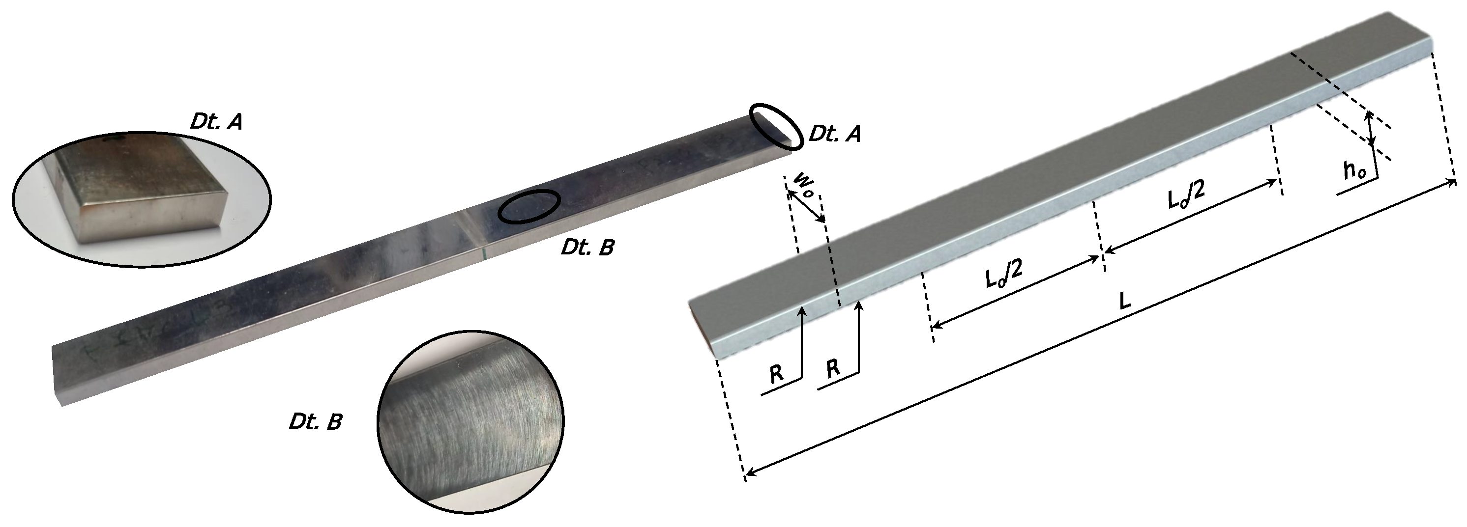
Geometry of the fatigue specimen for three-point in-plane bending testing: left: sample of the actual specimen showing the details of the round corners (Dt. A) and the finishing after milling (Dt. B); right: rendered image of the CAD model showing the dimensions for definition of the specimen geometry.
Metals 15 00315 g004
Figure 5. Representation of the alternating axial tensile fatigue testing machine, its structure, and testing specimen.
Metals 15 00315 g005
Figure 6. Geometry of the smooth fatigue specimen for axial tension: left: sample showing details (Dt. A) of the finishing in the analysis zone: Dt. A—machined; right: rendered image of the CAD model showing the dimensions for definition of the specimen geometry.
Metals 15 00315 g006
Figure 7. 
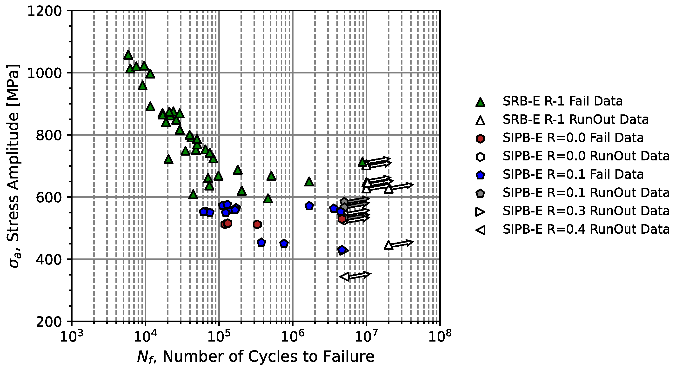
Data pool of fatigue failures and run-outs for specimens tested under rotating and three-point in-plane bending fatigue loadings at different stress ratios. (R—stress ratio, SRB—specimen under rotating bending; SIPB—specimen under in-plane bending; E—elastic regime).
Metals 15 00315 g007
Figure 8. Data pool of fatigue failures and run-outs for specimens tested under uniaxial tension/compression fatigue loadings at different stress ratios. (R—stress ratio, SAT—specimen under subsonic axial tension; UAT—specimen under ultrasonic axial tension; E—elastic regime; EP—elasto-plastic regime).
Metals 15 00315 g008
Figure 9. Walker regression and percentile curves of the normal distribution model considering different stress ratios under bending loading. (R—stress ratio; P f —probability of failure; SRB—specimen under rotating bending; SIPB—specimen under three-point in-plane bending; E—elastic regime; Avg.—average; Dist.—distribution).
Metals 15 00315 g009
Figure 10. Walker regression and percentile curves of the normal distribution model considering different stress ratios with axial tension/compression loading. (R—stress ratio; P f —probability of failure; SAT—specimen under subsonic axial tension/compression; UAT—specimen under ultrasonic axial tension/compression; E—elastic conditions; EP—elasto-plastic conditions); Avg.—average; Dist.—distribution.
Metals 15 00315 g010
Figure 11. PSN field using the ACFC fatigue model considering the mean stress effect due to bending loading conditions. (R—stress ratio; P f —probability of failure; Est.—estimation for run-out data; RB—specimens under rotating bending (elastic conditions); IPB—specimens under three-point in-plane bending (elastic conditions); Avg.—average; Dist.—distribution, 3p—3 parameters).
Metals 15 00315 g011
Figure 12. Probabilistic field using the hyperbolic fatigue model considering the mean stress effect due to tensile conditions from low-cycle regime to very high-cycle regime. (R—stress ratio; P f —probability of failure; Est.—estimation for run-out data; AT (150 Hz)—specimens under axial tension/compression at 150 Hz (elastic conditions); AT (20 kHz)—specimens under axial tension/compression at 20 kHz (elastic conditions); AT (LCF)—specimens under axial tension (elasto-plastic conditions); AT (HCF)—specimens under axial tension (elastic conditions); Avg.—average; Dist.—distribution, 3p—3 parameters).
Metals 15 00315 g012
Figure 13. Probabilistic field using the extended ACFC fatigue model for tension/compression loading conditions, considering the mean stress effect and the generalized plastic regime: (A)—full-field and (B)—zoom in the ψ ε , w axis. (R—stress ratio; P f —probability of failure; Est.—estimation for run-out data; AT (150 Hz)—specimens under axial tension/compression at 150 Hz (elastic conditions); AT (20 kHz)—specimens under axial tension/compression at 20 kHz (elastic conditions); AT (LCF)—specimens under axial tension (elasto-plastic conditions); AT (HCF)—specimens under axial tension (elastic conditions); Avg.—average; Dist.—distribution, 3p—3 parameters).
Metals 15 00315 g013
Figure 14. Walker regression and percentile curves of the normal distribution model considering different stress ratios with axial tensile/compression, axial tensile, and bending loading. (R—stress ratio; P f —probability of failure; SRB—specimen under subsonic rotating bending; SIPB—specimen under subsonic in-plane bending (elastic conditions); SAT—specimen under subsonic axial tension (elastic conditions); UAT—specimen under ultrasonic axial tension (elastic conditions); SATL—specimen under subsonic axial tension (elasto-plastic conditions); Avg.—average; Dist.—distribution.
Metals 15 00315 g014
Figure 15. Probabilistic field using the extended hyperbolic fatigue model for bending and tensile loading conditions, considering the mean stress effect and the generalized plastic regime: (A)—full-field and (B)—zoom in the vertical axis. (R—stress ratio; P f —probability of failure; Est.—estimation for run-out data; AT (150 Hz)—specimens under axial tension at 150 Hz (elastic conditions); AT (20 kHz)—specimens under axial tension at 20 kHz (elastic conditions); AT (LCF)—specimens under axial tension (elasto-plastic conditions); AT (HCF)—specimens under axial tension (elastic conditions); RB—specimens under rotating bending at 25 Hz (elastic conditions); IPB—specimens under three-point in-plane bending at 23 Hz (elastic conditions); Avg.—average; Dist.—distribution; 3p—3 parameters).
Metals 15 00315 g015
Figure 16. Representation of the fracture surface of the rectangular section specimens tested under three-point in-plane bending conditions for a σ a = 515 MPa, σ m = 498 MPa, and R σ = 0.017 0.0 .
Metals 15 00315 g016
Figure 17. Fracture surfaces obtained for different combinations of stress amplitudes and mean stresses under uniaxial loading conditions: (A) σ a = 580 MPa σ m = 710 MPa, (B) σ a = 565 MPa σ m = 690 MPa, (C) σ a = 475 MPa σ m = 580 MPa, (D) σ a = 440 MPa σ m = 540 MPa, (E) σ a = 420 MPa σ m = 515 MPa, and (F) σ a = 420 MPa σ m = 780 MPa.
Metals 15 00315 g017
Figure 18. Magnification of the fracture surface obtained for case Figure 17C ( σ a = 475 MPa, σ m = 580 MPa): left—identification of the initiation zone; right—crack initiation zone from a non-metallic inclusion and formation of a FGA zone.
Metals 15 00315 g018
Table 1. Standard chemical composition of 51CrV4 steel grade in % wt [35].
MaterialCFeSiMnCrVSPb
51CrV4 (EN 1.815)0.47–0.5596.45–97.38≤0.400.70–1.100.90–1.20≤0.10–0.25≤0.025≤0.025
Table 2. Monotonic mechanical properties of the chromium–vanadium alloyed steel, 51CrV4, obtained from ISO 6892-1 standard [35,58].
E [GPa] σ y [MPa] σ uts [MPa] ε f [%] R A f [%]
Average
Std. Dev.  [35]
200.54 ± 6.02 1271.48 ± 53.32 1438.35 ± 73.84 7.53 ± 0.77 34.69 ± 10.39
DIN 51CrV4 (1.8159)20012001350–1650630
Table 3. Average dimensions of specimens used in three-point in-plane bending fatigue testing according to ISO 7438 standard [60].
h 0 [mm] w 0 [mm] I x   [ mm 4 ] L 0 [mm]L [mm]R [mm] R a [ μ m]
6.51 ± 0.04822.05 ± 0.058506.9715020010.664 ± 0.191
Table 4. Average dimensions of smooth specimens used in tensile fatigue test according to ASTM E466-21 standard [61].
d 0 [mm] A 0 [mm2] L 0 [mm]R [mm]Thread [mm]L [mm] L M [mm] R a [ μ m]
3.98 ± 0.2412.41 ± 0.151075M1292201.075 ± 0.610
Table 5. Summary of the regression models considering the effect of mean stress on bending (rotating bending plus three-point in-plane bending), tension/compression, and tensile fatigue testing data using Walker’s model (Equation (3)). (IPB—three-point in-plane bending bending; AT—axial tension/compression; RB—rotating bending).
Fatigue RegimeHCFLCF + HCF + VHCFLCF + HCF + VHCF
Testing Conditions IPB + RB AT IPB + RB + AT
Strength Coefficient, C b 3623.262543.302282.52
Strength Exponent, n b −0.1419−0.0886−0.0888
Coefficient of Determination, R 2 0.57290.67760.4593
Walker Parameter, γ 0.14300.77580.5807
Mean Square Error, M S E 0.27630.59950.7221
Coefficient of Interception, β 0 25.0938.4437.81
Coefficient of Slope 1, β 1 −7.046−11.28−11.26
Coefficient of Slope 2, β 2 −1.008−8.756−6.537
Average Ind. Var1, log σ a ,2.8342.7722.802
Std.Ind. Var1, log σ a ,0.1020.0100.106
Average Ind. Var2, log 2 / 1 R σ ,0.1150.1930.157
Std.Ind. Var2, log 2 / 1 R σ ,0.1600.1930.182
Average Dep. Var, log N f ,4.9655.4635.235
Std. Dep. Var, log N f ,0.7891.3421.146
Table 6. Summary of the estimators for ACFC fatigue model on specimens under bending and tension conditions, considering the ψ ε , w fatigue parameter (Equation (11)). (IPB—three-point in-plane bending bending; AT—axial tension/compression; RB—rotating bending).
Fatigue RegimeHCFLCF + HCF + VHCFLCF + HCF + VHCFLCF + HCF + VHCF
TestingElasticElasticElasto-PlasticElasto-Plastic
ConditionsIPB + RBATATIPB + RB + AT
Dowling Par., γ w 0.85700.22420.22420.4193
Vert. Asymptote, B0.00 (1 [cycle])0.00 (1 [cycle])0.00 (1 [cycle])0.00 (1 [cycle])
Hor. Asymptote, C−2.47 (0.08 [%])−1.87 (0.15 [%])−1.90 ( 0.15 [%])−2.00 (0.14 [%])
Shape Par., β 1.233.153.071.98
Scale Par., δ 4.277.367.086.26
Location Par., λ 13.496.096.488.22
Avg. Rand. Var. v, μ v 17.4812.6712.8113.77
Std. Rand. Var.v, σ v 10.655.255.088.57
Quantile ( P f = 50 % ) 16.6712.6412.7613.42
Disclaimer/Publisher’s Note: The statements, opinions and data contained in all publications are solely those of the individual author(s) and contributor(s) and not of MDPI and/or the editor(s). MDPI and/or the editor(s) disclaim responsibility for any injury to people or property resulting from any ideas, methods, instructions or products referred to in the content.

