Corrosion Behavior of X65 API 5L Carbon Steel Under Simulated Storage Conditions: Influence of Gas Mixtures, Redox States, and Temperature Assessed Using Electrochemical Methods for up to 100 Hours

Abstract

In the context of the deep geological disposal of high-level and intermediate-level long-lived radioactive waste in France, the Callovian–Oxfordian (Cox) clay formation has been selected as a natural barrier. Thus, understanding the corrosion phenomena between the carbon steel used (API 5L X65) for the waste lining tubes and the Cox pore water, as well as its possible future evolutions, is of great importance. A controlled laboratory experiment was conducted using robust handmade API 5L X65 carbon steel electrodes in synthetic Cox pore water under equilibrium with three distinct gas atmospheres, simulating oxic, anoxic, and sulfide-rich environments at 25 °C and 80 °C, in a batch-type electrochemical cell. The experimental methodology involved linear polarization resistance (LPR) cycles, electrochemical impedance spectroscopy (EIS), and Tafel extrapolation at regular intervals over a period of 70 to 100 h to elucidate corrosion mechanisms and obtain corrosion current densities. At the same time, the fluid’s key geochemical parameters (temperature, pH, and redox potential) were monitored for temporal variation. This study, with results showing high corrosion rates under the three conditions investigated at two temperatures, underscores the importance of controlling the immediate environment of the containment materials to prevent exposure to variable conditions and to ensure that corrosion remains controlled over the long term.

1. Introduction

1.1. General Context

In the future French geological disposal facility called CIGEO, high-level waste (HLW) and intermediate-level long-lived radioactive waste (ILW) waste will be buried 500 m deep in the Callovian–Oxfordian (Cox) argillite [1,2,3]. The Cox formation exhibits excellent confinement and retention properties for radioactive elements due to its compactness and low permeability. It is also composed of mineral clay, organic matter, various oxides, and sulfides [4,5,6,7,8,9,10]. At temperatures between 20 and 25 °C at 500 m depth, the argillaceous formation also contains interstitial water, the composition of which has been studied and can be reconstructed using geochemical models [5]. The exothermic nature of the HLW is expected to raise the temperature of the surrounding rock and interstitial water up to 90 °C.

The materials considered for the HLW storage container and the linings are non-alloyed or low-alloy steels. Thus, the HLW repository metallic liner tube will be made of carbon steel (X65 API 5L or CS-X65 or X65), selected by Andra (the French national radioactive waste management agency) based on CS-X65 behavioral studies and mechanical properties. In the current concept, this steel will be separated from the Callovian –Oxfordian clay formation using a cement-bentonite backfilling material. Prior examination of the steel’s corrosion behavior under various conditions is crucial.

The covering steel will be subjected to very varied environments. Initially, the presence of O₂, due to excavations and tunneling, will be quickly consumed. Then, the environment will become anoxic with a partial pressure of CO₂ of approximately 1 atm. Subsequently, the carbon steel corrosion processes will lead to the production of H₂, which will be used by the sulfate-reducing bacteria. This may lead to the arrival of hydrogen sulfides in the environment.

Various corrosion studies have been conducted by Andra using natural Cox pore water obtained directly from in situ drilling under anoxic conditions. These studies, employing electrochemical techniques and mass loss methods [9,11,12,13,14,15,16,17,18,19], report a relatively low corrosion rate (0.02–0.03 mm/yr) and identify magnetite and siderite as the main corrosion products in the absence of sulfides as well as pyrite and mackinawite in the presence of hydrogen sulfides.

This study is part of the same approach of investigating the corrosion rate and mechanisms of CS-X65 in Cox pore water systems. The reconstituted Cox pore water is placed in equilibrium with gas mixtures (oxygen [O₂], hydrogen sulfide [H₂S], and carbon dioxide [CO₂]) representing different stages of the lining environment. The corrosion process will be investigated at first in an anoxic environment but also will consider extreme conditions (a continuously aerated solution and a solution that has undergone significant bacterial sulfate reduction). Experiments were conducted at 25 °C and 80 °C using electrochemical methods over a short duration of a few (3–4) days.

1.2. Influence of the Main Gas and the Temperature on the Corrosion of Carbon Steel

It is widely known that the presence of dissolved oxygen increases the corrosion rate of steel in aqueous environments, because by dissolving in the aqueous system, it directly provides a strong oxidizing agent necessary for the oxidation reaction of this steel [20]. Indeed, the standard potential of oxygen reduction is much higher than that of proton reduction [21]. The corrosion of steel is therefore under the diffusive control of oxygen at the cathode [22]. The concentration of the dissolved oxygen depends on the temperature and the partial pressure of oxygen in the gas in equilibrium with the solution [23]. At atmospheric pressure, the concentration of oxygen in an aqueous environment decreases with increasing temperature. Nevertheless, from room temperature, corrosion in oxygenated aqueous environments (open and therefore at atmospheric pressure) increases with temperature due to the increase in the diffusivity of dissolved oxygen in water. A maximum of corrosion is located at around 75 °C due to the effect of the decrease in solubility with the temperature finally exceeding the effect of the increase in diffusivity. It is then expected to have higher steel corrosion in oxygenated aqueous environments at 80 °C than at 25 °C [24].

In this oxic environment, the corrosion current is given by the cathodic limit current (Equation (2)), corresponding to the reduction of oxygen according to the equation (Equation (1)):

$${O_2}_{\left(aq\right)}+2H_{2}O+4e^{-}\to 4{OH}^{-}$$

(1)

$$i_{corr}=\left|\left.i_L\right|\right.={\displaystyle \frac{4FD{C}_{O_2}}{\delta }}$$

(2)

where, F is the Faraday coefficient, D is the diffusion coefficient of the aqueous oxygen, $C_{O_2}$ is the molar concentration of oxygen, and 4 refers to the number of electrons transferred in Equation (1).

The corrosion products are generally layers of oxides and hydroxides (FeO(OH)·nH₂O) that can somewhat limit the diffusion of oxygen at the interface. In the presence of excess oxygen, the more protective magnetite is less stable and forms with greater difficulty [25,26,27]. FeOOH and Fe₂O₃ are preferentially formed in presence of excess oxygen and Fe₃O₄ when there is a deficit in oxygen in the medium [28].

In anoxic environments, the corrosion is generally lower compared to the oxic environments. In the absence of oxygen, the corrosion rate is determined by the H⁺ concentration (pH) [29]. However, corrosion can still be significant given the presence in the environment of soluble species such as chlorides, carbonates, and sulfides. The presence of dissolved CO₂ acts directly on the pH of the solution [30,31,32]. Indeed, during the solvation of CO₂, carbonic acid H₂CO₃ is formed, a diacid that can release two protons according to Equations (3)–(5):

$${CO}_2+H_{2}O\leftrightarrow {H_{2}CO}_3$$

(3)

$${H_{2}CO}_3+H_{2}O\leftrightarrow H_3{O}^{+}+HC{O}_3^{-}{pK}_{A1}=6.4at25°Cand6.2at80°C$$

(4)

$${HC{O}_3^{-}+H}_{2}O\leftrightarrow H_3{O}^{+}+C{O}_3^{2-}{pK}_{A2}=10.1at25°Cand10.11at80°C$$

(5)

A decreasing pH therefore promotes the corrosion reaction. On the other hand, the formation of carbonates promotes the development of iron carbonates, which are a protective layer for steels [33]. The steel is then covered with a much more protective layer than the iron oxyhydroxides of oxic conditions: either magnetite, Fe₃O₄ (Equation (6)), or an iron carbonate, siderite FeCO₃ (Equation (7)) or chukanovite Fe(OH)₂CO₃ [34]. The siderite is more stable at higher temperatures and can precipitate (Equation (7)) [35,36].

$${3Fe+4H}_{2}O\to {Fe}_3{O}_4+4H_2$$

(6)

$$Fe+2HC{O_3}^{-}\to FeC{O}_3+H_2+{{CO}_3}^{2-}$$

(7)

The presence of sulfides in aqueous neutral/acidic environments is generally associated with an increase in corrosion in these environments [37,38,39]. This is seen in particular in groundwater [40]. Indeed, the sulfide species present at this pH level (H₂S/HS⁻ according to its Sillen diagram) adsorb on the surface of the steel, weakening the interatomic bonds and reducing the activation energy. HS⁻ ions replace OH⁻, and amorphous iron sulfide (FeS_amorphous) and crystalline iron sulfides (mackinawite and pyrrhotite, both are FeS) form deposits on the carbon steel surface. They accelerate the active dissolution of the steel, leading to a reduction in corrosion potentials and broadening the areas of activity. The adsorption of sulfides on the metal surface increases the passive current density. However, an inhibitive effect of H₂S can appear when the concentration is reduced to 0.04 mM [41]. At those concentrations, a metastable mackinawite can be formed, thus converting it into a more protective iron sulfide such as troilite (FeS) and pyrite (FeS₂) [42]. However, the results coming from the literature on groundwaters show that the corrosion of steels in these sulfur-rich environments strongly depends on the chemical composition of these environments (sulfate and chloride content) [43].

In summary, the different atmospheres alter the chemical equilibrium of the solutions, and with the production of Fe²⁺ during the corrosion process, different corrosion products are expected: rather protective against corrosion in anoxic environments, non-protective in aerated environments, and ambivalent in environments containing sulfides.

As for temperature, it accelerates the overall electrochemical processes. Indeed, an increase in temperature is associated with a decrease in activation energy, as well as an increase in the number of active corrosion sites [44]. However, it can also lead to the formation of corrosion products with protective properties, particularly in anoxic conditions with ferrous ions and carbonates.

2. Materials and Methods

2.1. Cox Pore Water Characteristics and Reconstitution of a Basic Pore Water Before Its Equilibration with Three Different Gas Mixtures

2.1.1. Cox Pore Water (CPW)

The basic investigated medium was well-balanced pore water within the Callovian–Oxfordian clay (Cox) formation at Bure (France). The pore water chemistry, in terms of the dissolved major elements [5,45], is given in

Table 1. Pore water chemistry of the Cox formation with major elements reported in mM. SHE is the standard hydrogen electrode.

Elements or Chemistry	Concentration (mM) or Value	Elements	Concentration (mM)
pH	7.35	K	7.07
Redox potential (mV/SHE)	−180	Ca	14.8
Ionic strength	116.0	Mg	14.1
C(4) or carbonate	1.29	Sr	1.12
S(6) or sulfate	34.0	Si	0.0943
Cl−	30.1	Fe	0.0940
Na	32.0	Al	0.0000086

.

2.1.2. Basic Ionic Reconstitution of CPW (Or IRCPW) and Its Equilibration with Its Natural Gas Mixture

To reconstitute the basic ionic composition of the Cox pore water (IRCPW), mineral salts were used.

Table 2. The nature and mass of mineral salts used for the synthesis of 1 L of IRCPW.

Mineral Salts Names and Formulas	Mass (g) for 1 L of Deionized Water
Sodium bicarbonate, NaHCO3	0.445
Potassium chloride, KCl	0.186
Magnesium chloride hydrate MgCl2, 6H2O	1.830
Ammonium sulfate (NH4+)2, SO42−	0.073
Calcium sulfate CaSO4,2H2O	1.416
Calcium chloride, CaCl2 (anhydrous)	1.887
Sodium chloride, NaCl	14.164

presents the nature and mass of the mineral salts to be weighed to produce 1 L of IRCPW, which becomes CPW after it is balanced, by continuous bubbling, with the natural gas mixture (volume percentage CO₂ 1% and N₂ 99%).

2.1.3. Modus Operandi for the Reconstitution of the Three Representative Corrosive Media for the Present Study

In the present study, three different gas mixtures were used to equilibrate, with continuous bubbling, the basic IRCPW. Previously, to find the more suitable gas mixtures for the continuous bubbling, several modelling runs were needed. The content of minerals (in mM) used for the partial reconstitution of the ionic charge of the prospective IRCPW is reported in Table 1. All the parameters, including pH, potential of electrons or pe = −log[electron activity], temperature, and ionic element and gas contents, were inputted for modeling IRXPW using PhreeqC^® Version 3 hydrogeochemical software (United States Geological Survey, https://www.usgs.gov/software/phreeqc-version-3, URL accessed on 5 December 2021) and the ThermoddemV1.10_15Dec2020.dat thermodynamic database generated by BRGM [46].

The final pH, pe, elements, and contents (in mM) in equilibrium with the three gas mixtures were obtained. The gas mixtures are given in a volume percentage:

A: CO₂ (1%), N₂ (99%)

B: CO₂ (20%), H₂S (0.8%), N₂ (79.8%)

C: O₂ (20%), N₂ (80%)

These gas mixtures were ordered from Air Liquide, AlfagazTM (Paris, France).

Once equilibrated by continuous bubbling with their individual gas mixtures, the produced corrosive media are well-balanced waters with the necessary salts for mimicking the dissolved major elements (ionic activity and salinity) and the corresponding dissolved gases. Thus, the corrosive solutions were named as follows:

A: Modified-RCPW or AM-IRCPW

B: Modified-RCPW or BM-IRCPW

C: Modified-RCPW or CM-IRCPW

Equilibration of gas mixture A with the IRCPW aims to simulate the natural Cox water and imitate its physicochemical conditions (pCO₂ = 10⁻² atm).

Equilibration of gas mixture B with the IRCPW constitutes a variant of the physicochemical conditions that may be encountered during the evolution of storage conditions. The corrosion medium imitates a natural Cox water that has suffered the consequences of a strong sulfate reduction by bacteria, responsible for an increase in the partial pressure of H₂S and CO₂. The latter is linked to a strong degradation of organic matter.

Equilibration of gas mixture C with the IRCPW carried out in oxic conditions constitutes a variant relating to the consequences of exposing the Cox rock to air initially during the digging of the galleries.

The bacterial and the pressure factors have not been included in the study regarding the time scale of each experiment (no more than 3–4 days). Biocorrosion is expected under longer periods than those investigated in the present study at the in vitro laboratory scale. Moreover, previous studies on-site showed that the sulfate- and thiosulfate-reducing bacterial strains constitute an aggravating factor of proper physical and electrochemical phenomena investigated here, which are responsible for corrosion and scaling [47].

These three corrosive solutions will be used to study the electrochemical behavior of API 5L X65 steel at two temperatures, namely, 25 °C and 80 °C.

2.1.4. Modelling of the Three Corrosive Media at Two Temperatures

The three corrosive solutions AM-IRCPW, BM-IRCPW, and CM-IRCPW, at the two temperatures (six cases) were also simulated using PhreeqC^® and the ThermoddemV1.10_15Dec2020.dat thermodynamic database [46]. The reason for these simulations is the opportunity for comparison, after obtaining the results of the evolution/interactions of these waters in the absence of carbon steel corrosion (with iron coming only from IRCPW) and in the presence of carbon steel corrosion. Thus,

Table A1. Some contents and supersaturated phases obtained by modeling of AM-IRCPW under condition A [CO₂ (1%), N₂ (99%)]. The presence of iron is only due to IRCPW (9.40 × 10⁻⁵ M) without considering the contribution of iron by corrosion. The supersaturated phases are noted in bold.

Temp. (°C)	[Fe2+] tot	[Fe3+] tot	[H2S] (M)	[HS−] (M)	[CO2]	[HCO3−]
25	9.400 × 10−5	0	0	0	3.322 × 10−4	1.081 × 10−3
80	9.400 × 10−5	0	0	0	1.251 × 10−4	9.983 × 10−4
Temp. (°C)	Phase Name		SI	log IAP	log K (298 or 353 K, 1 atm)
25	Calcite, CaCO3		−0.62	1.22	1.85
	Siderite, FeCO3		−0.76	−1.03	−0.27
80	Calcite, CaCO3		0.40	1.45	1.05
	Siderite, FeCO3		0.23	−0.91	−1.14

,

Table A2. Some contents and supersaturated phases obtained by modeling of BM-IRCPW under condition B [CO₂ (20%), H₂S (0.8%), N₂ (79.8%)]. The presence of iron is only due to IRCPW (9.40 × 10⁻⁵ M) without considering the contribution of iron by corrosion. The supersaturated phases are noted in bold.

Temp. (°C)	[Fe2+] tot	[Fe3+] tot	[H2S] (M)	[HS−] (M)	[CO2]	[HCO3−]
25	9.400 × 10−5	0	7.825 × 10−4	3.493 × 10−5	6.642 × 10−3	1.291 × 10−3
80	9.400 × 10−5	0	3.089 × 10−4	7.211 × 10−5	2.503 × 10−3	1.010 × 10−3
Temp. (°C)	Phase Name		SI	log IAP	log K (298 or 353 K, 1 atm)
25	FeS(am), FeS		−0.76	−3.7	−2.99
	Mackinawite, FeS		−0.22	−3.75	−3.54
	Greisite, Fe3S4		0.98	−20.91	−21.89
80	FeS(am), FeS		0.12	−3.33	−3.45
	Mackinawite, FeS		0.59	−3.35	−3.92
	Greisite, Fe3S4		1.46	−19.83	−21.29

and

Table A3. Some contents and supersaturated phases obtained by modeling of CM-IRCPW under condition C [O₂ (20%), N₂ (80%)]. The presence of iron is only due to IRCPW (9.40 × 10⁻⁵ M) without considering the contribution of iron by corrosion. The supersaturated phases are noted in bold.

Temp. (°C)	[Fe2+] tot	[Fe3+] tot	[H2S] (M)	[HS−] (M)	[CO2]	[HCO3−]
25	0	9.401 × 10−5	0	0	1.291 × 10−3	1.145 × 10−8
80	0	9.401 × 10−5	0	0	1.290 × 10−3	1.637 × 10−7
Temp. (°C)	Phase Name		SI	log IAP	log K (298 or 353 K, 1atm)
25	Maghemite disord. (Fe2O3)		−7.64	−4.80	2.84
	Hematite (Fe2O3)		4.75	−4.80	−0.04
	Magnetite Fe3O4		−25.15	−14.79	10.36
	Magnetite(am) Fe3O4		−29.38	−14.79	14.59
	Goethite, FeOOH		−2.76	−2.40	0.36
	Lepidocrocite, FeOOH		−4.25	−2.40	1.85
	Calcite, CaCO3		−11.15	−9.30	1.85
	Siderite, FeCO3		−18.94	−19.21	−0.27
80	Maghemite disord. (Fe2O3)		1.48	0.30	−1.19
	Hematite (Fe2O3)		3.87	0.30	−3.58
	Magnetite Fe3O4		−8.83	−4.36	4.47
	Magnetite(am) Fe3O4		−12.40	−4.36	8.04
	Goethite, FeOOH		1.43	0.15	−1.29
	Lepidocrocite, FeOOH		0.23	0.15	−0.08
	Calcite, CaCO3		−8.11	−7.06	1.05
	Siderite, FeCO3		−12.72	−13.86	−1.14

of Appendix A present some contents and supersaturated phases, obtained by modeling, for each of three modelled waters AM-IRCPW, BM-IRCPW, and CM-IRCPW at the two temperatures, namely, 20 and 80 °C.

Table A4. Some contents and supersaturated phases, obtained by modeling of AM-IRCPW with A: CO₂ (1%), N₂ (99%). Presence of iron is due to IRCPW (9.40 × 10⁻⁵ M), and to an iron contribution by corrosion ten times higher (9.4 × 10⁻⁴ M). In bold the supersaturated phases.

Temp.(°C)	[Fe2+] tot	[Fe3+] tot	[H2S] (M)	[HS−] (M)	[CO2]	[HCO3−]
25	9.319 × 10−4	8.077 × 10−6	0	0	3.321 × 10−4	2.512 × 10−3
80	7.691 × 10−4	1.709 × 10−4	0	0	1.251 × 10−4	1.888 × 10−3
Temp.(°C)	Phase Name		SI	log IAP	log K (298 or 353 K, 1 atm)
25	Maghemite disord. (Fe2O3)		11.82	14.66	2.84
	Hematite (Fe2O3)		14.70	14.66	−0.04
	Magnetite Fe3O4		14.80	25.16	10.36
	Magnetite(am) Fe3O4		10.57	25.16	14.59
	Goethite, FeOOH		6.97	7.33	0.36
	Lepidocrocite, FeOOH		5.48	7.33	1.85
	Calcite, CaCO3		0.11	1.95	1.85
	Siderite, FeCO3		0.95	0.68	−0.27
80	Maghemite disord. (Fe2O3)		13.48	12.29	−1.19
	Hematite, Fe2O3		7.43	6.15	−1.29
	Magnetite, Fe3O4		18.57	23.04	4.47
	Magnetite(am), Fe3O4		14.99	23.04	8.04
	Goethite, FeOOH		15.87	12.29	−3.58
	Lepidocrocite, FeOOH		6.23	6.15	−0.08
	Calcite, CaCO3		0.95	2.00	1.05
	Siderite, FeCO3		1.66	0.52	−1.14

,

Table A5. Some contents and supersaturated phases obtained by modeling of BM-IRCPW under condition B [CO₂ (20%), H₂S (0.8%), N₂ (79.8%)]. The presence of iron is due to IRCPW (9.40 × 10⁻⁵ M) and iron contribution by corrosion that is ten times higher (9.4 × 10⁻⁴ M). The supersaturated phases are noted in bold.

Temp.(°C)	[Fe2+] tot	[Fe3+] tot	[H2S] (M)	[HS−] (M)	[CO2]	[HCO3−]
25	9.400 × 10−4	0	7.825 × 10−4	7.387 × 10−5	6.640 × 10−3	2.729 × 10−3
80	9.400 × 10−4	0	3.089 × 10−4	1.668 × 10−4	2.502 × 10−3	2.335 × 10−3
Temp.(°C)	Phase Name		SI	log IAP	log K (298 or 353 K, 1 atm)
25	FeS(am), FeS		0.88	−2.11	−2.99
	Mackinawite, FeS		1.43	−2.11	−3.54
	Greisite, Fe3S4		5.76	−16.13	−21.89
	Calcite, CaCO		−1.13	0.72	1.85
	Siderite, FeCO3		−0.26	−0.53	−0.27
80	FeS(am), FeS		1.85	−1.61	−3.45
	Mackinawite, FeS		2.31	−1.61	−3.92
	Greisite, Fe3S4		6.45	−14.85	−21.29
	Calcite, CaCO3		−0.16	0.88	1.05
	Siderite, FeCO3		0.69	−0.45	−1.14

and

Table A6. Some contents and supersaturated phases obtained by modeling of CM-IRCPW under condition C [O₂ (20%), N₂ (80%)]. Presence of iron is due to IRCPW (9.40 × 10−5 M) and the iron contribution by corrosion that is ten times higher (9.4 × 10−4 M). The supersaturated phases are noted in bold.

Temp.(°C)	[Fe2+] tot	[Fe3+] tot	[H2S] (M)	[HS−] (M)	[CO2]	[HCO3−]
25	0	9.409 × 10−4	0	0	1.291 × 10−3	1.156 × 10−8
80	0	9.401 × 10−4	0	0	1.290 × 10−3	1.738 × 10−7
Temp.(°C)	Phase Name		SI	log IAP	log K (298 or 353 K, 1 atm)
25	Maghemite disord. (Fe2O3)		−5.60	−2.76	2.84
	Hematite (Fe2O3)		2.72	−2.76	−0.04
	Magnetite Fe3O4		−22.09	−11.73	10.36
	Magnetite(am) Fe3O4		−26.32	−11.73	14.59
	Goethite, FeOOH		−1.74	−1.38	0.36
	Lepidocrocite, FeOOH		−3.23	−1.38	1.85
	Calcite, CaCO3		−11.14	−9.30	1.85
	Siderite, FeCO3		−17.92	−18.19	−0.27
80	Maghemite disord. (Fe2O3)		3.63	2.44	−1.19
	Hematite (Fe2O3)		6.02	2.44	−3.58
	Magnetite Fe3O4		−5.61	−1.14	4.47
	Magnetite(am) Fe3O4		−9.18	−1.14	8.04
	Goethite, FeOOH		2.51	1.22	−1.29
	Lepidocrocite, FeOOH		1.30	1.22	−0.08
	Calcite, CaCO3		−8.06	−7.01	1.05
	Siderite, FeCO3		−11.65	−12.78	−1.14

in Appendix A present some evolutions in contents and supersaturated phases after considering the presence of supplementary dissolved iron content (coming from corrosion) 10 times higher than that of IRCPW.

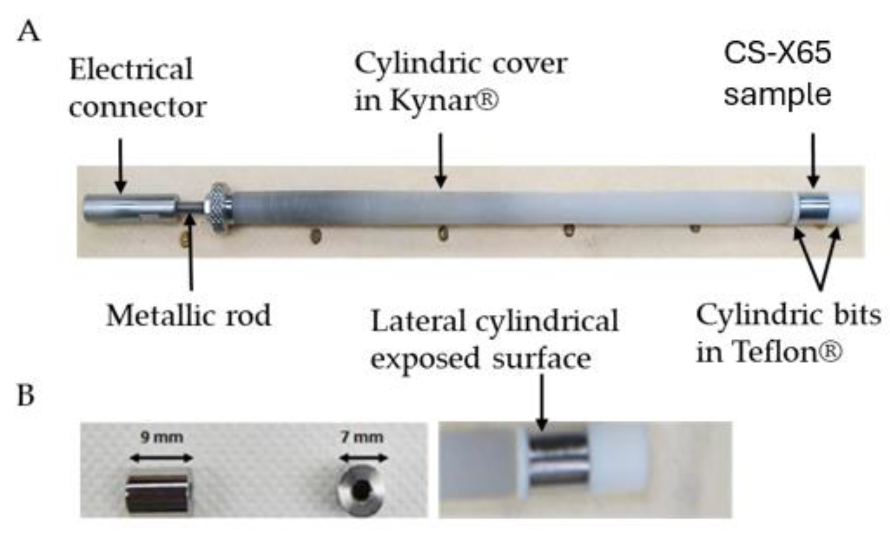
2.2. Carbon Steel API 5L X65 Characteristics and Electrodes Designed for Corrosion Studies

The chemical composition of CS-X65 is given in

Table 3. Carbon steel API 5L X65 chemical composition.

Elements	Chemical Composition (% Mass)
C	0.16
Mn	1.65
Si	0.45
Ti	0.06
P	0.02
S	0.01
V	0.07
Nb	0.05
Fe	~97.53

. The initial source of material is a tubing, which was reprocessed for designing and constructing the API 5L X65 carbon steel electrodes (Figure 1) to be used for the corrosion studies. The homemade 20 cm high CS-X65 working electrode is also presented in Figure 1. It is made of six machined parts. The working CS-X65 electrode is a cylinder of 7 mm in diameter and 9 mm in height with a central threaded hole. The measured roughness of the working electrodes is 0.09 ± 0.001 µm. The lateral exposed surface is 2.00 ± 0.05 cm². The sensitive element is anchored to a CS-X65 made threaded rod whose external electrical contact allows the insertion of a banana plug. The body carrier is a threaded cylinder with a diameter of 9 mm, made of Kynar^® polyvinylidene difluoride (PVDF) from Arkema (Colombes, France), a thermoplastic fluoropolymer with high temperature resistance, low permeability, and high mechanical strength used in applications requiring resistance to acids and hydrocarbons. Two “disposable” PTFE (polytetrafluoroethylene, Teflon^®, from Chemours, Wilmington, DE, USA) cylinders with a diameter of 9 cm are threaded in the center, sandwiching the working CS-X65 surface; a 3 mm thick puck and a 7 mm thick cap, which is three-quarter threaded, are also included. The robust sealing among the working surface, the rod, and the body carrier is ensured by the two PTFE parts and an 8 mm thick threaded steel puck, which sandwich the whole electrode body from the top to the bottom. Steel electrodes are rinsed with ethanol to remove oils, greases, and organic contaminants, and finally rinsed with Milli-Q water, just before immersion in the reconstituted Cox pore water.

2.3. Experimental Setup for Studying the Corrosivity of AM-IRCPW, BM-IRCPW, and CM-IRCPW Waters Against CS-X65

The setup used in this study was designed at BRGM and has also been used for assessing carbon steel corrosion in geothermal environments as well as for inhibition tests. The implementation of this laboratory-scale setup is extensively also described by Betelu et al. [48]. Here, we recall its main characteristics.

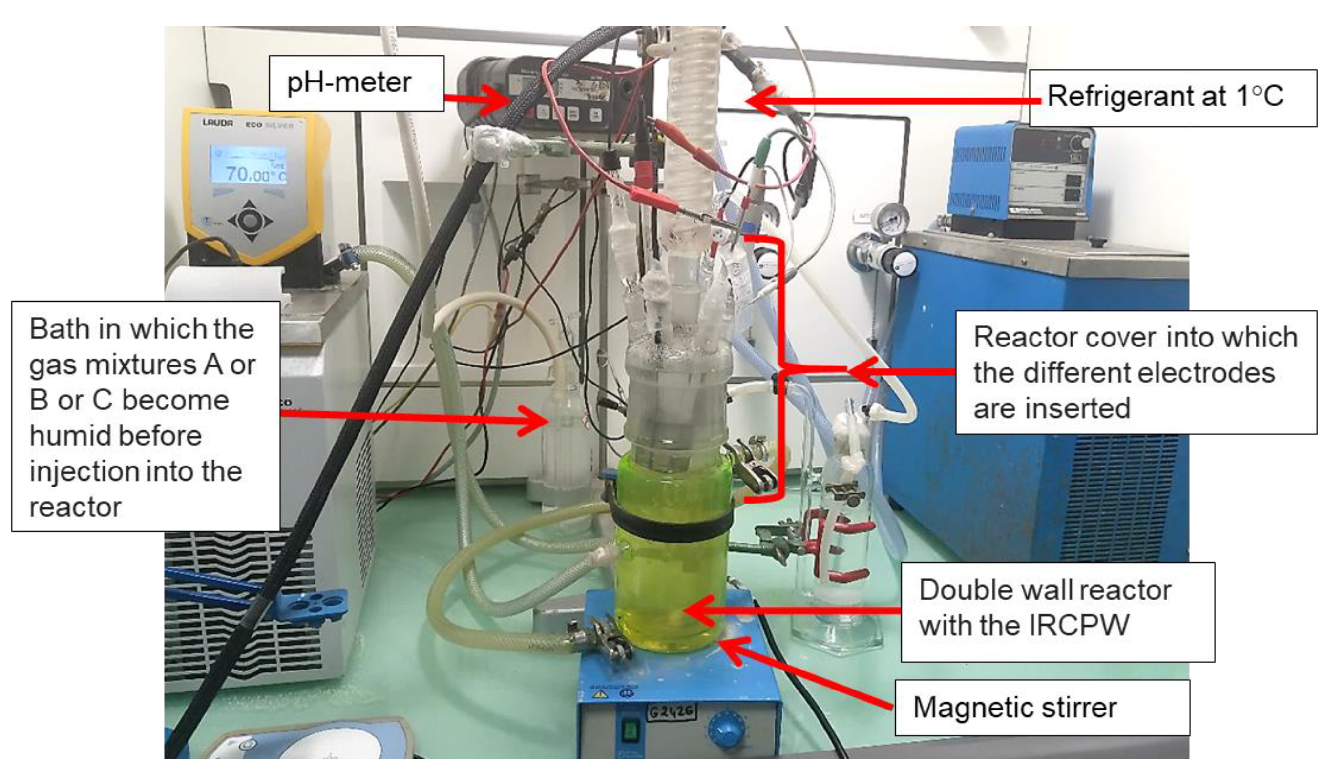
2.3.1. The Electrochemical Reactor

Experiments were conducted in a thermoregulated 1 L cylindrical Pyrex double-walled water-jacketed reactor at 70 °C ± 0.2 °C (Figure 2). A DC10-P5/U thermostat bath (ECO RE 415 S (Lauda Rr.R. Wobser gmbh & Co. KG, Lauda-Königshofen, Germany)) was used to control temperature. The reactor is equipped with a cover with seven conical holes cover into which the following were inserted:

• A refrigerant, into which water flows at 1 °C, was used to condense vapors and minimize losses of AM-IRCPW, BM-IRCPW, and CM-IRCPW waters.
• Six essential electrodes were used to monitor the physical and chemical parameters of the fluid as well as to investigate the reactivity of CS-X65:

  ◦

  A combined pH glass electrode (InLab Reach, Mettler Toledo, Columbus, OH, USA) that was systematically calibrated between each experiment using commercial standard pH buffer solutions (4 and 7);

  ◦

  A platinum wire electrode was used to monitor the Platinum open circuit potential (OCP_Pt or redox potential) versus the internal reference of the pH electrode;

  ◦

  An electrochemical triplet was used only for electrochemical corrosion measurement. It included a CS-X65 working electrode (WE) and a saturated calomel reference electrode (SCE), which consisted of a commercial SCE (K0077 from protected with a KCl 3 mol L⁻¹ junction K0065 both from AMETEK, Inc. Berwyn, PA, USA) and a 6 cm heigh cylindrical Pt/Ir grid counter electrode (CE) with a diameter of 6 cm. The SCE is at approximately +240 mV/SHE;

  ◦

  A CS-X65, called the free electrode, is used to monitor its OCP_X65 without external electrochemical disturbances;

  ◦

  A Pyrex^® tube glass bubbler comprising a dip tube and a diffuser is used for gas equilibration using humidified gas mixtures. The reactor was filled with 1 L of deaerated (humidified N_2, 99.99999%, 1 bar) prospective IRCPW continuously stirred. It was then equilibrated using one of the three humidified gas mixtures before temperature was raised to the desired values at 25 °C or 80 °C.

Figure 2. The 1 L cylindrical Pyrex double-walled water-jacketed reactor is equipped with a cover with seven conical holes into which a refrigerant at 1 °C condenses vapors and minimizes losses of A-, B-, and C-modified IRCPWs. In addition, six electrodes that are used to monitor the physical and chemical parameters of the fluid as well as to investigate the reactivity of CS-X65 were inserted. WEs: 2 CS-X65, RE: SCE, CE: Pt/Ir grid, pH, redox: Pt/SCE. The two thermostatic baths used to control the temperatures of the reactor (from 25 to 80 °C) and the refrigerant (1 °C) as well as the pH meter with temperature compensation are also shown.

Figure 2. The 1 L cylindrical Pyrex double-walled water-jacketed reactor is equipped with a cover with seven conical holes into which a refrigerant at 1 °C condenses vapors and minimizes losses of A-, B-, and C-modified IRCPWs. In addition, six electrodes that are used to monitor the physical and chemical parameters of the fluid as well as to investigate the reactivity of CS-X65 were inserted. WEs: 2 CS-X65, RE: SCE, CE: Pt/Ir grid, pH, redox: Pt/SCE. The two thermostatic baths used to control the temperatures of the reactor (from 25 to 80 °C) and the refrigerant (1 °C) as well as the pH meter with temperature compensation are also shown.

2.3.2. Electrochemical Apparatuses, pH Meter, Data Logger

Electrochemical experiments used a PAR model-2273 potentiostat-galvanostat (AMETEK, Inc., Berwyn, PA, USA) interfaced to a PC system with PAR’s PowerSuite v.2.58 software. A WTW pH Meter (Xylem Analytical Europe, Weilheim, Germany) delivering output signals in volts for temperature and pH was used and connected to a 3700A Data Acquisition System (Keithley Instruments, Inc., Cleveland, OH, USA), handled by a computer using KickStart-1.9.8 software.

2.3.3. Electrochemical Techniques

At the immersion of the CS-X65 WE electrode in the A-, B-, or C-modified IRCPWs, its electrochemical behavior was monitored using various electrochemical techniques.

The corrosion current density (CCD) or J_corr was determined from the electrochemical measurement of the polarization resistance R_p using linear polarization resistance (LPR), Tafel plots (TPs), or electrochemical impedance spectroscopy (EIS). LPR and TPs were measured by polarizing the CS-X65 electrode at ±20 mV and at ±200 mV, respectively, around the OCP_X65 at a scan rate of 0.1 mV·s⁻¹ and 0.166 mV·s⁻¹. Impedance measurements using electrochemical impedance spectrometry (EIS) were performed at the OCP of the CS-X65 over a frequency range of 1 MHz to 1 mHz, using perturbation signals with an amplitude of 10 mV [49]. Knowing R_p, J_corr was calculated using the Stern–Geary equation (Equation (8)) [50,51,52]:

$${\mathrm{J}}_{\mathrm{c}\mathrm{o}\mathrm{r}\mathrm{r}}={\displaystyle \frac{\mathrm{B}}{{\mathrm{R}}_{\mathrm{p}}\times \mathrm{A}}}={\displaystyle \frac{{\mathsf{\beta }}_{\mathrm{a}}{\mathsf{\beta }}_{\mathrm{c}}}{\ln \left(10\right)\times ({\mathsf{\beta }}_{\mathrm{a}}+{\mathsf{\beta }}_{\mathrm{c}})}}\times {\displaystyle \frac{1}{{\mathrm{R}}_{\mathrm{p}}\times \mathrm{A}}}$$

(8)

where J_corr is the corrosion current density (A·m⁻²), B is the Stern–Geary constant (V), R_p is the polarization resistance (Ω·m²), A is the exposed (polarized) surface area of carbon steel (m²), and βa and βc are the anodic and cathodic Tafel constants (V), respectively. The analysis of Nyquist plots of EIS measurements showed an equivalent electrical circuit (EEC), thus revealing and explaining interactions occurring at the carbon steel surface.

All these techniques have been largely investigated and validated in laboratory conditions, more specifically for corrosion so intense that it appears generalized in the presence of high chloride and sulfide levels. At the end of the immersion, the CCD of the electrode was obtained and can be converted, if necessary, into corrosion rates (thicknesses) of mm/y.

2.3.4. Gravimetric or Mass Loss Technique

The gravimetric technique, which is used to estimate the corrosion thickness loss, is based on an experimental determination of weight loss (W_loss) and the exposed surface area (A) of samples of carbon steel profiles after the attack by exposition (immersion) to corrosive SRGW by means of a chemical treatment including an inhibitor in solution to minimize overoxidation of the metal surface once the corrosion products have been fully eliminated. A norm was applied for this work [53] and a detailed procedure can be seen in reference [54]. CS-X65 rough samples were first rinsed with milliQ 18 MΩ water and ethanol, dried with compressed dinitrogen, and weighed (W_bexp (in g) is the weight of sample before immersion). After CS-X65 interaction with the SRGW, cylinders underwent desquamation. Corrosion products were removed by immersing the cylinders in Clarke’s solution (20 g antimony trioxide (Sb₂O₃), 50 g stannous chloride (SnCl₂), and 1 mL 38% hydrochloric acid (HCl)) for 5 min before rinsing the sample with milliQ 18 MΩ water and ethanol, drying with N₂, and weighing. The operation was repeated five times to draw the linear evolution of the mass versus time. The y-intercept is the representative mass of the sample after exposure to A-, B-, and C-modified IRCPWs (W_aexp (in g) is the weight of sample after exposure). From the gravimetric experiment, the corrosion thickness loss equation (Equation (9)), CR_g, was obtained from the relationship of the weight loss W_Loss (in g) = W_bexp − W_aexp, with the volumetric mass (or density) of the iron ρ (0.00785 g·mm⁻³), exposed surface area of specimen A (in mm²) and immersion time T (in years):

$$CRg\left({\displaystyle \raisebox{1ex}{$\mathrm{m}\mathrm{m}$}\!\left/ \!\raisebox{-1ex}{$\mathrm{y}$}\right.}\right)={\displaystyle \frac{Wloss}{\rho TA}}$$

(9)

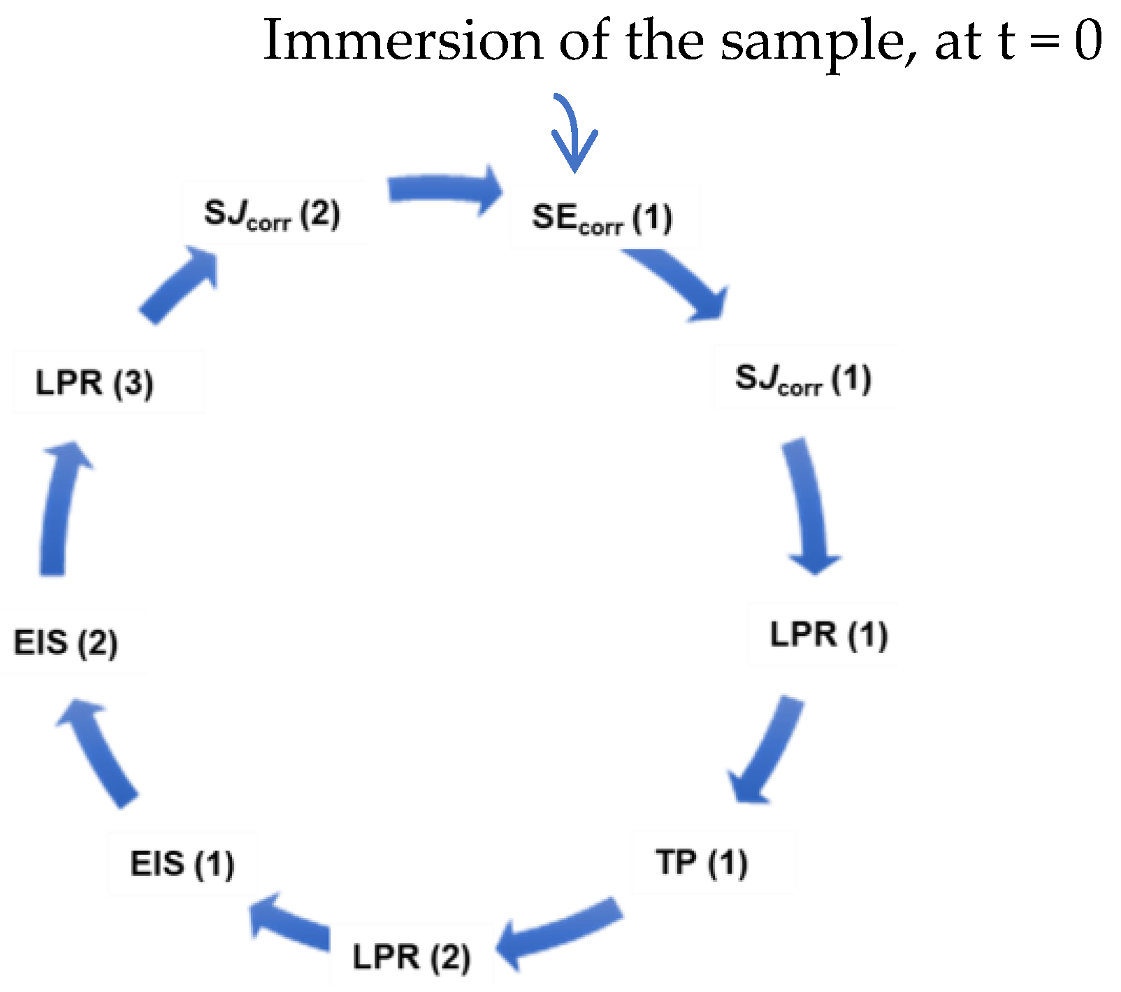
2.3.5. Electrochemical Study

Stationary (LP and TP) and transitory (EIS) electrochemical technics were consecutively applied to the CS-X65 working surface in a loop with precise order and timing (Figure 3) to investigate the mechanisms of the interaction between CS-X65 and A-, B-, and C-modified IRCPWs.

Here,

-

SE_corr: monitoring of the free corrosion potential E_corr;

-

SJ_corr: monitoring of the corrosion-free current J_corr to the corrosion-free potential E_corr;

-

LPR: linear polarization resistance measurement, allowing access to J_corr;

-

TP: linear polarization (drawing of the Tafel curves);

-

EIS: measurement of impedance by EIS at E_corr.

The loop was carried out between a minimum of 18 times and a maximum of 25 times for an immersion duration of 72 to 98 h.

The electrochemical behavior of CS-X65, when immersed in A-, B-, and C-modified IRCPWs, enables their proper measurements and comparison. All the experiments in the six different environments were conducted twice to ensure good reproducibility.

2.4. Scanning Electron Microscopy (SEM) Characterization

For a better understanding of the corrosion processes influenced by the CS-X65 surface deposits, the surface morphology of the CS-X65 electrode was analyzed using scanning electron microscopy (SEM), specifically for Condition B, in the presence of sulfide and carbon dioxide. At the end of the experiment, the CS-X65 electrode was immersed in liquid nitrogen under an inert atmosphere before being placed under the microscope. The CS-X65 surface was then analyzed to examine its morphological characteristics with secondary electrons and backscattered secondary electrons using Tescan Mira 3 equipment coupled to an energy dispersive X-ray (EDX) system (Gaithersburg, MD, USA).

3. Results

3.1. pH and E_Pt Temporal Evolutions Under the Three Conditions at Two Temperatures

3.1.1. pH Temporal Evolutions

For the three conditions named A, B, and C, continuous measurements of the pH and redox potential of the solutions are carried out during the immersion time. Figure 4 shows these temporal evolutions of pH and redox potential (obtained by a Pt/SCE electrode) under the three conditions and at two different temperatures, namely, 25 °C and 80 °C.

In each case, a rapid stabilization of the pH is observed, conditioned by the solubilization of CO₂ and H₂S. Indeed, the nature of the mixture of gases used for bubbling, as well as the temperature influence the pH, the redox potential, the sulfide content, and the alkalinity of the solution, are reported. The content of dissolved CO₂ in the solution acts directly on the pH by lowering it. When CO₂ is solvated, carbonic acid H₂CO₃ is formed. This is a diacid that can release two protons according to Equations (4) and (5) [55].

By bubbling with CO₂ only (condition A), the pH stabilizes in a few minutes, and the solution obtained is slightly more acidic at 25 °C (pH = 6) than at 80 °C (pH = 6.2) (Figure 4A). This is explained by the fact that the solubility of CO₂ in water is higher at low temperatures. This compensates for the usual increase in pH when the temperature decreases.

Under condition B, in addition to CO₂, H₂S also contributes to the acidification of the solution (Figure 4B). As for carbon dioxide, H₂S behaves as a weak diacid in solution, according to Equations (10) and (11) [56]:

$$H_{2}S+H_{2}O\to {HS}^{-}+H_3{O}^{+};{pK}_{A1}=7.00at25°Cand6.53at80°C$$

(10)

$${HS}^{-}+H_{2}O\to S^{2-}+H_3{O}^{+};{pK}_{A2}=12.97at25°Cand11.57at80°C$$

(11)

The pH measurement in the solution with bubbling of mixture B gives a value of 4.5 at 25 °C, which is more acidic than bubbling at 80 °C (4.8–5.2); these values are lower than those obtained under condition A.

In the case of condition C, where O₂ and N₂ are bubbled, the measured pH is neutral (pH = 7.00 at 80 °C) or close to it (pH = 6.00 at 25 °C). The further decrease in pH (Figure 4C) can be related to the greater auto-ionization of water at a higher temperature [24].

3.1.2. E_Pt Temporal Evolutions

Under condition A, the redox potential obtained is almost similar for both temperatures. It varies (Figure 4A) between −300 and −200 mV/SCE KCl 3M (−60 and +40 mV/SHE). The anoxic conditions in the cell are therefore reached, but they are not as anoxic as the measured values of the Cox water on site (−210 to −180 mV/SHE) [57]. In Figure 4A, the fluctuations in the redox potential are caused by the electrochemical measurements carried out nearby, in particular the Tafel method, which imposes overvoltages of several hundreds of mV, disturbing all the other nearby potentiometric measurements.

Under condition B (Figure 4B), at 25 °C, we observe a stabilization of the potential, reaching −250 mV/SCE, like condition A, due to anoxic conditions. A drop in potential is observed around 40 h, which can be linked to the presence of the SO₄²⁻/S²⁻ couple, known to shift the potential toward more cathodic values. Indeed, there might have been a delay in the platinum electrode’s sensitivity to the sulfides entering the solution. At 80 °C, larger fluctuations due to the polarization of the steel are present, making data analysis more challenging. The redox potential typically varies between −360 and −240 mV/SCE (−138 to −18 mV/SHE).

Under condition C (Figure 4C), the pH equilibrium when bubbling air continuously is close to 6 at 25 °C and between 6.0 and 7.4 at 80 °C. The redox potential is higher than that noted under conditions A and B due to the presence of oxygen. Here, we have 150–230 mV/SCE (372–452 mV/SHE) at 80 °C and 120–130 mV/SCE (360–370 mV/SHE) at 25 °C. These are typically the values found in aerated and stirred solutions [58]. The main redox couple that determines the potential is therefore O₂/H₂O. Similarly, the higher redox potential at 80 °C can be explained by the increase in the standard potential of the O₂/H₂O coupled with temperature, as demonstrated by the Nernst equation.

3.2. E_X65 Temporal Evolutions Under the Three Conditions at Two Temperatures

The temporal variations of the E_X65 (or OCP_X65) under the three different controlled atmospheres are given at 25 °C and 80 °C in Figure 5. Initially, higher OCP_X65 values are observed under air bubbling condition C. The presence of oxygen, and therefore the O₂/H₂O redox couple, shift the OCP_X65 toward more anodic values [58]. Furthermore, as with the redox potential, the OCP_X65 (which is a mixed potential) is higher at 80 °C due to the effects of temperature on the thermodynamics of the O₂/H₂O couple. In this case, a higher OCP_X65 does not mean an ennoblement of the steel compared to the other conditions.

For atmospheres A and B, there is a temporal stability of the OCP_X65 values, which are mainly impacted by the temperature. Indeed, the most cathodic OCP_X65 values are obtained at 80 °C, and the values are very close for these two atmospheres A and B (around −820 mV/SCE (−640 mV/SHE)). Since sulfides generally drive the OCP_X65 toward very negative values, it is interesting to note here that the OCP_X65 value is lower at 80 °C, while H₂S is more soluble in water at 25 °C [56].

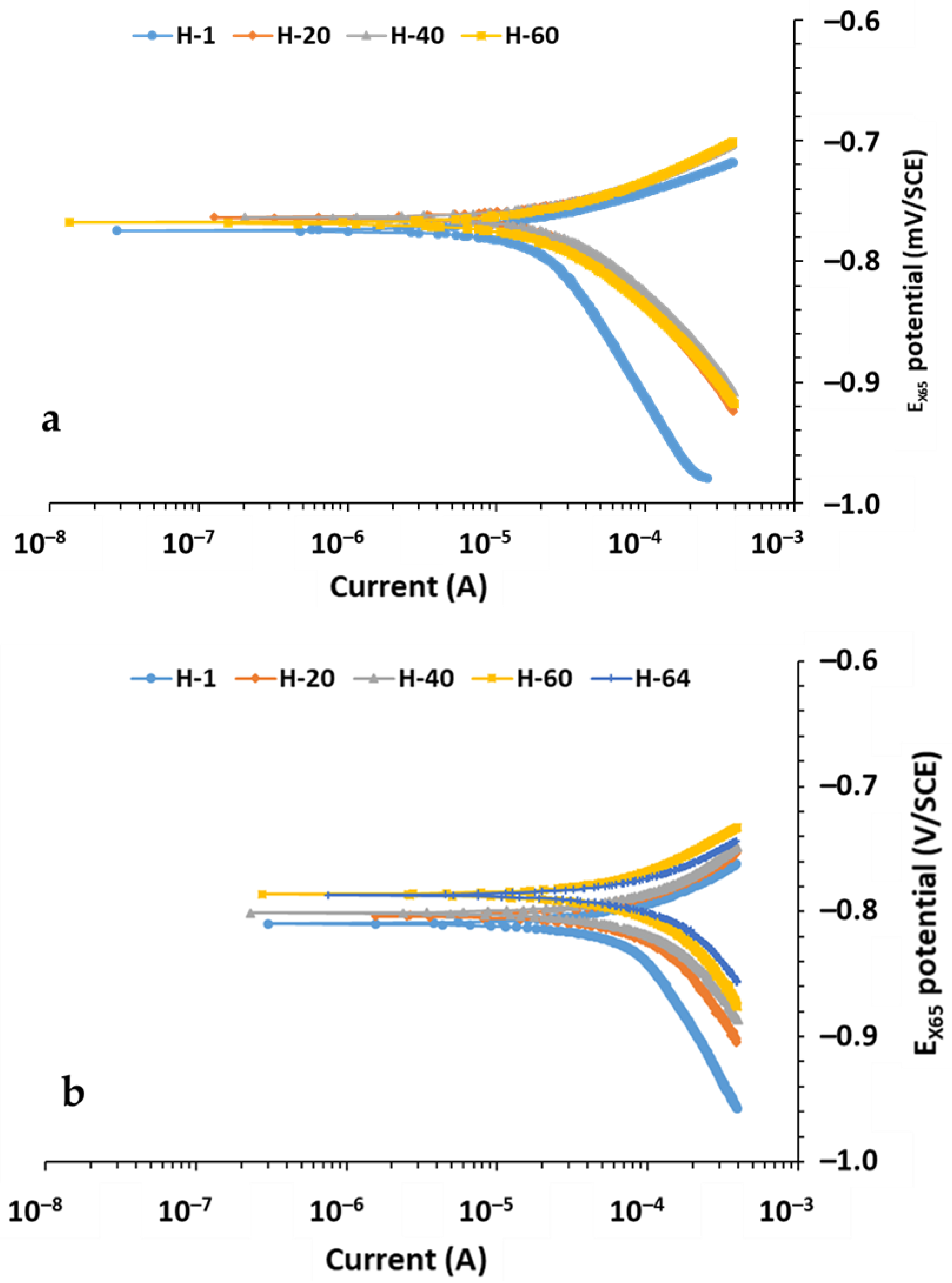
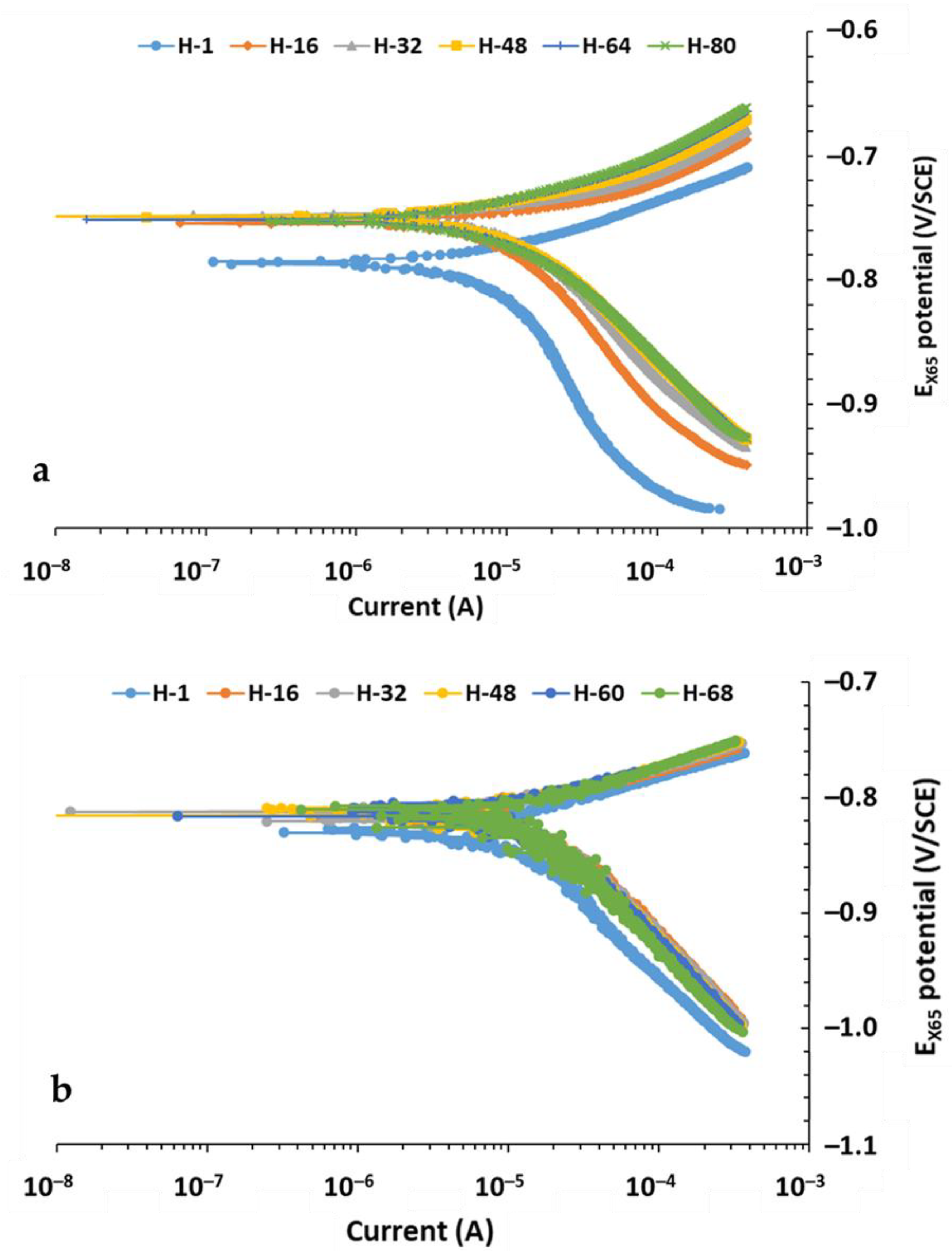
3.3. Tafel Results Under the Three Conditions at Two Temperatures

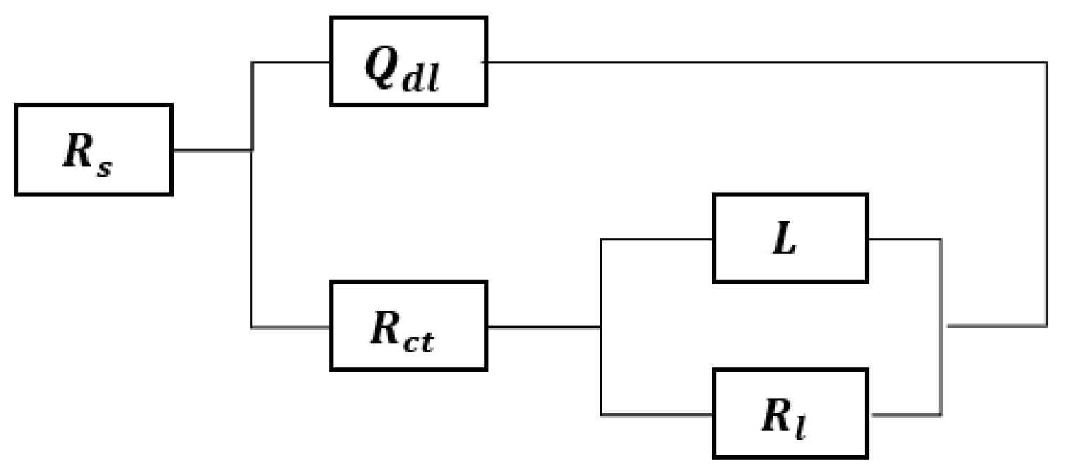
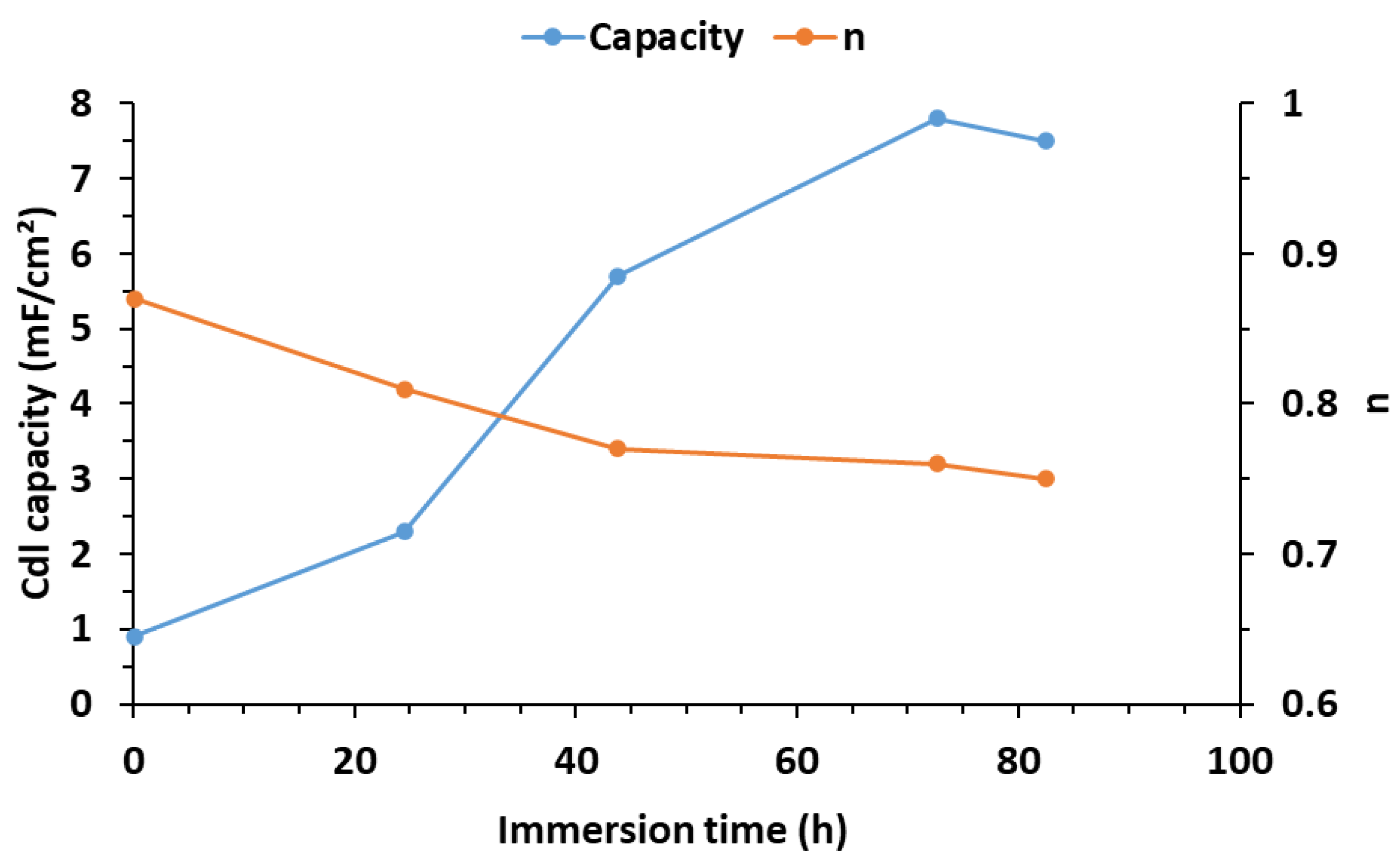
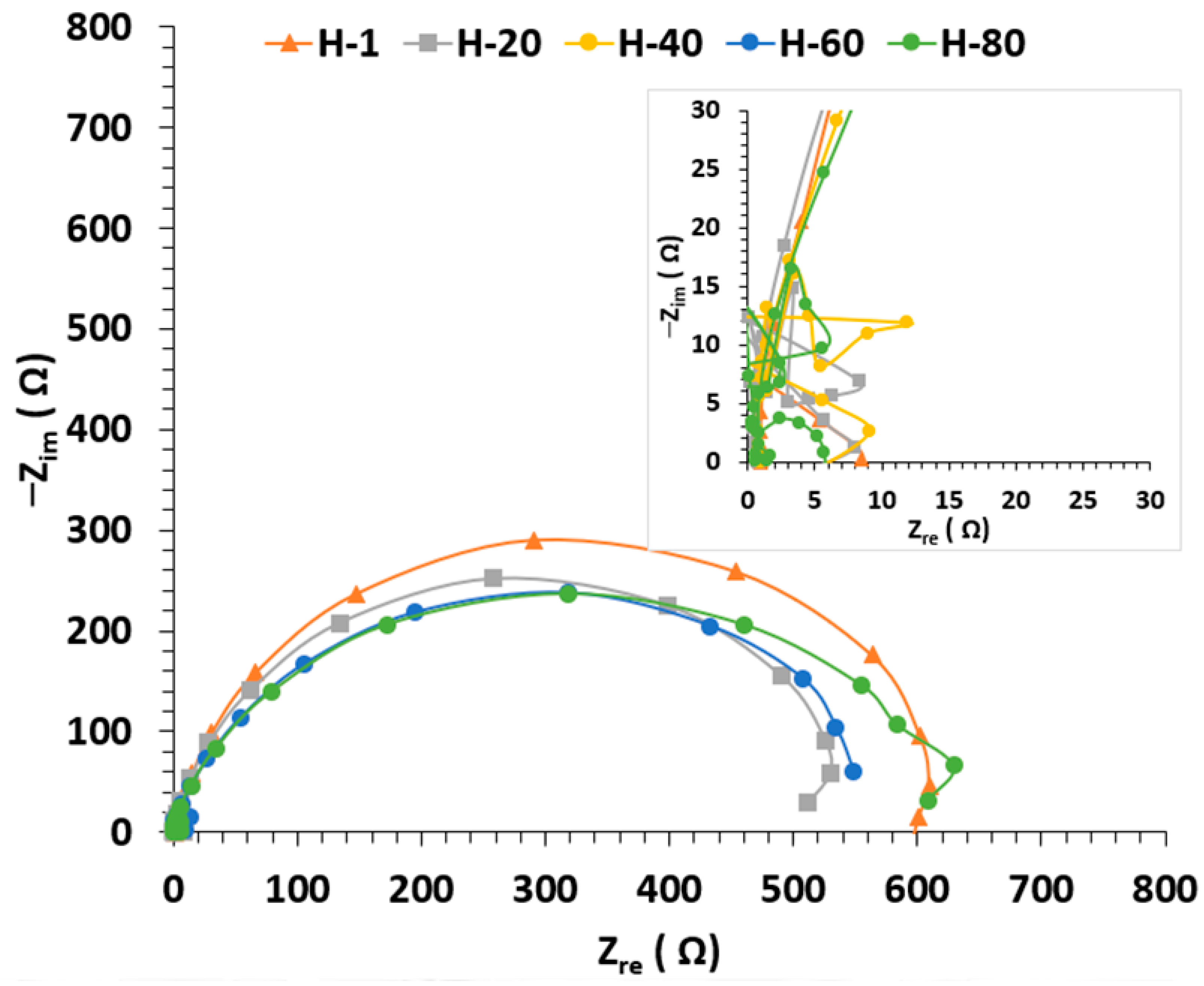
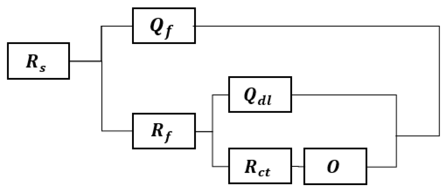
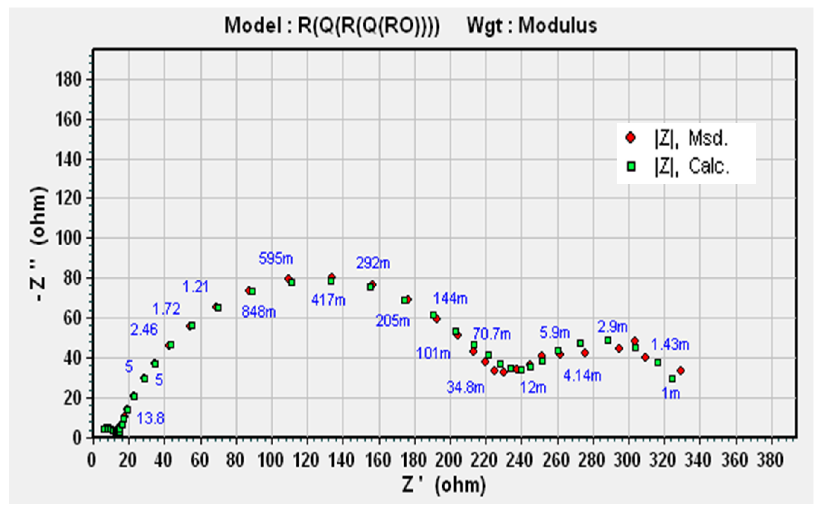
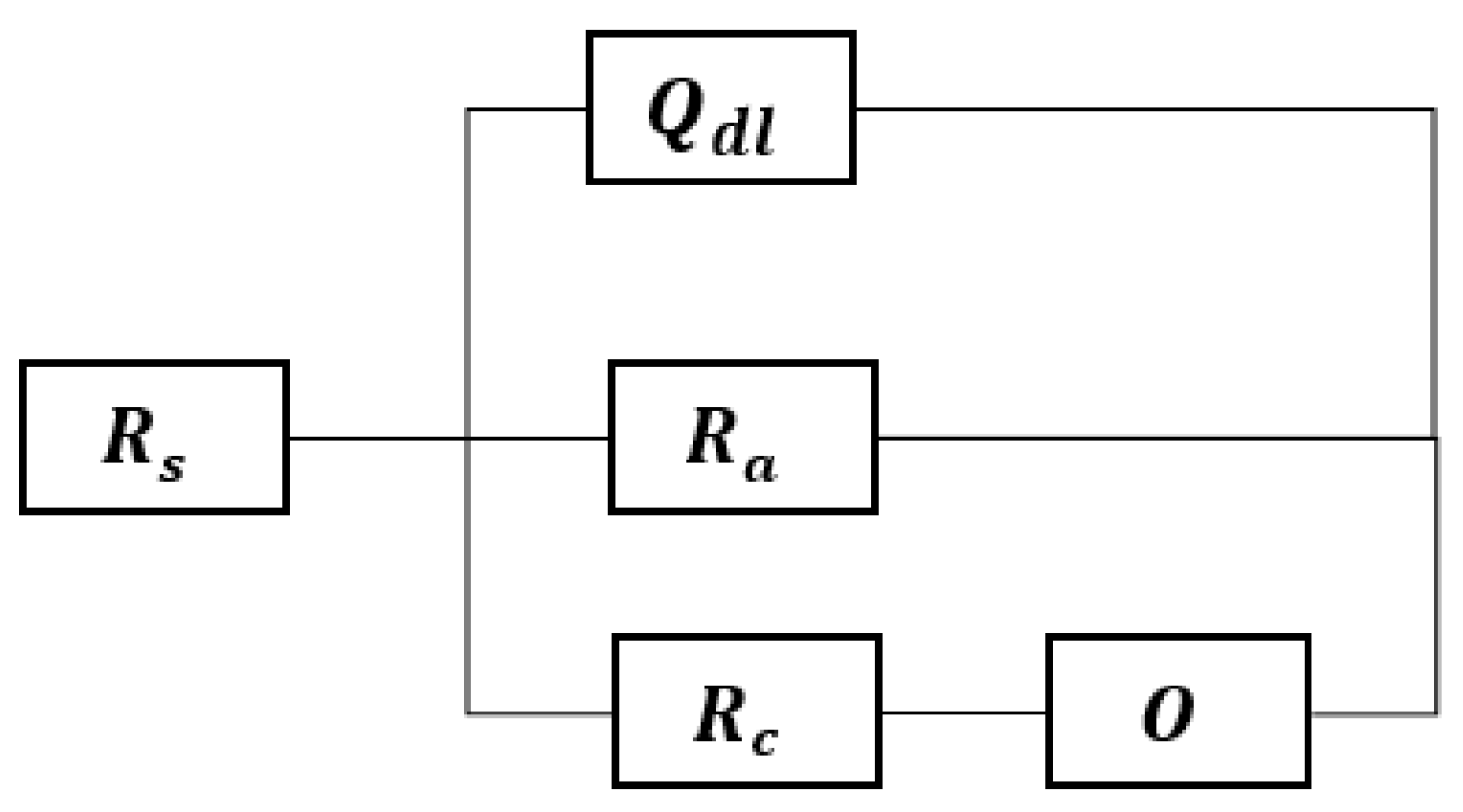
The plot of polarization curves allows, through the Butler–Volmer equations, the determination of the kinetic parameters associated with corrosion, by applying the Tafel method. A corrosion potential (E_corr), a corrosion current density, and anodic and cathodic transfer coefficients are then determined. However, in the presence of diffusion processes, the validity of the kinetic parameters related to corrosion obtained is debatable.

Figure 6a,b show the evolution of the I-E characteristic curves obtained over time (from the first hour of measurement, H-1, to H-80) with the CS-X65 under condition A (99% N₂ and 1% CO₂) at 25 °C and 80 °C, respectively. The E_corr values obtained from the Tafel curves (Figure 6, Figure A1 and Figure A2 in the Appendix A) are almost similar to those obtained from the OCP_X65 measurements (Figure 5) under the same bubbling conditions before the ±200 mV polarizations (a difference of approximately 3 to 23 mV between OCP_X65 and E_corr have been found). This indicates a limited effect of the capacitive current during the polarization of the steel [59].

At 25 °C, there is a quasi-stability of the strong anodic activity (βa between 40 and 60 mV/decade). However, there is an increase in the cathodic activity, which is reflected by the fall in the value of the Tafel cathodic slope over time (βc = 180 mV/decade at the beginning of the experiment followed by stabilization around 110 mV/decade after a few hours). The corrosion is therefore under cathodic control. Thus, after 48 h, at 25 °C, βc = 112 mV/decade, while βa = 48 mV/decade. This, therefore, results in a Stern–Geary coefficient of B = 14.5 mV and a corrosion current density (CCD) of 9.87 µA cm⁻². At 80 °C, the curves show less variability over time. After 48 h, the values acquired for βa (53 mV/decade), βc (107 mV/decade), and B (14.4 mV) results in a CCD of 5.35 µA cm⁻².

The polarization curves versus time, under B and C conditions, are given in Appendix A, Figure A1a,b and Figure A2a,b). The temporal evolutions of the Tafel curves at 25 °C and 80 °C permit the analysis of the evolution over time of the kinetic parameters associated with oxidation and reduction phenomena on CS-X65.

Figure 7 shows the stabilized I-E curves using all operating conditions after 48 h (physicochemical equilibrium). The E_corr values obtained from the Tafel curves are like those obtained from the OCP_X65 measurements prior to each polarization. This indicates a limited influence of capacitive or inductive currents during the potentiodynamic measurements, at least around E_corr [60,61].

For condition B, in the presence of sulfides, the Tafel curves quickly exhibit a linear behavior allowing the use of the Tafel adjustment. Initially at 25 °C, the anodic βa and cathodic βc coefficients are 43 and 202 mV/decade, respectively, which corresponds to B = 15.5 mV. The cathodic activity then increases to βc = 111 mV/decade after 80 h and βa = 80 mV/decade for B = 20.3 mV. The measured CCD increases from 20 to 42 µA cm⁻² after 80 h. The increase in the CCD could be linked to a greater role of the sulfides in the corrosion process. Indeed, a decrease in the redox potential was observed in this condition after 40 h, suggesting an increase in sulfides. However, we observe an increase in the βa, which implies a decrease in anodic activity, suggesting a slowdown in the oxidation process, probably due to the formation of a pseudo-passive layer. The overall current is still higher due to the increase in cathodic activity.

At 80 °C, the anodic activity is constant (βa = 60–70 mV/decade) throughout the experiment), and the βc goes from 270 to 115 mV/decade. B then varies between 20 and 30 mV. The CCD remains generally constant, between 95 and 100 µA cm⁻².

The Tafel curves of condition C (Appendix A, Figure A2a,b) under conditions of air bubbling show a clear decline in CCD at cathodic potentials at 25 °C. Indeed, when the model is adjusted by considering pure activation kinetics, very high Tafel cathodic slope values are obtained, to the point of becoming almost infinite (vertical cathodic part). This decline in cathodic activity is obviously attributed to the diffusion of oxygen due to the limited solubility of O₂ in water. Diffusion limitation is observed despite the agitation of the solution. The shape of the curves obtained suggests mixed activation–diffusion kinetics [62]. A limiting current for oxygen reduction can then be found: 356 µA cm⁻² at the start of the experiment and 136 µA cm⁻² after 16 h of immersion. The CCD is obtained by fitting only the anodic part of the curve. Under the pure activation regime, we obtain values of 122 and 41 µA cm⁻², respectively. The CCD decreases regularly from 41 to 28 µA cm⁻² (B varies between 24 and 30 mV) and stabilizes until the end of the experiment. At 80 °C, the diffusive component does not disappear due to a lower solubility of oxygen. Indeed, the CCDs obtained are much higher (200–600 µA cm⁻²), and the kinetics of iron oxidation are accelerated by the temperature. The curves with air bubbling also present a rapid increase in current density at very high cathodic over-voltages, which is attributed to a new electrochemical reaction (probably the reduction of water).

In summary, the linear polarization measurements for the Tafel method have provided insight into the mechanisms involved in corrosion, particularly diffusion in the cathodic process in the presence of oxygen, as observed by the very high values of the cathodic transfer coefficients. The EIS measurements, presented below, will provide more information on these mechanisms.

3.4. EIS Results

3.4.1. Condition A (CO₂ 1%, N₂ 99%)

Figure 8 shows the evolution of the Nyquist mode diagrams at 25 °C under condition A. The diagram is presented in the form of a main loop attributable to the charge transfer (and therefore to the corrosion process). The variations obtained at very high frequencies (HFs) (>10 KHz) are difficult to interpret and are probably a measurement artifact or due to the presence of ferric ions randomly dispersed on the surface, conferring no protective character. An additional phenomenon in the form of an inductive loop, observed in Figure 8 after 1 h and 1 day of immersion, appears at low frequencies. This phenomenon is attributable to the adsorption –desorption of electroactive species such as H⁺ protons or Cl⁻ ions [63]. The intensity of the inductive loop decreases until it disappears completely at the end of the experiments. The influence of these adsorbed species could intervene in the potentiodynamic curves, in the form of an induction current, at anodic overvoltages. The size of the inductive loop decreases with time until it is no longer directly visible on the Nyquist diagram after 48 h.

An EEC, R(Q(R(LR)), corresponding to the first 30 h, allowing induction to be taken into account, is presented in Figure 9 [64]. It comprises an electrolyte resistance (R_s) in series with a CPE (Q_dl) in parallel with a charge transfer resistance (R_ct) as well as an induction (L) in parallel with a resistance (R_l).

By obscuring the points obtained at very HFs (>10 kHz), the comparison of the simulated data with the experimental data shows a good fit. Omitting some very high or very low frequency data points does not interfere with the model validation [65]. The simulated values of electrical elements are given in

Table 4. Results of the simulation of the impedance obtained at two immersion times (after 24 and 96 h) under condition A at 25 °C; A = 2 cm².

Circuit Element	Immersion Time
	24 h		96 h
	Value	Relative Error (%)	Value	Relative Error (%)
Rs (ohm)	10.5	0.9	5.3	1.1
Q-Yo	6.407 $\times$ 10−3	1.4	2.042 $\times$ 10−2	1.4
n	0.81	0.7	0.774	0.8
Rct (ohm)	636	2.6	459	2.5
L(H)	1.029 × 104	17.1	-	-
Rl (ohm)	258	10.8	-	-
Cdl calculated (F)	4.35 $\times$ 10−3	-	6.9 $\times$ 10−3	-

. Parameters such as R_tc and the double layer capacitance are then determined (Figure 10).

At 24 h, the constant phase element (CPE or Q_dl) attributed to the double layer is characterized by a coefficient of dispersion of n = 0.81, which reflects a distribution of capacities on the surface of the steel. The associated cut-off frequency $f_c$ is 20 mHz. The relation Equation (12) allows its capacity to be calculated:

$$Cdl=Y_0{\left({\omega }_c\right)}^{n-1}=Y_0{\left(2\pi f_c\right)}^{n-1}$$

(12)

where $Cdl$ is the double layer capacitance, Yo the admittance of the CPE, and ${\omega }_c$ is the cut-off angular frequency.

The obtained double layer capacitance is 2.18 mF cm⁻², which is much higher than what is usually observed with the double layer values of carbon steels (about 100 µF cm⁻²) [66]. This high value may be due to the relaxation of another adsorbed intermediate species, with a higher time constant, and would interfere with the double layer. By introducing into the proposed circuit, a component linked to this relaxation, the capacitance values always remain high. Another explanation would be an interference due to the layer of corrosion products. If it is powdery and conductive, it would lead to an increase in the specific surface area of the steel compared to the primary current distribution. The effective polarizable surface would then be much larger and could explain the high capacitance values observed (capacitance is an indirect measurement of the interface surface area), as well as part of the observed capacitance distribution. In the experiment carried out (Figure 11), the calculated capacity increases with time while the value of the coefficient n decreases simultaneously, reinforcing this second hypothesis [67,68,69].

Beyond 30 h, the inductive component disappears, and the R(QR) circuit (simplified Randles) correctly simulates the data. Table 4 gives the simulation results after 24 and 96 h with the two proposed circuits.

A decrease in the charge transfer resistance is observed, showing the non-protective nature of this layer of corrosion products until stability is attained after 48 h and during the following 48 h. As shown in Figure 12, at 80 °C, only one capacitive loop is visible in the Nyquist diagram, varying very moderately during the experiment. The points at very high HFs are also considered as measurement artifacts.

The inductive contribution is also suspected in the case at 80 °C. Indeed, at H-1, the end of the curve at low frequencies shows the beginning of a curvature of the curve toward the inside. It would certainly have been more visible if the experiment had been conducted on lower frequencies such as 1 mHz. This inductance is however not sufficiently influential to weigh down the EEC at low frequencies. On the other hand, the analysis of the phase variation in the Bode diagram reveals the existence of an additional time constant between 1 Hz and 1 mHz, which we tried to model using the circuit R(Q(R(QR)) [64,70] (Figure 13), i.e., an additional pseudo-capacitance associated with adsorption and desorption phenomena on the surface of the steel. It gives satisfactory results (

Table 5. Results of the impedance simulation obtained under condition A at 80 °C after 1 h of immersion time; A = 2 cm².

Circuit Element	Value	Error (%)
Rs (ohm)	9.3	0.96
Q-Yo	2.701 × 10−3	4
n	0.99	0.9
Rct (ohm)	150.1	21
Q-Yoi	1.834 × 10−3	9.5
ni	0.94	5.2
Ri (ohm)	459.6	7.4

).

At 80 °C, if we consider a single CPE, the distribution of capacities are less important (n > 0.94 during the whole experiment) than previously noted. With the proposed circuit, we find (n > 0.97) for the CPE of the double layer, which can be assimilated to a pure capacitance. The values of the capacitance obtained always remain high (1.35 mF cm⁻²). The simulation shows that a large part of the polarization resistance is in fact due to the pseudo-capacitive phenomenon obtained at low frequencies. Linear polarizations are therefore not suitable for the evaluation of the corrosion rate in these cases. No passive film in HF is identified on the two curves in the Nyquist diagram, suggesting that the steel remains in an active state during the whole experiment.

3.4.2. Condition B (H₂S 0.8%, CO₂ 20%, N₂ 79.2%)

The temporal evolution of the impedances obtained under condition B is presented in Figure 14. At 25 °C, as with the bubbling of mixture A, a start of adsorption in the low frequencies at the very beginning of the immersion is revealed. The sulfides are easily adsorbed on the Fe(SH)–ads interface in acidic environments (pH = 4 here) [71]. The iron oxidation reaction can then be described using Equations (13)–(15):

$$Fe+H_{2}O+H_{2}S\to Fe{\left({HS}^{-}\right)}_{ad}+{H_{3}O}^{+}$$

(13)

$$Fe{\left({HS}^{-}\right)}_{ads}\to Fe({HS)}^{+}+{2e}^{-}$$

(14)

$$Fe({HS)}^{+}+{H_{3}O}^{+}\to {Fe}^{2+}+H_{2}O+H_{2}S$$

(15)

The proposed EEC, R(Q(R(LR))), of Figure 15 provides a good superposition with the experiment. The different parameters thus obtained present errors of the values lower than 10%, and errors lower than 20% are obtained for the parameters associated with the inductance. The use of frequencies lower than the mHz would have been necessary to reduce the error on the measurement. From 24 h, a classic R(QR) circuit adjusts the data well, and the induction phenomena are eclipsed by the capacitance of the interface, which increases.

At 80 °C, the same EEC considering adsorption at low frequencies is used at the beginning of the experiments. However, after 20 h of immersion, at low frequencies, a new time constant is highlighted. The loop no longer has its characteristic rounding at low frequencies. The introduction of a component linked to diffusion makes it possible to model the data. The Randles EEC R(Q(RW)) is then used. The diffusional process is linked to the reduction of hydrogen sulfide at the electrode (Equation (16)), which directly contributes to the reverse reaction of iron oxidation and is responsible for the fact that the charge transfer loop is not complete.

$${2H}_{2}S+{2e}^{-}\to H_2+2{HS}^{-}$$

(16)

Despite the agitation of the solution, which increases the transfer of H₂S to the metal surface and increases the cathodic current density by reducing the diffusion layer, the hypothesis of the semi-infinite diffusion layer is the one that best fits the data. The charge transfer resistance thus obtained allows calculation of a corrosion rate. The EIS does not highlight a protective layer or an inhibition phenomenon. The immersion time is probably too short, and the H₂S concentration too high [41].

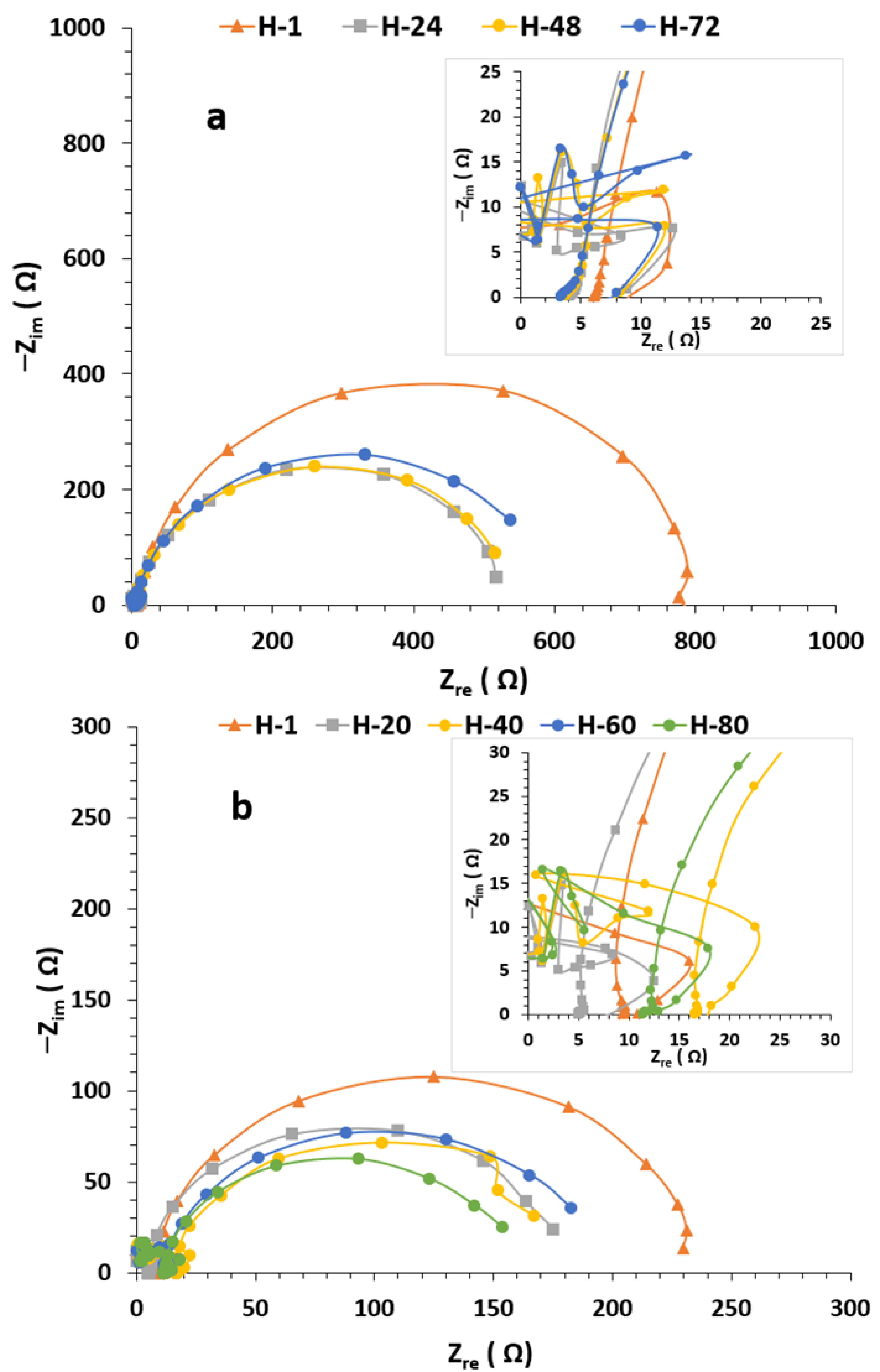
3.4.3. Condition C (O₂ 20%, N₂ 80%)

Figure 15 shows that in the presence of oxygen, there is, in addition to the main loop, a new interface that appears in the low frequencies that could be either a desorption phenomenon that occurs at the interface or a resistance due to the diffusion of oxygen. The analysis of the polarization curves indicates a contribution of diffusion. We are then in a mixed activation–diffusion regime.

Another small capacitive loop appears at very HFs from the beginning of the immersion at 25 °C. It is different from the artifacts encountered for the HF measurements of the other conditions. The associated resistance is initially about 10 ohms and increases regularly at 25 °C. Its diameter increases from 10 to 50 ohms (5 to 12% of the value of the polarization resistance obtained). It is, therefore, attributed to the progressive formation of a layer of corrosion products (iron oxides and hydroxides) in an aerated environment. At 80 °C, the HF loop is absent at the beginning of the immersion, only appears after 48 h, and remains constant until the end of the experiment (the formation of a layer of corrosion products at 80 °C occurs later). At 25 °C, the proposed circuit R(Q(R(Q(RO)))), shown in Figure 16, considers the oxygen diffusion process. The presence of solution agitation results in the existence of a diffuse layer of finite thickness (represented by the O element) instead of a semi-infinite diffusion of type W (Warburg), resulting in the presence of a charge transfer resistance [72].

An acceptable numerical fit (Figure 17 and

Table 6. Results of the impedance simulation obtained under condition C at 25 °C; A = 2 cm².

Circuit Element	Value	Relative Error (%)
Rs (ohms)	2.4	19.4
Yo	1.23 $\times$ 10−5	25.4
nf	0.84	3.7
Rf (ohms)	11	4.8
Ydl	1.83 $\times$ 10−3	1.5
n	0.79	0.6
Rct (ohms)	2155	0.9
O-Yo	0.11	1.1
O-B	11.6	4.2

) is obtained (less than 5% error for the values of Q_dl and R_ct and the O parameters). The value of the thickness of the diffuse layer δ can be calculated using Equation (17):

$$\delta =B_O\times \sqrt{D_{O_2}}$$

(17)

where $B_O$ is a parameter related to the definition of the element O provided by the simulation, and $D_{{\mathrm{O}}_2}=2.1\times {10}^{-5}{\displaystyle \frac{\mathrm{c}{\mathrm{m}}^2}{\mathrm{s}}}$, which is the diffusion coefficient of oxygen at 25 °C. We then find a value of $B_O$ = 11.6 at 12 h, which gives δ = 0.53 mm.

A relatively large value is explainable by low agitation, which occurs far from the working electrode. The calculation of the CCD using the Stern–Geary formula and R_p is not theoretically justified because $R_p\ne R_{ct}$. The Stern–Geary formula here uses $R_{ct}$ [73]. The coefficient n of the Q_dl varies between 0.74 and 0.81 at 25 °C, reflecting significant surface heterogeneity.

At 80 °C, the EEC used at the beginning of the immersion is R(QR(RO)) (shown in Figure 18). It connects the anodic (R_a) and cathodic (R_c) resistances in parallel. The cathodic reaction is limited by diffusion, and the element O is also introduced. In this case, the maximal error is at 11% in the simulation (Figure 19), and the CCD is given by Equation (18).

$$J_{corr}={\displaystyle \frac{{\beta }_a}{2.3\times R_a}}$$

(18)

In Figure 18, R_a is the anodic resistance in Ω·m².

The calculated diffusion layer thickness δ = 0.18 mm is of the same order of magnitude as that noted at 25 °C.

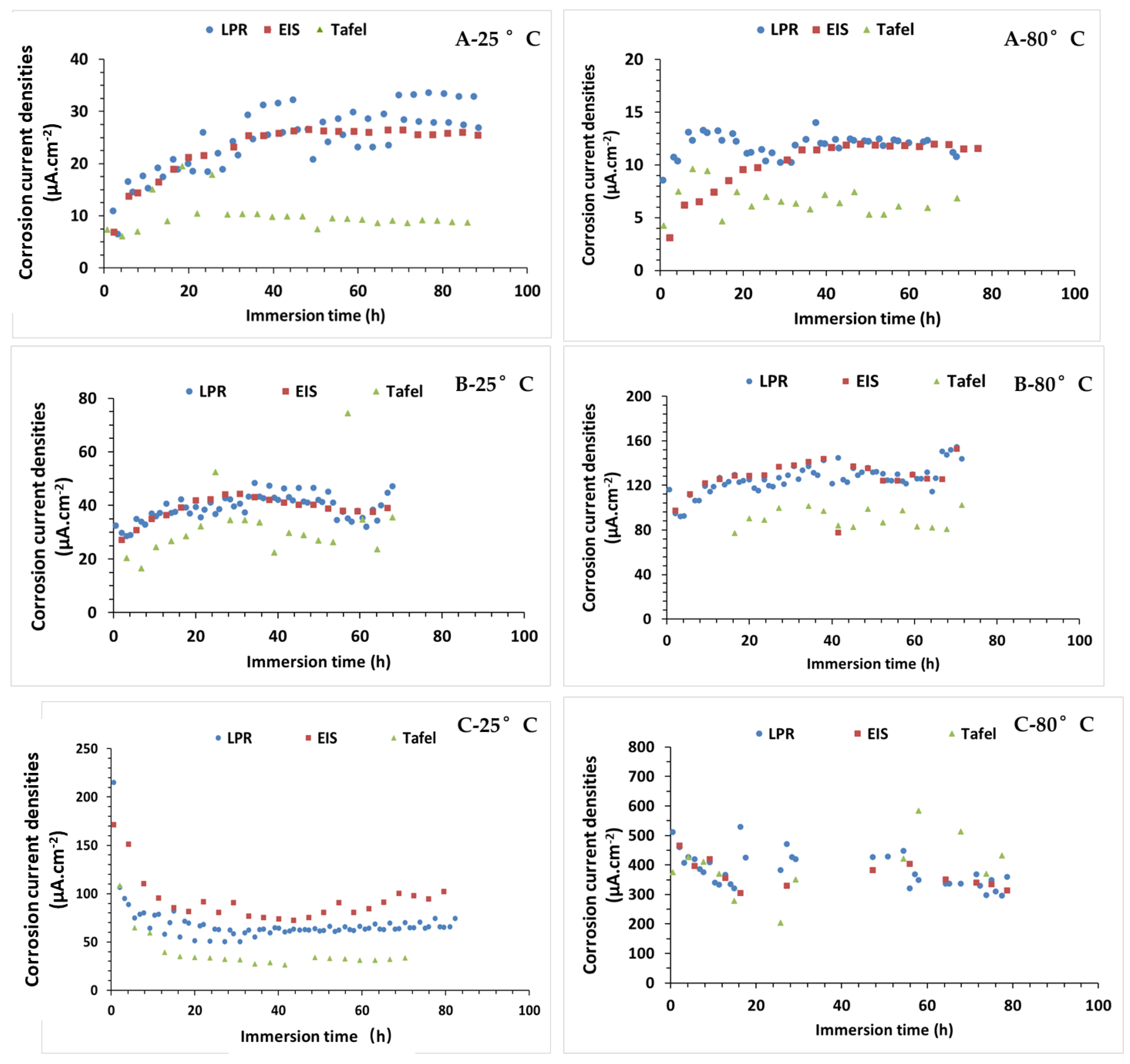
3.5. Corrosion Current Densities (CCD)

Figure 20 presents the comparison of the temporal CCDs estimated from the three methods, including Tafel, LPR, and EIS, under the three conditions at the two temperatures.

Table 7. Comparison of CCD values (µA cm⁻²) obtained with the different techniques for all conditions at 60 h of immersion.

Condition	Corrosion Current Densities (µA cm−2) at 60 h
	LPR	EIS	Tafel
A-CO2 1%, N2 99%; 25 °C	28	25	10
A-CO2 1%, N2 99%; 80 °C	11	32	7
B- H2S 0.8%, CO2 20%, N2 79.2%; 25 °C	43	39	37
B- H2S 0.8%, CO2 20%, N2 79.2%; 80 °C	138	132	103
C-O2 20%, N2 80%; 25 °C	62	81	37
C-O2 20%, N2 80%; 80 °C	236	580	435

summarizes the CCD values at the end of the experiments for the different techniques under the three conditions and the two temperatures.

For LPR, the CCD is calculated using the polarization resistance value, with a parameter B coming from the slopes obtained with the Tafel extrapolation. There is a relatively large intrinsic dispersion with LPR. After the experimental campaign, it was found that some LPR measurements were carried out too close to Tafel measurements such that the steel interface did not sufficiently return to equilibrium.

First, it is observed that the corrosion rates obtained with the three methods (EIS, LPR, and Tafel) are of the same order of magnitude (Figure 20). The values obtained with LPR and EIS show the greatest differences among conditions A-80 °C, C-25 °C, and C-80 °C. In addition to the electronic transfer, a diffusive or capacitive phenomenon appeared that then invalidates the hypothesis of the pure activation regime. In these cases, LPR underestimates the corrosion rate of the steel.

The Tafel method also almost systematically gives lower CCD values (Figure 20). The influence of adsorption phenomena (inductive or capacitive) can be one of the explanations. These phenomena are normally amplified with the increase in anodic polarization. Similarly, the appearance of a diffusion limitation to cathodic overvoltages is known to give, with the Tafel adjustment, lower CCDs [74].

Oxic conditions are the most corrosive (Figure 20C). Indeed, the CCD values obtained are much higher (up to 580 µA cm⁻² or almost 7 mm year⁻¹ of steel thickness consumed). At 25 °C, the drop in CCD initially observed coincides with the appearance of the additional interface identified at HF with the EIS and with the sudden drop in OCP_X65 in the first hours of immersion, reflecting a pseudo-passive effect of the corrosion products.

Then, the presence of H₂S has an accelerating effect on the corrosion kinetics (Figure 20B). No inhibition effect was, moreover, highlighted on the immersion time tested.

The CCD values obtained under condition A (Figure 20A), representative of real Cox water (10–30 µm year⁻¹), are approximately 10 times higher than those we obtained at 25 °C in contact with actual Cox water in another study [18]. The higher rate is partly due to the strong polarization required for the Tafel adjustment, which can initiate steel corrosion in the medium. Indeed, the initial CCD (7 µA cm⁻²), which was obtained before using the Tafel method, is closer to the initial CCDs also obtained in actual Cox water [18]. Temperature clearly has an accelerating effect on steel corrosion under conditions A, B, and C (Figure 20), despite the lower solubility at these temperatures of the oxidizing species H₂S and O₂. Indeed, in the presence of oxygen, the formation of a deposit interface highlighted by EIS at 25 °C is not observed at 80 °C.

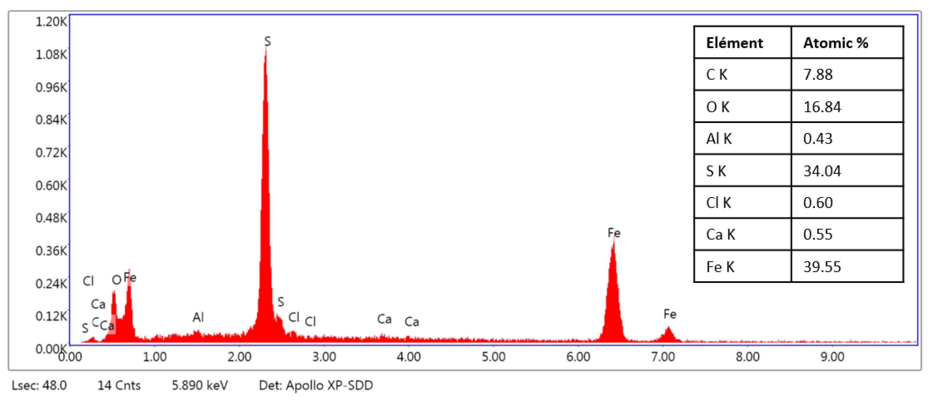
3.6. SEM Characterization of the CS-X65 Surface After Immersion in BM-IRCPW (0.8% H₂S, 20% CO₂, 79.2% N₂) at 80 °C

The SEM analyses performed on CS-X65 allowed for the examination of the steel surface under condition B (presence of sulfides) after more than 70 h of immersion in BM-IRCPW (0.8% H₂S, 20% CO₂, 79.2% N₂) at 80 °C and severe electrochemical disturbances. Figure 21 represents the deterioration of the CS-X65 electrode and the outer layer. Figure 22 presents the EDX analysis, revealing that the steel surface in the outer layer is primarily composed of a mixture of FeS/FeS_1−x.

Figure 23 reveals an ongoing oxidation process of the outer layer in contact with oxygen, despite the precautions taken to minimize this phenomenon during the microscopic observation of the sample.

4. Discussion

The results obtained using LPR and the Tafel method show slight differences compared to those obtained with EIS, although they are of the same order of magnitude. This difference can be explained by the influence of additional processes (charging current during the potentiodynamic polarization) during electrode polarizations [60]. The corrosion rate measured using the Tafel method is consistently lower and further from the value found with the EIS and LPR methods due to a significantly wider polarization range, leading to more pronounced inductive, capacitive, or diffusion effects. Additional phenomena appeared under all conditions, limiting the application of linear polarization methods, such as LPR and the Tafel method.

In Section 2.1.4 we presented the PhreeqC^® simulations of three corrosive solutions, including AM-IRCPW, BM-IRCPW and CM-IRCPW, at both temperatures (in Appendix A, Table A1, Table A2 and Table A3) and in the absence of contact with carbon steel. These tables are useful because they contain the saturation of the main phases in each case. Table A4, Table A5 and Table A6 present the main changes in the saturation of the main phases after considering the presence of a dissolved iron content, assumed to come from corrosion and 10 times higher than that of the IRCPW. After the experiments, these simulations permit comparisons of the results of the evolution/interactions in these waters in the absence and presence of carbon steel.

In bubbling with CO₂ (condition A), the corrosion of steel can be broken down into three stages:

-

The first stage involves the initiation of the steel corrosion with co-adsorption of hydrogen, chloride, and bicarbonate atoms from the first hours of immersion of the steel. The adsorption is clearly visible at low frequencies on the Nyquist plots.

-

The second stage involves the formation of deposits of non-crystallized iron carbonates on the surface of the steel at 25 °C and especially at 80 °C (see Table A1 and Table A4). These rather protective deposits do not completely cover the surface of the steel and have the particularity of polarizing the steel. EIS also highlights this based on the appearance in high frequencies of a new interface after a couple of hours.

-

The last stage corresponds to the progressive crystallization of iron carbonate deposits into siderite (FeCO₃) at 80 °C. This change in the structure of the deposits leads to a relative ennoblement of the carbon steel over time. The polarization resistances at 80 °C are low, but not much lower at 80 °C than at 25 °C. This shows the partially protective effect of siderite deposits, which are much greater at 80 °C [35] and compensate for the higher corrosiveness of the fluid at this temperature.

All these mechanisms are perfectly enhanced by the behavior of the electrodes where the three stages are distinguished (with LPR and Tafel methods) during the immersion where the second and third stages are much slower at 25 °C than at 80 °C. The same corrosion products (iron carbonates) have been found when studying the corrosion of carbon steels in direct contact with Cox water [12,13,14], with lower corrosion rates, using non-destructive measurement methods over longer exposure times.

By bubbling with sulfide and CO₂ (condition B), we have also three different stages of iron dissolution:

-

The initiation of the steel corrosion with co-adsorption of hydrogen and sulfide during occurs the first hours of immersion of the steel. This results in a reduction and thus maintenance at a constant value of the corrosion rate of the steel.

-

The second stage involves the formation of iron sulfide deposits on the surface of the steel (see Table A2 and Table A5), which also slightly polarize the steel. In this case, we transition from a first type electrode to a second type electrode (Fe/FeS/S²⁻) for iron oxidation. The solution quickly darkens due to the formation of large quantities of iron sulfides (availability of Fe²⁺ due to polarization at 200 mV/OCP) and sulfides.

-

The last phase corresponds to the progressive crystallization of sulfide deposits from the FeS form to the Fe_xS_y form [16]. In presence of small amount of sulfides due to H₂ production from corrosion and microbial activity, magnetite was observed in Cox water, while denser pyrite was found at 90 °C in relatively long term experiments (3 months) [16]. In this case, the pyrite formation at 90 °C inhibits the corrosion reaction. In our short-term and electrochemically aggressive experiment, with a CO₂/H₂S ratio of 25, mackinawite (FeS), which is weakly protective, is indeed the main corrosion product formed at 25 °C. The solubility of H₂S is lower at 80 °C than at 25 °C, as highlighted in the PhreeqC simulations. However, FeS deposits, which are electroactive, become more reactive at higher temperatures, leading to an acceleration of corrosion at elevated temperatures. Furthermore, for pH values between 4 and 5.5, FeS protective films are unstable and partially dissolve, exposing carbon steel to a faster uniform attack [75]. The presence of iron sulfides is clearly evidenced. Unlike condition A, which does not contain sulfides, siderite (FeCO₃) precipitation is unstable in the presence of sulfides. Even at 80 °C [75], where siderite normally forms in greater amounts, it remains a minor phase. At 80 °C, mackinawite transforms into more crystalline phases. However, due to their fissured and fragile nature, they promote localized corrosion, which can further accelerate the overall corrosion process. The progressive increase and transformation of amorphous FeS into crystalline, conductive mackinawite (pyrrhotite and pyrite in actual geothermal waters) leads to a continuous and severe attack on carbon steel [48].

In bubbling with O₂ and N₂ (condition C), the corrosion of steel can be broken down into two stages:

-

The first stage involves the initiation of the steel corrosion. The O₂ is available, and the corrosion rate is initially very high (hundreds of µA/cm² at this stage).

-

The second stage involves the formation of corrosion deposits at the steel surface highlighted by the EIS in both cases (25 °C and 80 °C). This is correlated with a drop in corrosion rate measurements. Note that the appearance of the deposit using the EIS diagram at 80 °C occurred after 48 h of immersion, whereas it occurred in the first hours at 25 °C. With the PhreeqC simulations made (see Table A3 and Table A6), the corrosion products expected in these cases (large presence of oxygen) are ferrous oxides (magnetite and hematite) at 25 °C. At 80 °C, hematite is expected, but with a much lower SI (3.83 at 80 °C versus 14.7 at 25 °C), and no magnetite, consistent with the latter appearance of a new interface at the steel surface in the high temperature experiment (80 °C).

The most corrosive conditions exhibit the following order: C at 80 °C, B at 80 °C, C at 25 °C, B at 25 °C, A at 80 °C, and A at 25 °C. The corrosion rates are the lowest for bubbling with atmosphere A (pCO₂ = 0.01 atm), which mimics the pore water of Cox, when it is not disturbed either by bacterial activity or by oxygen ingress.

5. Conclusions

The corrosion experiments we conducted with API 5L X65 steel in contact with synthetic Cox water and specific atmospheres allowed us to deepen in a short period of time our understanding of the influence of various gases (oxygen, sulfide, and carbon dioxide) on corrosion kinetics, as well as in aqueous environments. The corrosion rates obtained in the first few hours while bubbling under condition A (CO₂ 1%, N₂ 99%), which is the closest to real conditions, are consistent with the corrosion rates of steel in contact with natural pore water [18] that we obtained earlier. The ’destructive’ methods applied afterwards explain the difference.

In this anoxic environment, the interfacial phenomena of steel mainly involve the combination of charge transfer associated with double-layer capacitance. However, significant adsorption caused by Cl^- and H⁺ ions occurs during the first few hours of immersion but gradually decreases over time. The observed adsorption is more significant at 25 °C than at 80 °C, as adsorption is an exothermic process naturally favored at lower temperatures. By the end of the experiment (72–96 h), a pseudo-capacitive phenomenon appears at low frequencies, attributed to the relaxation of corrosion products, which are rather conductive and non-protective, leading to a sharp increase in interfacial capacitance. The measured corrosion rate is around 100–300 µm year⁻¹.

In the presence of sulfides and a higher amount of carbon dioxide (atmosphere B: 0.8% H₂S, 20% CO₂, 79.2% N₂), the pH of the solution drops, going from a value of 6 under condition A to 4–4.5. The adsorption effects of H₂S were observed during the first hours of immersion. Sulfides accelerate the corrosion rate of steel, especially at higher temperatures. Corrosion is around 400 µm year⁻¹ at 25 °C and greater (1–1.5 mm year⁻¹) at 80 °C.

With air bubbling, corrosion rates are initially very high, reaching up to 7 mm year⁻¹ at 80 °C and 1.8 mm year⁻¹ at 25 °C in the first few hours. Then, pseudo-passivity is observed on the EIS diagrams at 25 °C, slowing the corrosion rate to less than 1 mm/year. The process is characterized by corrosion control through oxygen diffusion, with the boundary layer thickness estimated at around 0.5 mm.

References

1. Altmann, S. ’Geo’chemical Research: A Key Building Block for Nuclear Waste Disposal Safety Cases. J. Contam. Hydrol. 2008, 102, 174–179. [Google Scholar] [CrossRef] [PubMed]
2. Han, T.; Shi, J.; Chen, Y.; Li, Z. Effect of Chemical Corrosion on the Mechanical Characteristics of Parent Rocks for Nuclear Waste Storage. Sci. Technol. Nucl. Install. 2016, 2016, 7853787. [Google Scholar] [CrossRef]
3. Jonsson, M. Radiation Effects on Materials Used in Geological Repositories for Spent Nuclear Fuel. Int. Sch. Res. Not. 2012, 2012, 639520. [Google Scholar] [CrossRef]
4. Gaucher, E.; Robelin, C.; Matray, J.M.; Négrel, G.; Gros, Y.; Heitz, J.F.; Vinsot, A.; Rebours, H.; Cassagnabère, A.; Bouchet, A. ANDRA Underground Research Laboratory: Interpretation of the Mineralogical and Geochemical Data Acquired in the Callovian–Oxfordian Formation by Investigative Drilling. Phys. Chem. Earth Parts A/B/C 2004, 29, 55–77. [Google Scholar] [CrossRef]
5. Gaucher, É.C.; Blanc, P.; Bardot, F.; Braibant, G.; Buschaert, S.; Crouzet, C.; Gautier, A.; Girard, J.-P.; Jacquot, E.; Lassin, A.; et al. Modelling the porewater chemistry of the Callovian–Oxfordian formation at a regional scale. Comptes Rendus. Géoscience 2006, 338, 917–930. [Google Scholar] [CrossRef]
6. Gaucher, E.C.; Tournassat, C.; Pearson, F.J.; Blanc, P.; Crouzet, C.; Lerouge, C.; Altmann, S. A Robust Model for Pore-Water Chemistry of Clayrock. Geochim. Cosmochim. Acta 2009, 73, 6470–6487. [Google Scholar] [CrossRef]
7. Fernández, A.M.; Sánchez-Ledesma, D.M.; Tournassat, C.; Melón, A.; Gaucher, E.C.; Astudillo, J.; Vinsot, A. Applying the Squeezing Technique to Highly Consolidated Clayrocks for Pore Water Characterisation: Lessons Learned from Experiments at the Mont Terri Rock Laboratory. Appl. Geochem. 2014, 49, 2–21. [Google Scholar] [CrossRef]
8. Tournassat, C.; Bourg, I.C.; Steefel, C.I.; Bergaya, F. Chapter 1—Surface Properties of Clay Minerals. In Developments in Clay Science; Tournassat, C., Steefel, C.I., Bourg, I.C., Bergaya, F., Eds.; Natural and Engineered Clay Barriers; Elsevier: Amsterdam, The Netherlands, 2015; Volume 6, pp. 5–31. [Google Scholar]
9. Vinsot, A.; Appelo, C.A.J.; Cailteau, C.; Wechner, S.; Pironon, J.; De Donato, P.; De Cannière, P.; Mettler, S.; Wersin, P.; Gäbler, H.-E. CO2 Data on Gas and Pore Water Sampled in Situ in the Opalinus Clay at the Mont Terri Rock Laboratory. Phys. Chem. Earth Parts A/B/C 2008, 33, S54–S60. [Google Scholar] [CrossRef]
10. Vinsot, A.; Mettler, S.; Wechner, S. In Situ Characterization of the Callovo-Oxfordian Pore Water Composition. Phys. Chem. Earth Parts A/B/C 2008, 33, S75–S86. [Google Scholar] [CrossRef]
11. Martin, F.A.; Perrin, S.; Bataillon, C. Evaluating the Corrosion Rate of Low Alloyed Steel in Callovo-Oxfordian Clay: Towards a Complementary EIS, Gravimetric and Structural Study. MRS Online Proc. Libr. 2012, 1475, 471–476. [Google Scholar] [CrossRef]
12. Schlegel, M.L.; Necib, S.; Daumas, S.; Blanc, C.; Foy, E.; Trcera, N.; Romaine, A. Microstructural Characterization of Carbon Steel Corrosion in Clay Borehole Water under Anoxic and Transient Acidic Conditions. Corros. Sci. 2016, 109, 126–144. [Google Scholar] [CrossRef]
13. Necib, S.; Linard, Y.; Crusset, D.; Schlegel, M.; Daumas, S.; Michau, N. Corrosion Processes of C-Steel in Long-Term Repository Conditions. Corros. Eng. Sci. Technol. 2017, 52, 127–130. [Google Scholar] [CrossRef]
14. Necib, S.; Linard, Y.; Crusset, D.; Michau, N.; Daumas, S.; Burger, E.; Romaine, A.; Schlegel, M.L. Corrosion at the Carbon Steel–clay Borehole Water and Gas Interfaces at 85 °C under Anoxic and Transient Acidic Conditions. Corros. Sci. 2016, 111, 242–258. [Google Scholar] [CrossRef]
15. Hajj, H.E.; Abdelouas, A.; Grambow, B.; Martin, C.; Dion, M. Microbial Corrosion of P235GH Steel under Geological Conditions. Phys. Chem. Earth Parts A/B/C 2010, 35, 248–253. [Google Scholar] [CrossRef]
16. Mendili, Y.E.; Abdelouas, A. Corrosion of P235GH Carbon Steel in Simulated Bure Soil Solution. J. Mater. Environ. Sci 2013, 4, 786–791. [Google Scholar]
17. El Mendili, Y.; Abdelouas, A.; Karakurt, G.; Aït Chaou, A.; Essehli, R.; Bardeau, J.-F.; Grenèche, J.-M. The Effect of Temperature on Carbon Steel Corrosion under Geological Conditions. Appl. Geochem. 2015, 52, 76–85. [Google Scholar] [CrossRef]
18. Sano Moyeme, Y.C.; Betelu, S.; Bertrand, J.; Groenen Serrano, K.; Ignatiadis, I. Corrosion Current Density of API 5L X65 Carbon Steel in Contact with Natural Callovian-Oxfordian Clay Pore Water, Assessed by Various Electrochemical Methods over 180 Days. Metals 2023, 13, 966. [Google Scholar] [CrossRef]
19. Lotz, H.; Neff, D.; Mercier-Bion, F.; Bataillon, C.; Dillmann, P.; Gardés, E.; Monnet, I.; Dynes, J.J.; Foy, E. Localised Corrosion of Iron and Steel in the Callovo-Oxfordian Porewater after 3 Months at 120 C: Characterizations at Micro and Nanoscale and Formation Mechanisms. Corros. Sci. 2023, 219, 111235. [Google Scholar] [CrossRef]
20. Comeaux, R.V. The Role of Oxygen in Corrosion and Cathodic Protection. Corrosion 1952, 8, 305–310. [Google Scholar] [CrossRef]
21. Ruther, W.E.; Hart, R.K. Influence of Oxygen on High Temperature Aqueous Corrosion of Iron. Corrosion 1963, 19, UAC-6956. [Google Scholar] [CrossRef]
22. Strauss, M.B.; Bloom, M.C. Corrosion Mechanisms in the Reaction of Steel with Water and Oxygenated Solutions at Room Temperature and 316 °C. J. Electrochem. Soc. 1960, 107, 73. [Google Scholar] [CrossRef]
23. Cox, G.L.; Roetheli, B.E. Effect of Oxygen Concentration on Corrosion Rates of Steel and Composition of Corrosion Products Formed in Oxygenated Water. Ind. Eng. Chem. 1931, 23, 1012–1016. [Google Scholar] [CrossRef]
24. Tromans, D. Modeling Oxygen-Controlled Corrosion of Steels in Hot Waters. Corrosion 1999, 55, 942–947. [Google Scholar] [CrossRef]
25. Huang, Y.H.; Zhang, T.C. Effects of Dissolved Oxygen on Formation of Corrosion Products and Concomitant Oxygen and Nitrate Reduction in Zero-Valent Iron Systems with or without Aqueous Fe2+. Water Res. 2005, 39, 1751–1760. [Google Scholar] [CrossRef]
26. El Hajj, H.; Abdelouas, A.; El Mendili, Y.; Karakurt, G.; Grambow, B.; Martin, C. Corrosion of Carbon Steel under Sequential Aerobic–Anaerobic Environmental Conditions. Corros. Sci. 2013, 76, 432–440. [Google Scholar] [CrossRef]
27. Saha, J.K. Corrosion of Constructional Steels in Marine and Industrial Environment: Frontier Work in Atmospheric Corrosion; Engineering Materials; Springer: Chennai, India, 2013; ISBN 978-81-322-0719-1. [Google Scholar]
28. Lu, W.-F.; Chen, T.-C.; Tsai, K.-C.; Yung, T.-Y. The Corrosion Behavior of Carbon Steel Materials Used at Nuclear Power Plants During Deactivation and Decommissioning Processes. Metals 2024, 14, 1444. [Google Scholar] [CrossRef]
29. Tran, T.; Brown, B.; Nesic, S. Corrosion of Mild Steel in an Aqueous CO2 Environment–Basic Electrochemical Mechanisms Revisited. In Corrosion Conference and Expo 2015, Proceedings of the Nace Corrosion, Dallas, TX, USA, 5–19 March 2015; NACE: Houston, TX, USA, 2015; p. NACE-2015. [Google Scholar]
30. Basilico, E.; Marcelin, S.; Mingant, R.; Kittel, J.; Fregonese, M.; Ropital, F. The Effect of Chemical Species on the Electrochemical Reactions and Corrosion Product Layer of Carbon Steel in CO2 Aqueous Environment: A Review. Mater. Corros. 2021, 72, 1152–1167. [Google Scholar] [CrossRef]
31. Shayegani, M.; Afshar, A.; Ghorbani, M.; Rahmaniyan, M. Mild Steel Carbon Dioxide Corrosion Modelling in Aqueous Solutions. Corros. Eng. Sci. Technol. 2008, 43, 290–296. [Google Scholar] [CrossRef]
32. Ogundele, G.I.; White, W.E. Some Observations on Corrosion of Carbon Steel in Aqueous Environments Containing Carbon Dioxide. Corrosion 1986, 42, 71–78. [Google Scholar] [CrossRef]
33. Yang, S.; Li, M.; Liu, T.; Gao, P.; Zhang, H.; Yin, C.; Tang, Y. Protective Mechanism of Carbon Dioxide in Pipelines for Water Containing Typical Corrosive Anions. Process Saf. Environ. Prot. 2024, 188, 654–663. [Google Scholar] [CrossRef]
34. Refait, P.; Grolleau, A.-M.; Jeannin, M.; Rémazeilles, C.; Sabot, R. Corrosion of Carbon Steel in Marine Environments: Role of the Corrosion Product Layer. Corros. Mater. Degrad. 2020, 1, 198–218. [Google Scholar] [CrossRef]
35. Taleb, W.; Pessu, F.; Wang, C.; Charpentier, T.; Barker, R.; Neville, A. Siderite Micro-Modification for Enhanced Corrosion Protection. npj Mater. Degrad. 2017, 1, 1–6. [Google Scholar] [CrossRef]
36. da Silva, P.N.; Dugstad, A.; Svenningsen, G.; da Cunha Ponciano Gomes, J.A. The Influence of Oxygen on Protective Iron Carbonate Scales Formed on Carbon Steel in CO2 Environments at Near-Neutral pH. In Proceedings of the AMPP Annual Conference + Expo, San Antonio, TX, USA, 6 March 2022. [Google Scholar]
37. Ma, H.; Cheng, X.; Li, G.; Chen, S.; Quan, Z.; Zhao, S.; Niu, L. The Influence of Hydrogen Sulfide on Corrosion of Iron under Different Conditions. Corros. Sci. 2000, 42, 1669–1683. [Google Scholar] [CrossRef]
38. Gao, S.; Brown, B.; Young, D.; Nesic, S.; Singer, M. Formation Mechanisms of Iron Oxide and Iron Sulfide at High Temperature in Aqueous H2S Corrosion Environment. J. Electrochem. Soc. 2018, 165, C171. [Google Scholar] [CrossRef]
39. Cheng, X.L.; Ma, H.Y.; Zhang, J.P.; Chen, X.; Chen, S.H.; Yang, H.Q. Corrosion of Iron in Acid Solutions with Hydrogen Sulfide. Corrosion 1998, 54, 369–376. [Google Scholar] [CrossRef]
40. Yoo, J.-S.; Chung, N.T.; Lee, Y.-H.; Kim, Y.-W.; Kim, J.-G. Effect of Sulfide and Chloride Ions on Pitting Corrosion of Type 316 Austenitic Stainless Steel in Groundwater Conditions Using Response Surface Methodology. Materials 2024, 17, 178. [Google Scholar] [CrossRef]
41. Ma, H.; Cheng, X.; Chen, S.; Wang, C.; Zhang, J.; Yang, H. An Ac Impedance Study of the Anodic Dissolution of Iron in Sulfuric Acid Solutions Containing Hydrogen Sulfide. J. Electroanal. Chem. 1998, 451, 11–17. [Google Scholar] [CrossRef]
42. Romaine, A. Role of Sulfide Species in the Corrosion of Non-Alloy Steel: Heterogeneities of the Layer of Corrosion Products and Galvanic Coupling. Ph.D. Thesis, Universiy of La Rochelle, La Rochelle, France, 2014. [Google Scholar]
43. Somervuori, M.; Isotahdon, E.; Nuppunen-Puputti, M.; Bomberg, M.; Carpén, L.; Rajala, P. A Comparison of Different Natural Groundwaters from Repository Sites—Corrosivity, Chemistry and Microbial Community. Corros. Mater. Degrad. 2021, 2, 603–624. [Google Scholar] [CrossRef]
44. Konovalova, V. The Effect of Temperature on the Corrosion Rate of Iron-Carbon Alloys. Mater. Today: Proc. 2021, 38, 1326–1329. [Google Scholar] [CrossRef]
45. Betelu, S.; Tournassat, C.; Bertrand, J.; Ignatiadis, I. Pyrite-Electrode Potential Measurements in Reference Solutions versus Measured and Computed Redox Potential: At the Roots of an Innovative Generic pH Electrode for Nuclear Waste Repositories. In Proceedings of the 12th International High-Level Radioactive Waste Management Conference, Albuquerque, NM, USA, 29 April–3 May 2012. [Google Scholar]
46. Blanc, P.; Lassin, A.; Piantone, P.; Azaroual, M.; Jacquemet, N.; Fabbri, A.; Gaucher, E.C. Thermoddem: A Geochemical Database Focused on Low Temperature Water/Rock Interactions and Waste Materials. Appl. Geochem. 2012, 27, 2107–2116. [Google Scholar] [CrossRef]
47. Castillo, C.; Ignatiadis, I. Sulfate-Reduction State of the Geothermal Dogger Aquifer, Paris Basin, France After 35 Years of Exploitation: Analysis And Consequences of Bacterial Proliferation in Casings and Reservoir. In Proceedings of the Thirty-Seventh Workshop on Geothermal Reservoir Engineering, Stanford, CA, USA, 30 January–1 February 2012. [Google Scholar]
48. Betelu, S.; Helali, C.; Ignatiadis, I. Laboratory-Scale Implementation of Standardized Reconstituted Geothermal Water for Electrochemical Investigations of Carbon Steel Corrosion. Metals 2024, 14, 1216. [Google Scholar] [CrossRef]
49. Gabrielli, C.; Takenouti, H. Méthodes Électrochimiques Appliquées à La Corrosion-Techniques Dynamiques. Les Tech. L’ingenieur 2010, COR 811, 1–22. [Google Scholar] [CrossRef]
50. Reeve, J.C.; Bech-Nielsen, G. The Stern-Geary Method. Basic Difficulties and Limitations and a Simple Extension Providing Improved Reliability. Corros. Sci. 1973, 13, 351–359. [Google Scholar] [CrossRef]
51. Angst, U.; Büchler, M. On the Applicability of the Stern–Geary Relationship to Determine Instantaneous Corrosion Rates in Macro-Cell Corrosion. Mater. Corros. 2015, 66, 1017–1028. [Google Scholar] [CrossRef]
52. Mansfeld, F.; Oldham, K.B. A Modification of the Stern—Geary Linear Polarization Equation. Corros. Sci. 1971, 11, 787–796. [Google Scholar] [CrossRef]
53. Bard, A.J.; Faulkner, L.R. Electrochemical Methods: Fundamentals and Applications. Surf. Technol. 1983, 20, 91–92. [Google Scholar]
54. Panchenko, Y.M.; Marshakov, A.I.; Igonin, T.N.; Kovtanyuk, V.V.; Nikolaeva, L.A. Long-Term Forecast of Corrosion Mass Losses of Technically Important Metals in Various World Regions Using a Power Function. Corros. Sci. 2014, 88, 306–316. [Google Scholar] [CrossRef]
55. Jiao, D.; Rempe, S.B. CO2 Solvation Free Energy Using Quasi-Chemical Theory. J. Chem. Phys. 2011, 134, 224506. [Google Scholar] [CrossRef]
56. Duan, Z.; Sun, R.; Liu, R.; Zhu, C. Accurate Thermodynamic Model for the Calculation of H2S Solubility in Pure Water and Brines. Energy Fuels 2007, 21, 2056–2065. [Google Scholar] [CrossRef]
57. Daoudi, J.; Betelu, S.; Tzedakis, T.; Bertrand, J.; Ignatiadis, I. A Multi-Parametric Device with Innovative Solid Electrodes for Long-Term Monitoring of pH, Redox-Potential and Conductivity in a Nuclear Waste Repository. Sensors 2017, 17, 1372. [Google Scholar] [CrossRef] [PubMed]
58. Boyd, C.E. Boyd, C.E., Ed.; Dissolved Oxygen and Redox Potential. In Water Quality: An Introduction; Springer: Boston, MA, USA, 2000; pp. 69–94. ISBN 978-1-4615-4485-2. [Google Scholar]
59. Aslam, R. Chapter 2—Potentiodynamic Polarization Methods for Corrosion Measurement. In Electrochemical and Analytical Techniques for Sustainable Corrosion Monitoring; Aslam, J., Verma, C., Mustansar Hussain, C., Eds.; Elsevier: Amsterdam, The Netherlands, 2023; pp. 25–37. ISBN 978-0-443-15783-7. [Google Scholar]
60. Zhang, X.L.; Jiang, Z.H.; Yao, Z.P.; Song, Y.; Wu, Z.D. Effects of Scan Rate on the Potentiodynamic Polarization Curve Obtained to Determine the Tafel Slopes and Corrosion Current Density. Corros. Sci. 2009, 51, 581–587. [Google Scholar] [CrossRef]
61. Zhou, H.; Chhin, D.; Morel, A.; Gallant, D.; Mauzeroll, J. Potentiodynamic Polarization Curves of AA7075 at High Scan Rates Interpreted Using the High Field Model. npj Mater. Degrad. 2022, 6, 1–11. [Google Scholar] [CrossRef]
62. Frankel, G.S. Hughes, A.E., Mol, J.M.C., Zheludkevich, M.L., Buchheit, R.G., Eds.; Fundamentals of Corrosion Kinetics. In Active Protective Coatings; Springer Series in Materials Science; Springer: Dordrecht, The Netherlands, 2016; Volume 233, pp. 17–32. ISBN 978-94-017-7538-0. [Google Scholar]
63. Poorqasemi, E.; Abootalebi, O.; Peikari, M.; Haqdar, F. Investigating Accuracy of the Tafel Extrapolation Method in HCl Solutions. Corros. Sci. 2009, 51, 1043–1054. [Google Scholar] [CrossRef]
64. De Oliveira, M.C.; Figueredo, R.M.; Acciari, H.A.; Codaro, E.N. Corrosion Behavior of API 5L X65 Steel Subject to Plastic Deformation. J. Mater. Res. Technol. 2018, 7, 314–318. [Google Scholar] [CrossRef]
65. Zhang, R.; Sur, D.; Li, K.; Witt, J.; Black, R.; Whittingham, A.; Scully, J.R.; Hattrick-Simpers, J. Bayesian Assessment of Commonly Used Equivalent Circuit Models for Corrosion Analysis in Electrochemical Impedance Spectroscopy. npj Mater. Degrad. 2024, 8, 1–7. [Google Scholar] [CrossRef]
66. McCafferty, E.; Hackerman, N. Double Layer Capacitance of Iron and Corrosion Inhibition with Polymethylene Diamines. J. Electrochem. Soc. 1972, 119, 146. [Google Scholar] [CrossRef]
67. Bonnel, A.; Dabosi, F.; Deslouis, C.; Duprat, M.; Keddam, M.; Tribollet, B. Corrosion Study of a Carbon Steel in Neutral Chloride Solutions by Impedance Techniques. J. Electrochem. Soc. 1983, 130, 753. [Google Scholar] [CrossRef]
68. Guo, X.-P.; Tomoe, Y. The Effect of Corrosion Product Layers on the Anodic and Cathodic Reactions of Carbon Steel in CO2-Saturated Mdea Solutions at 100 °C. Corros. Sci. 1999, 41, 1391–1402. [Google Scholar] [CrossRef]
69. Flis, J.; Dawson, J.L.; Gill, J.; Wood, G.C. Impedance and Electrochemical Noise Measurements on Iron and Iron-Carbon Alloys in Hot Caustic Soda. Corros. Sci. 1991, 32, 877–892. [Google Scholar] [CrossRef]
70. Christensen, B.J.; Mason, T.O.; Jennings, H.M. Influence of Silica Fume on the Early Hydration of Portland Cements Using Impedance Spectroscopy. J. Am. Ceram. Soc. 1992, 75, 939–945. [Google Scholar] [CrossRef]
71. Ma, H.Y.; Cheng, X.L.; Chen, S.H.; Li, G.Q.; Chen, X.; Lei, S.B.; Yang, H.Q. Theoretical Interpretation on Impedance Spectra for Anodic Iron Dissolution in Acidic Solutions Containing Hydrogen Sulfide. Corrosion 1998, 54, 634–640. [Google Scholar] [CrossRef]
72. Mansfeld, F. Discussion: Electrochemical Techniques for Studying Corrosion of Reinforcing Steel: Limitations and Advantages. Corrosion 2005, 61, 739–742. [Google Scholar] [CrossRef]
73. Epelboin, I.; Gabrielli, C.; Keddam, M.; Takenouti, H. The Study of the Passivation Process by the Electrode Impedance Analysis. In Electrochemical Materials Science; Bockris, J.O., Conway, B.E., Yeager, E., White, R.E., Eds.; Springer: Boston, MA, USA, 1981; pp. 151–192. ISBN 978-1-4757-4827-7. [Google Scholar]
74. El-Feki, A.A.; Walter, G.W. Corrosion Rate Measurements under Conditions of Mixed Charge Transfer plus Diffusion Control Including the Cathodic Metal Ion Deposition Partial Reaction. Corros. Sci. 2000, 42, 1055–1070. [Google Scholar] [CrossRef]
75. Choi, Y.-S.; Hassani, S.; Vu, T.N.; Nešić, S.B.; Abas, A.Z.; Nor, A.M.; Suhor, M.F. Strategies for Corrosion Inhibition of Carbon Steel Pipelines Under Supercritical CO2/H2S Environments. Corrosion 2019, 75, 1156–1172. [Google Scholar] [CrossRef]
Figure 1. (A) Photographs of the CS-X65 working electrode and its parts; (B) zoomed image of the dimensions and the lateral cylindrical exposed surface. The electrode dimensions were 7 mm diameter and 9 mm height, with an exposed surface of 2 cm2.
Metals 15 00221 g001
Figure 3. Schematic representation of an electrochemical analysis loop carried out on CS-X65 samples; duration, ~3 h 55 min. SEcorr: monitoring of EX65, the open circuit potential of CS-X65; SJcorr: potentiostatic technique at EX65 with monitoring of corrosion free-current density Jcorr at the EX65; LRP: monitoring of Rp, allowing access to Jcorr; TP: monitoring of EX65, Jcorr, βa, and βc; EIS at EX65: monitoring of the X65 corrosion mechanism, monitoring of Rp, allowing access to Jcorr. Arrows show the end of one technique and the beginning of the next, the number associated at a technique name corresponds to the number of times the technique is performed.
Metals 15 00221 g003
Figure 4. Redox potential and pH of IRCPW at 25 °C and 80 °C, under different conditions: (A) CO2 1%, N2 99%; (B) H2S 0.8%, CO2 20%, N2 79.2%; and (C) O2 20%, N2 80%.
Metals 15 00221 g004
Figure 5. Temporal variations in EX65 or OCPX65 (in mV/SCE) at 25 °C and 80 °C under different conditions (A: CO2 1%, N2 99%; B: H2S 0.8%, CO2 20%, N2 79.2%; and C: O2 20%, N2 80%).
Metals 15 00221 g005
Figure 6. Polarization curves obtained with CS-X65 in IRCPW with bubbling of a gas composed of 99% N2 and 1% CO2. (a) 25 °C, (b) 80 °C. H-1 means first hour of measurement. E ranges from −200 mV/OCPX65 to +200 mV/OCPX65.
Metals 15 00221 g006
Figure 7. Tafel curves of the three different bubbling conditions at 25 °C and 80 °C after 48 h (sufficient time to consider a stabilization).
Metals 15 00221 g007
Figure 8. Time evolution of impedances in the Nyquist plane under condition A at 25 °C (CO2 1%, N2 99%); A = 2 cm2.
Metals 15 00221 g008
Figure 9. The equivalent electrical circuit (EEC) considering induction at low frequencies under condition A at 25 °C (CO2 1%, N2 99%); A = 2 cm2.
Metals 15 00221 g009
Figure 10. Simulation at 24 h under condition A at 25 °C: (a) Nyquist mode; (b) Bode mode; A = 2 cm2.
Metals 15 00221 g010
Figure 11. Evolution of the double layer capacity (Cdl) and the dispersion coefficient as a function of time under condition A at 25 °C (CO2 1%, N2 99%).
Metals 15 00221 g011
Figure 12. Time evolution of impedances in the Nyquist plane under condition A at 80 °C (CO2 1%, N2 99); A = 2 cm2.
Metals 15 00221 g012
Figure 13. (a) Simulation performed at 1 h under condition A at 80 °C in the Bode diagram; (b) EEC taking into account an additional pseudo-capacitance and simulation results.
Metals 15 00221 g013
Figure 14. Temporal evolution of impedances in the Nyquist plane under condition B (H2S 0.8%, CO2 20%, N2 79.2%) at (a) 25 °C; (b) 80 °C.
Metals 15 00221 g014
Figure 15. Temporal evolution of impedances in the Nyquist plane under condition C (O2 20%, N2 80%) at (a) 25 °C, (b) 80 °C; A = 2 cm2.
Metals 15 00221 g015
Figure 16. The EEC, R(Q(R(Q(RO))), used to model the interface under condition C (CO2 20%, N2 80%) at 25 °C.
Metals 15 00221 g016
Figure 17. Simulation carried out at 12 h under condition C at 25 °C represented in a Nyquist diagram; A = 2 cm2.
Metals 15 00221 g017
Figure 18. The EEC, R(QR(RO)), used to model the interface under condition C (CO2 20%, N2 80%) at 80 °C.
Metals 15 00221 g018
Figure 19. Simulation carried out at 1 h under condition C at 80 °C presented in a Nyquist diagram; A = 2 cm2.
Metals 15 00221 g019
Figure 20. Temporal variation in corrosion current densities (CCDs) under conditions (AC) and at two temperatures with three electrochemical techniques: LPR, EIS, and Tafel.
Metals 15 00221 g020
Figure 21. SEM–EDX analyses carried out on the CS-X65 electrode that was immersed in BM-IRCPW at 80 °C and disturbed for 70 h. L1 is the thickness of the deposit.
Metals 15 00221 g021
Figure 22. SEM–EDX analyses carried out on the CS-X65 electrode that was immersed in BM-IRCPW at 80 °C and disturbed for 70 h.
Metals 15 00221 g022
Figure 23. Zoomed image the external surface of the scale coated on the CS-X65 electrode BM-IRCPW at 80 °C and disturbed for 70 h.
Metals 15 00221 g023