Article

Synthetic Rebalancing of Imbalanced Macro Etch Testing Data for Deep Learning Image Classification

by
Yann Niklas Schöbel
1,2,*,
Martin Müller
2,3 and
Frank Mücklich
2,3
1
Materials Engineering Department, MTU Aero Engines AG, Dachauer Str. 665, 80995 Munich, Germany
2
Institute for Functional Materials, Saarland University, Campus D3.3, 66123 Saarbrücken, Germany
3
Material Engineering Center Saarland, Campus D3.3, 66123 Saarbrücken, Germany
*
Author to whom correspondence should be addressed.
Metals 2025, 15(11), 1172; https://doi.org/10.3390/met15111172
Submission received: 18 September 2025 / Revised: 15 October 2025 / Accepted: 20 October 2025 / Published: 23 October 2025
(This article belongs to the Special Issue Machine Learning Models in Metals (2nd Edition))

Abstract

The adoption of artificial intelligence (AI) in industrial manufacturing lags behind research progress, partly due to smaller, imbalanced datasets derived from real processes. In non-destructive aerospace testing, this challenge is amplified by the low defect rates of high-quality manufacturing. This study evaluates the use of synthetic data, generated via multiresolution stochastic texture synthesis, to mitigate class imbalance in material defect classification for the superalloy Inconel 718. Multiple datasets with increasing imbalance were sampled, and an image classification model was tested under three conditions: native data, data augmentation, and synthetic data inclusion. Additionally, round robin tests with experts assessed the realism and quality of synthetic samples. Results show that synthetic data significantly improved model performance on highly imbalanced datasets. Expert evaluations provided insights into identifiable artificial properties and class-specific accuracy. Finally, a quality assessment model was implemented to filter low-quality synthetic samples, further boosting classification performance to near the balanced reference level. These findings demonstrate that synthetic data generation, combined with quality control, is an effective strategy for addressing class imbalance in industrial AI applications.

1. Introduction

In the process of industrializing AI solutions, the limited quantity of real-world application data and its inherent imbalance represent a significant challenge that needs to be addressed. In particular, in serial non-destructive evaluation (NDE) processes, the overwhelming majority of data is derived from conforming or defect-free material in comparison to a relatively limited amount of data from defects and an even smaller quantity of data from severe defects. Nevertheless, a considerable number of applications of AI in NDE have been publicized in recent years [1]. An illustrative example is the detection of welding defects by means of ultrasonic examination and machine learning. In their systematic review of this task, the authors of [2] present a comprehensive overview. The analyzed works developed various methodologies for the identification of a range of welding defects, including cracks, porosities, and inclusions. Another domain in which data-driven methodologies have gained prominence is that of visual inspection. The advantages of computer vision, particularly the robust deep learning architectures such as Convolutional Neural Networks (CNNs) and Vision Transformers (ViT), enable the deployment of AI in a range of tasks, including semantic segmentation, object detection, image classification, and anomaly detection in NDE applications. In their article, the authors of [3] present a series of proof-of-concept demonstrations illustrating the potential applications of computer vision in the context of automotive manufacturing. The solutions presented include, for instance, the detection of individual components within a brake assembly and the segmentation of diverse surfaces on a cylinder head. The authors assert that their work offers advantages in terms of reduced labor and costs, enhanced control, and heightened responsiveness. Other applications of AI for visual inspection can be found in the domains of fabric production in the textile manufacturing industry [4] or the detection of rail surface defects for railroad transportation [5]. In the domain of microstructural quality assessment, computer vision algorithms have been employed for the classification and segmentation of distinct phases, as described in references by [6,7,8,9,10,11]. In the study by the authors of [12], CNNs were employed to predict porosity defects in light optical microscopy images of aluminum alloys. The authors demonstrate that CNNs can be used to accurately detect microstructure defects, enabling an inspection of large datasets at a rate which exceeds that of humans by multiple times.
While numerous applications have been developed in recent years, training AI models for specialized tasks remains challenging. This is due to a lack of publicly available data sources and the rarity of defects in such datasets, which are inherently imbalanced. It is therefore necessary to develop methods to address data imbalance in order to make those problems solvable. The present best-practice methods can be classified into two principal categories: data-level and algorithm-level [13]. The data-level methods can be further classified into two categories: sampling and feature selection. The former oversample or undersample the data to increase the balance between the classes. The later try to select the most important features which help to increase the class separability. Algorithm-level methods can be further classified into two categories: cost-sensitive and hybrid or ensemble methods. Cost-sensitive methods modify the loss function or the weighting within it, thereby directing the model to focus on the under-represented classes during training. One illustrative example of this approach is the Focal Loss methodology, which was first introduced in [14]. Ensemble methods integrate the outputs of multiple classifiers with the objective of attaining superior overall training outcomes. To name one example, the Bagging method reduces the predictive variance by producing several training sets from the dataset and training an individual classifier on each set. The final result is produced by combining the outputs of the individual models [15]. Hybrid approaches integrate multiple methods to achieve a balance between their respective advantages and disadvantages. The most commonly utilized methods are listed in the surveys conducted by [16,17,18].
One of the most frequently employed applications is data augmentation combined with oversampling. This approach is favored due to its simplicity of implementation and effectiveness. In this method, the smaller classes are augmented more frequently due to a higher sampling rate or a broader list of augmentations [19,20,21,22,23,24]. However, the augmentation techniques are only capable of generating a limited degree of variation in the dataset through the application of transformations such as rotations, mirroring, contrast adjustments, and brightness shifts. In this context, the generation of synthetic training data represents a potential alternative solution. Of particular note are data-driven, generative models, with Generative Adversarial Networks (GANs) being a prominent example [25]. GANs have been successfully employed to generate synthetic training data in a number of other domains [26,27,28,29,30], as well as in materials science and engineering [31,32,33,34]. The synthetic data typically exhibits greater variation than the classic augmentations and is better able to represent the real data. However, GANs also present a significant challenge in terms of applicability to small datasets. Their deep learning neural network design requires training on a specific problem domain, limiting their suitability for increasing small imbalanced datasets if no pre-trained model is available. Additionally, for specific industrial problems, large public datasets are usually not available.
Simpler model-based approaches, which do not require training on specific data, attempt to create synthetic data with parametric models of the real world [35]. For example, the appearance of surface cracks can be modeled with parameters such as intensity, width, length of segments, and angle between segments [36]. Nevertheless, the applicability of such approaches to the macroscopic and microscopic structures of materials is also constrained due to their inherent complexity and the difficulty in inferring rules and parameters. An alternative approach to modeling these structures is the multiresolution stochastic texture synthesis method. It can be categorized as a non-parametric example-based algorithm for image generation, which is partially based on the original work of [37,38,39,40], among others. The synthesis of texture commences with the initialization of pixels from an example image, which are generated at random. In essence, the texture is generated through an iterative process whereby the initial pixels are compared with those of one or more reference images, with the best matching pixels being selected. In general, the objective is to synthesize a texture by combining elements from a single or multiple examples. This approach thus avoids the need for either learning, as in a data-driven approach, or coding of rules, i.e., a model-based approach. The key benefit of this approach is that it is well-suited to single examples or small datasets, making it an excellent choice for highly imbalanced NDE datasets with a limited number of severe defect examples.
In contrast to GAN-based approaches, which require extensive training data and computational resources to learn a generative model, the proposed multiresolution stochastic texture synthesis is a non-parametric, example-based method. It does not rely on deep neural network training and therefore avoids the limitations of GANs in domains where only a few defect samples exist, as is typical in aerospace NDE. Unlike parametric texture synthesis, which depends on predefined rules or handcrafted parameters to model defect morphology, multiresolution stochastic texture synthesis leverages local neighborhood statistics from real micrographs to generate realistic variations without explicit modeling. This combination of data efficiency and structural fidelity makes the method particularly suitable for industrial scenarios with highly imbalanced and small datasets, where conventional generative or parametric methods are impractical.
Previous studies have employed similar approaches to synthesize macroscopic textures of component surfaces for quality control tasks [36,41]. However, the presented method has not yet been applied to the generation of microstructures. To the best of our knowledge, this is the first application of a non-parametric, multiresolution texture synthesis framework for generating microstructural defect images in NDE, offering a practical alternative to GAN-based and parametric approaches under severe data scarcity.
The objective of this study is to examine the utilization of a data generation framework for the solution of a typical industry image data NDE problem. The selected task is to classify images of etch indication micrographs acquired during the macro etching process of turbine disks made from nickel-base superalloy Inconel 718. The micrographs contain microstructures of material defects or conforming material. The aerospace industry maintains high standards of quality and safety, which results in a relatively low incidence of defects. Consequently, a sufficiently balanced dataset can only be obtained over an extended period, typically spanning several years or even decades. To investigate the influence of data imbalance, multiple splits with increasing data imbalance of the original balanced dataset were subsampled and a deep learning image classification model was trained on them. Subsequently, conventional data augmentation techniques, such as rotations and contrast or brightness shifts, are applied to the data. During this process, the minority defect classes are oversampled with the aim of reducing the impact of imbalance. Ultimately, the synthetic data generated by our framework is utilized for retraining the models, with the objective of comparing the efficacy of the synthetic balancing technique to that of the classic data augmentation approach and the initial model performance. To further analyze the quality of our synthetic data, we subsequently conducted two round robin tests, in which several experts in this field evaluated the data. The tests yield valuable insights into the primary features that differentiate the synthetic data from the actual samples, the quality of the samples in comparison to the real ones across different classes, and the extent to which human experts are able to classify the synthetic samples with the same accuracy as the real ones within each class. Furthermore, the assessment of the quality by experts enables the implementation of a model for the evaluation of the quality of the synthetic samples. This model is subsequently employed for the filtering of the synthetic samples and the retraining of the image classification model on the filtered data, with the objective of improving the initial performance.

2. Materials and Methods

2.1. Material

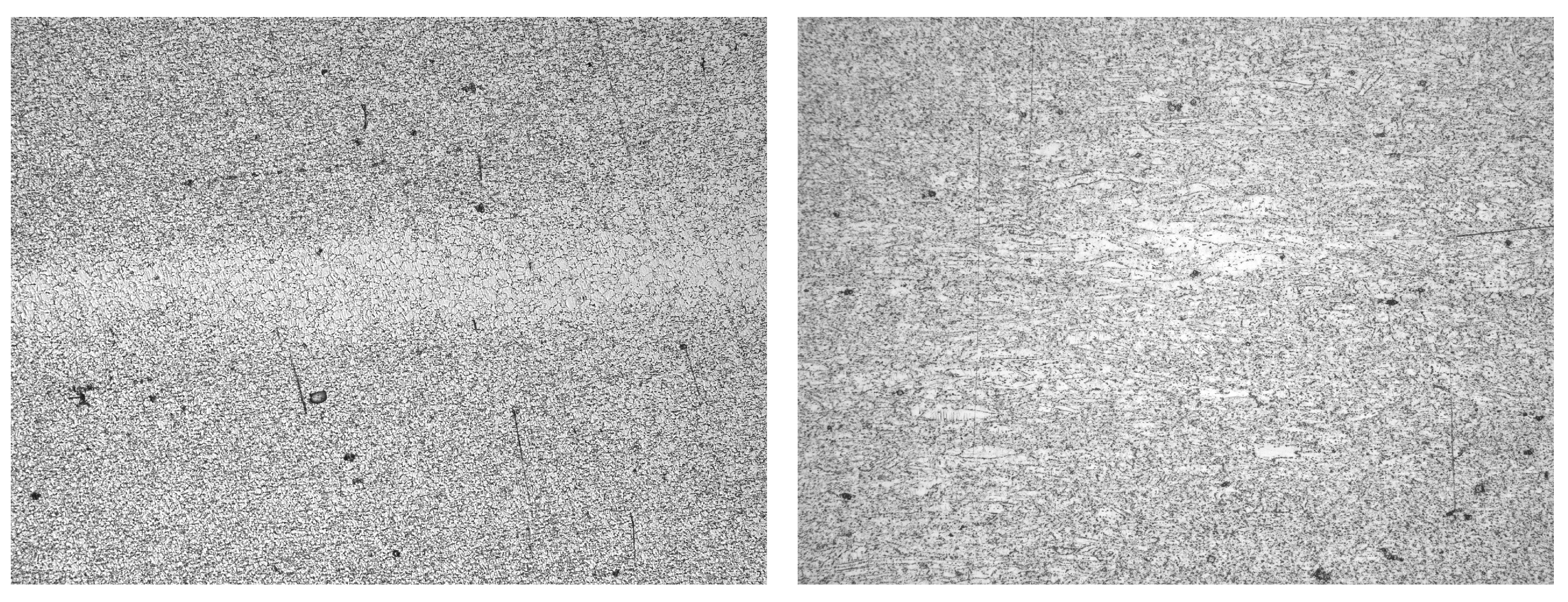
The material employed in this study is Inconel 718, which is a well-known alloy for turbine disk applications. This nickel-superalloy is a popular material in aircraft engine components due to its excellent mechanical properties, high temperature strength and corrosion resistance [42]. The material is typically produced by a double or triple melting process, followed by thermomechanical processing and heat treatments [43,44,45]. Various defects can be attributed to this complex manufacturing process. Distinct examples of those defects are displayed in Figure 1. One of the most prevalent defects is the so-called white spot (WS). Such defects are created if material from the shelf or crown of the melt pool, or from the electrode during the vacuum arc remelting (VAR) process, falls into the melt and is not completely dissolved before reaching the solidification zone. White spots are chemical segregations of the alloying elements, which are typically sharply separated from the surrounding matrix material and contain significantly larger grains than the matrix [46,47]. The formation of white spots is typically accompanied by a reduction in the niobium content, which results in a depletion of the N i 3 N b δ and γ phases. This worsens the properties of the material, because, on the one hand, the precipitation of the δ phase at the grain boundaries is crucial for preventing grain growth during forging. On the other hand, the precipitation of the γ phase, in combination with the γ phase, represents the primary hardening precipitates of this alloy. Therefore, the region affected by the white spot defect exhibits a notable decline in the mechanical properties [48,49,50,51,52]. Additionally, minor inclusions of oxidic or nitridic material may be introduced into the alloy during the melting process [53]. In the event that an inclusion is present within a WS, the resulting defect is referred to as a Dirty White Spot (DWS). In the absence of inclusions, white spots may be designated as Clean White Spots (CWSs). In the event that an inclusion is not related to a WS and contains oxidic or nitridic impurities, it is designated as a non-metallic inclusion (NMI). The final category of defect within the scope of this study is that of light etching regions, which are designated as Light Etch Indications (LEIs). These inclusions resemble WS in appearance and might contain larger grains. However, in contrast to WS, they lack a sharp boundary to the matrix material and exhibit no strong chemical segregation to the matrix structure. Consequently, the depletion of δ and γ precipitates in these defects is less pronounced than in WS. Such defects may be produced during thermomechanical processing if local temperature peaks exceed the delta-solvus point, or they may result from solidification white spots that form due to instabilities in the solidification rate during the melting process [46]. It should be noted that additional types of defects may occur in this alloy. However, the previously mentioned defects are the most prevalent and are included in the dataset used in this study.
To identify material defects in this alloy, several non-destructive evaluation (NDE) techniques, such as ultrasonic testing or fluorescent penetrant inspection, are employed. The objective of this study is to examine the data generated during macro etch testing. The components are subjected to an anodic etching process, wherein microstructural inhomogeneities result in the formation of a contrast-rich indication on the component relative to the surrounding matrix structure. Subsequently, the microstructures of the indications are obtained by replica technique (lacquer imprints) and analyzed under light optical microscopes. Finally, the microstructure of the replica is evaluated by experts and classified as a potential defect if it deviates from the regular microstructure. The differentiation of specific defect types, such as LEI and CWS, can prove challenging even for experts in this field. Accordingly, the definitive classification is determined through a consensus of multiple experts, rather than relying on a single determination. In some instances, the evaluation indicates that an etch indication was present on close to regular microstructure with just minor deviations, resulting in the designation “conform”. Consequently, the etch inspection dataset comprises five distinct outcomes:
  • Conform
  • Light Etch Indication (LEI)
  • Clean White Spot (CWS)
  • Dirty White Spot (DWS)
  • Non-Metallic Inlcusion (NMI)
Figure 1 illustrates the full range of defect classes and the corresponding microstructure for each class. Additional samples are displayed in Appendix A.
At the outset of this project, a database comprising approximately 1000 micrographs of material defects and non-defect indications was assembled from serial metallographic testing. The distribution of data by class is illustrated in Table 1. The distribution does not represent the actual distribution of defects that occur during the testing process. The images of more critical defects were accumulated over an extended period of years to ensure the availability of sufficient examples. As is typical in NDE data, the most severe melting defects (e.g., DWS and NMI) are scarce due to their rare occurrence during the manufacturing of the parts. Consequently, these defect classes significantly restrict the dataset if a balanced class distribution is the objective. Additionally, the number of conform samples is relatively limited due to their status as ’false positives’ of the macro etch process. This class could be easily augmented by producing supplementary replicas of the conform matrix material of the parts.

2.2. Experimental Datasets

In order to evaluate and compare the effect of traditional data augmentation and our synthetic data framework, a balanced subset of the initial data is sampled. The number of samples in this set is limited to 106 images per class, due to the fact that the smallest class of DWS is particularly under-represented. Furthermore, additional reduction in the training data is necessary to create an independent test set. The test set comprises approximately 20% of the balanced data, containing 21 images per class, with the remaining 85 samples per class allocated to the remaining training data. As a result of these necessary reductions in the initial dataset, the number of samples has decreased significantly, highlighting the challenges that must be overcome if balanced datasets are to be used in an NDE deep learning application. The effect of increasing data imbalance is investigated by the generation of several sub-datasets. The number of samples in the conform material class is maintained at 85, while the number of samples in the defect class is reduced in accordance with the designated imbalance ratio of their associated ρ metric, introduced by the authors of [16]:
ρ = m a x i { | C i | } m i n i { | C i | } ,
The metric is defined by the ratio of the largest class C i to the smallest class, defined in Equation (1). The distribution of the data in all datasets is presented in Table 2.
Furthermore, four additional datasets are generated from the four subsampled sets. In these datasets, each defect class is populated with synthetic samples of the class until the initial balanced state of 85 images per class is reached again. Accordingly, the set with a ρ ratio of 20 contains 81 synthetic images per defect class, the set with a ratio of ρ = 2 contains 43, and all sets in between contain the same number of synthetic images per defect class. The total number of samples in all synthetic datasets is 425, which is equivalent to the initial balanced dataset. The comprehensive distribution of data within each dataset is presented in Table 3.
The classification of these defects is a challenging task, particularly when the sample size is limited to less than 100 samples, even in the balanced dataset. Additionally, even human experts in this domain may encounter difficulties in classifying every image without mistakes due to the presence of classes with similar features and the necessity of classifying based on morphology and area fraction of delta phase and grain size, while chemical analysis or complex electron microscopy techniques are not available for an replica-based assessment. In particular, distinguishing between the Conform, LEI, and CWS classes can present a challenge in certain instances. Accordingly, the objective of this study is not to evaluate the initial baseline performance, but rather to examine the discrepancies between the native scores, the classical data augmentation techniques, and our proposed synthetic data approach, particularly in the context of data imbalance.

2.3. Deep Learning Image Classification Framework

In this study, we utilize a CNN as the classifier. The feature extractor comprises established architectures from the public ImageNet benchmark [54]. We add our own classification head due to the lower amount of classes in this use case. The configuration of the classification head remains constant throughout the course of the study, which examines the various architectures of the feature extractor. The results of the model study are presented in Section 3. The classification head is constructed from three fully connected dense layers, comprising 256, 128, and 32 nodes, respectively. A dropout [55] rate of 50% is employed for each layer during the training phase. A rectified linear unit (ReLU) activation function is employed, and each layer is subjected to L1 and L2 regularization with an alpha parameter of 5 · 10 4 and 10 3 , respectively. To ensure the fairness of the evaluation, all non-trainable hyperparameters are kept constant between the different training runs in our experiments. In order to achieve a more rapid convergence, all models are pre-trained with weights derived from ImageNet training. The transfer learning process is divided into two training runs. In the initial training phase, only the classification head, initialized with random weights, is trained. In the subsequent fine-tuning phase, the feature extractor and classification head are trained together, with only 25% of the feature extractor layers unfreezed to preserve the knowledge gained from the ImageNet pre-training. A learning rate of 10 3 is used during the initial training phase, and a learning rate of 10 5 is used during the fine-tuning phase. To further regularize the model and prevent overfitting on this limited dataset, we employ two additional techniques: Focal Loss [14] and Label Smoothing [56]. The Label Smoothing hyperparameter is set to 0.5 , and the γ value of Focal Loss is set to 2. The value of the α parameter for Focal Loss is set to 1 for all balanced sub-datasets, including those that have been artificially balanced with synthetic data. In the case of the imbalanced sets, class weighting is applied on the alpha parameter. Traditional data augmentation techniques, such as rotations and minor adjustments to contrast and brightness, are applied prior to training with exception of the initial model trainings. In order to mitigate the impact of the imbalance, the augmentation strategy employs oversampling, whereby a greater number of augmentations are applied to the minority classes than to the majority class. To reduce the impact of the increasingly small validation set for subsets with high imbalance, the complete training loop is executed within an outer five-fold cross-validation framework. The validation split is stratified by the label class to ensure that high ρ sets retain an equivalent representation of each defect class in the validation set. In succession to the training the models are all validated on the independent test set built from only real samples which are not included in any of the train datasets.

2.4. Round Robin Test

To gain further insight into the key characteristics of the synthetic data, a round robin test was conducted with five experts who are familiar with the material and its defect characteristics. All experts involved have a background in materials science or engineering and possess in-depth knowledge of the material and its associated defects. They work within the manufacturing chain of turbine engine components and serve as members of a dedicated panel responsible for evaluating these defects on a weekly basis. Consequently, these experts have substantial experience and expertise in the classification of such defects.
The test is divided into two parts. The initial objective is to determine the difficulty level of differentiating between real and synthetic samples and to identify the specific features that humans utilize to distinguish the synthetic samples. Moreover, it is essential to ascertain that the synthetic images are not misclassified with greater frequency than their real counterparts within each category. Otherwise, the utility of the synthetic samples would be called into question. In the second split, the quality of the real and synthetic samples is compared by class. This investigation aims to ascertain whether the quality is comparable to that of the real samples and whether some classes are of a lower quality than others. This information is valuable for the improvement of future synthetic data generation.
Fleiss’ Kappa was calculated to quantify the inter-rater agreement among experts during the evaluation of categorical responses in the first test. The metric quantifies the ratio of rater agreement above chance in proportion to the maximum attainable rater agreement [57]:
κ = P ¯ P ¯ e 1 P ¯ e
Hereby the observed agreement P ¯ and the expected agreement P ¯ e are computed from the tests data. For the second test, the standard deviation of the quality scores for the synthetic samples was measured and compared to the standard deviation of the control group. This comparison allows the standard deviation to serve as an indicator of significant differences in expert assessments on one hand, and deviations from the real control samples on the other.

2.5. Multiresolution Stochastic Texture Synthesis Framework

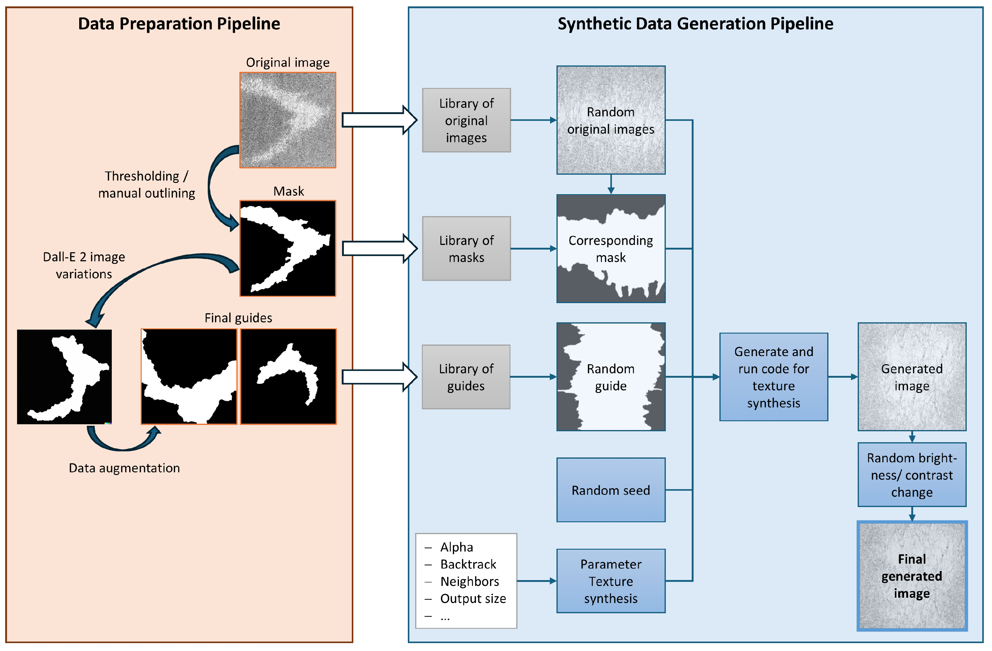
The implementation of the multiresolution stochastic texture synthesis is based on a computer graphics design approach developed by Embark Studios (www.embark-studios.com, accessed on 10 October 2024). The code is available in the Rust programming language and can be downloaded from (https://github.com/embarkstudios/texture-synthesis, accessed on 10 October 2024). The particular methodology employed for the generation of our defect micrographs is designated as “guided synthesis.” This approach permits the consideration of up to three distinct textures. Three input images are required for the generation of a new synthetic example: (1) the original image, (2) a binary mask of the original image indicating the locations of the different textures, and (3) a guide indicating the desired locations for the creation of the different textures in the synthetic image. The masks were generated in one of two ways. In the first instance, the different image textures were manually annotated. In the second instance, a threshold segmentation was employed, with tailored pre- and post-processing, if the quality of the replica image allowed for it. In the case of the LEI and CWS classes, the initial texture is the matrix texture, which represents the regular fine-grained microstructure, while the subsequent texture is the coarse-grained microstructure. In the case of the NMI class, the initial texture is also the matrix texture, while the subsequent texture represents the particles and stringers of the non-metallic inclusions. The masks of these classes are encoded as binary images. The class DWS comprises three distinct textures, and thus is encoded as an RGB image. The initial texture is once again the matrix texture, the second is the coarse-grained microstructure, and the third is the non-metallic inclusion. In order to facilitate the transition between the two textures, a Gaussian blurring with a radius of ten is applied to both the masks and the guides for the LEI class. This is due to the fact that this particular type of defect does not exhibit the pronounced sharpness between the fine-grained and coarse-grained microstructure that is characteristic of the CWS and DWS classes. The synthetic data should be represented by guides that differ from the original dataset in a meaningful way. Therefore the guides should exhibit a distinct visual profile compared to the existing data. Additionally, the resulting shapes should be realistic and not contain any unrealistic features. The generation of the guides was conducted through a two-step process. Initially, the DALL-E 2 (https://openai.com/index/dall-e-2/, accessed on 13 October 2024) image generator from OpenAI was employed to generate variations of the original masks. Only the graphical user interface and the “generate image variations” option were utilized for this study. Variations that appeared metallurgically plausible were manually selected for inclusion. To enable scalability of the approach, the generation of variations could be automated via the application programming interface (API). Furthermore, filters derived from the characteristics of manually selected variations, such as realistic shape and size or in general contour features, could be implemented to ensure that the final selection process remains as objective and efficient as possible. In addition to the DALL-E variations, conventional data augmentation was applied to these images, encompassing a range of transformations such as rotation, flip, translation, zoom, crop, resize, and shear. This process ensures that the resulting guides possess realistic shapes comparable to those of the original defects, while still exhibiting sufficient divergence from the original defect appearance. In order to generate a synthetic image, it is first necessary to randomly select an original image and its corresponding mask. Subsequently, a guide is randomly selected, and a synthetic image is generated based on the three requisite input images. To guarantee the synthesis of disparate images even when the original image and guide remain unchanged, a random seed is integrated to establish the initial point of texture synthesis. The hyperparameters for the texture synthesis were set to their default values, and the output size of the generated image was set to 1024 × 1024 pixels, following an initial parameter study. The default settings were adopted from the values described in the source. To further enhance the variability of the dataset, a random brightness and contrast alteration was implemented to the generated synthetic images. The complete generation framework is visualized in Figure 2. A comparison between some real samples and some synthetic samples generated by this framework is presented in Appendix A.
For each subsample of the dataset, only the images from the training set and their corresponding masks were used to create the guides and subsequently synthesize the new images. The synthetic data generation framework did not leak any data from the larger sets, the test set, or data that was outside the scope of the project. One hundred samples were generated for each class, resulting in a total of 400 samples. Subsequently, the required number of synthetic images was randomly sampled for each class based on the value of the ρ metric in every subset. The content of the rebalanced datasets is presented in Table 3.

3. Results and Discussion

In the initial stage of the process, the objective is to identify the most appropriate model for working with the data in question. Accordingly, a model study is conducted with some of the most prevalent CNN utilized in the ImageNet benchmark. The models were evaluated using five-fold cross-validation on the original balanced dataset, which consisted exclusively of real examples. No data augmentation techniques were employed. The model performance is assessed exclusively based on the cross-validation accuracy, rather than on the test dataset, to prevent any information from the test dataset from influencing the model selection process. The models in the evaluation and their corresponding cross-validation accuracies are listed in Table 4. The DenseNet169 [58] architecture achieved the highest cross-validation accuracy of approximately 0.75 in our study. Accordingly, this model is employed as the feature extraction backbone in the subsequent experiments. The model, trained on the balanced dataset, achieved a test set accuracy of 0.80 and a macro-average F1 score of 0.79 . This represents the baseline performance for our experiments. The values suggest that the problem is challenging due to the visual similarity of some classes and the limited number of samples, even in the balanced case. However, this case serves as an excellent illustration of a real-world non-destructive testing scenario, where achieving a satisfactory level of reliability is often challenging. The class-wise evaluation indicates that the F1 score for the melting defect classes (CWS, DWS, and NMI) is between 0.8 and 0.9 , while the Conform indications and the LEI reach only 0.77 and 0.64 , respectively. This is advantageous in this case because the melting-related defects are known to have a more significant adverse effect on mechanical properties, necessitating a high degree of reliability in their detection.
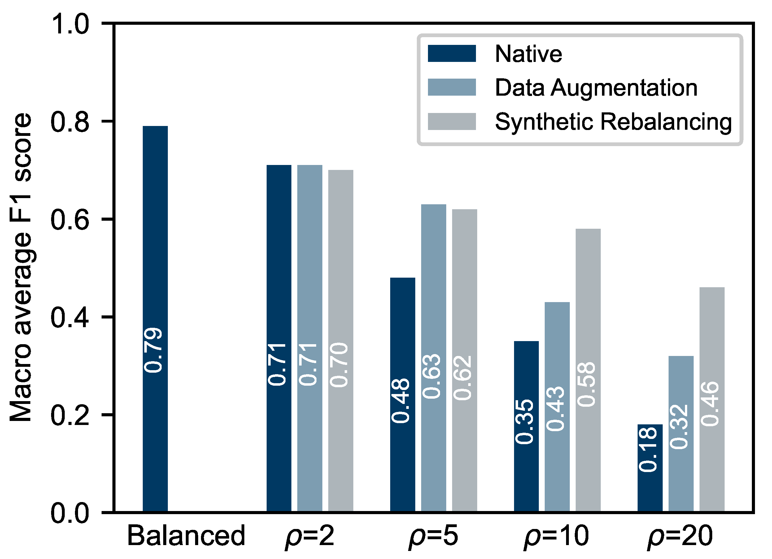
Figure 3 illustrates the comprehensive findings of this investigation. In the initial iteration, the model was trained without the incorporation of synthetic samples or data augmentation, relying solely on the real data from each subset. Subsequently, the performance of each trained model is assessed using the independent test set. As anticipated, the macro-average F1 score on the test set declines with an increase in the ρ ratio. Although the decline from the balanced set to ρ = 2 is relatively modest, the reduction in F1 score is significant in the subsequent step, where it reaches only 0.48 with an imbalanced ratio of ρ = 5 . As anticipated, the score declines further, reaching a minimum of 0.18 for the heavily imbalanced subset with a ratio of ρ = 20 , which has only four training samples per defect. In the following step, the model’s performance is enhanced through the application of classic data augmentation techniques. The model is not reevaluated on the balanced set, as no significant improvement is anticipated and the objective of this study is to enhance the model’s reliability in handling imbalanced data. The results demonstrate no discernible difference with respect to the first imbalanced subset; however, a notable enhancement of approximately 0.1 to 0.15 in the macro-average F1 score is observed for the range of ratios from ρ = 5 to ρ = 20 . In the final iteration, the model is trained on the datasets that have been rebalanced with the synthetic samples, which are described in Table 3. Furthermore, the rebalanced datasets are augmented in accordance with the classic data augmentation technique to enhance the variability in the training data. It should be noted that no oversampling is applied in this case, as the datasets have already been balanced through the incorporation of synthetic data. The synthetic samples were augmented in a manner consistent with that employed for the real data, with the objective of maintaining class balance. In comparison to the runs that solely employed data augmentation, the scores for the first two splits are approximately equivalent. In the case of the split with a ratio of ρ = 2 , it seems that neither classic data augmentation nor synthetic rebalancing can enhance the performance. In the case of the dataset with a ratio of ρ = 5 , both methods yield a higher score than the native approach. These findings suggest that the application of synthetic samples or data augmentation may not result in enhanced model performance in instances where the degree of imbalance is relatively low and an adequate number of real examples are available. However, this remains uncertain due to the low difference in F1 score, which may be a special case for this data and model combination. Further research is required to substantiate this conclusion. In cases of high imbalance, with ratios of ρ = 10 and ρ = 20 , the F1 score demonstrates a notable enhancement in comparison to the approach involving solely conventional data augmentation. The model trained on the subset exhibiting the greatest imbalance can still achieve an F1 score of 0.46 , which is approximately equivalent to the level achieved by the native model for ρ = 5 . In general, the synthetic rebalancing method demonstrates superior performance compared to classic data augmentation techniques, particularly in scenarios with higher imbalance ratios. For moderate imbalance levels, the two approaches exhibit comparable outcomes. The results lend support to the hypothesis that the extent of artificial variation introduced into the dataset by data augmentation is limited. In particular, the variance achievable through data augmentation is contingent upon the quantity of real data present within the dataset. Therefore, the datasets with low imbalance, which still contain sufficient real samples, are on a similar level to the synthetic rebalanced datasets. However, the splits at ρ = 10 and above appear to lack sufficient real samples to achieve sufficient variance through data augmentation. It is currently unclear whether the limit at which this effect becomes significant is always at this ρ -ratio or if this depends on the dataset and the model architecture. Further research in this area would be beneficial.
The class-wise performance metrics are presented in Appendix B. Based on the results for ρ = 10 and ρ = 20 , no clear trend emerges regarding which classes benefit most from the introduction of synthetic data compared to data augmentation. The effect appears to depend on the imbalance ratio and on areas where the model previously struggled without synthetic data. For ρ = 10 , there is a significant improvement in the F1 scores for the classes Conform, LEI, CWS, and NMI, while DWS remains at the same level. For ρ = 20 , the F1 score for Conform is comparable to the previous setting, whereas LEI, DWS, and NMI show significant improvements, and CWS exhibits moderate improvement.
One potential avenue for enhancing the model’s performance is to apply data augmentation exclusively to the real dataset and utilize a greater number of synthetic samples to compensate for the examples generated through data augmentation. This approach could prove beneficial for model training, as the additional synthetic samples may offer more useful variations for the model than the augmented synthetic images used in our study. However, a potential drawback is the necessity for significantly more synthetic samples to be generated and stored in advance, whereas data augmentation can be applied online and temporarily stored during the training process. Given the constraints in time and computational resources, this approach was not explored in this study.
To further investigate the quality of the synthetic samples, two round robin tests were conducted. In the initial iteration, 30 images were randomly selected from each defect class, with 15 images being authentic and 15 being synthetic. Five experts in the field of material analysis are tasked with rating each sample as either real or synthetic and providing a brief rationale for their decision. Additionally, the experts are requested to provide their classification of the sample, which is initially unknown to them. The results of this test can be used to identify the features that make the synthetic samples recognizable by human perception. By comparing the human defect classification with the classification of the real and synthetic samples, it can be determined whether the classification is more accurate for one or the other, or if the accuracy is equal. The evaluation of the aforementioned features, which the experts used to determine whether a sample was synthetic, has led to the identification of the following main features:
  • Features of the inclusions particles such as unnatural shapes or unrealistic patterns.
  • Periodic artificial structures, i.e., patterns in the matrix structure or stripes in the inclusions.
  • Unnatural shape of the defect area.
  • General artifacts.
  • Grain boundaries missing or too weak.
  • Boundary between matrix and defect area too sharp.
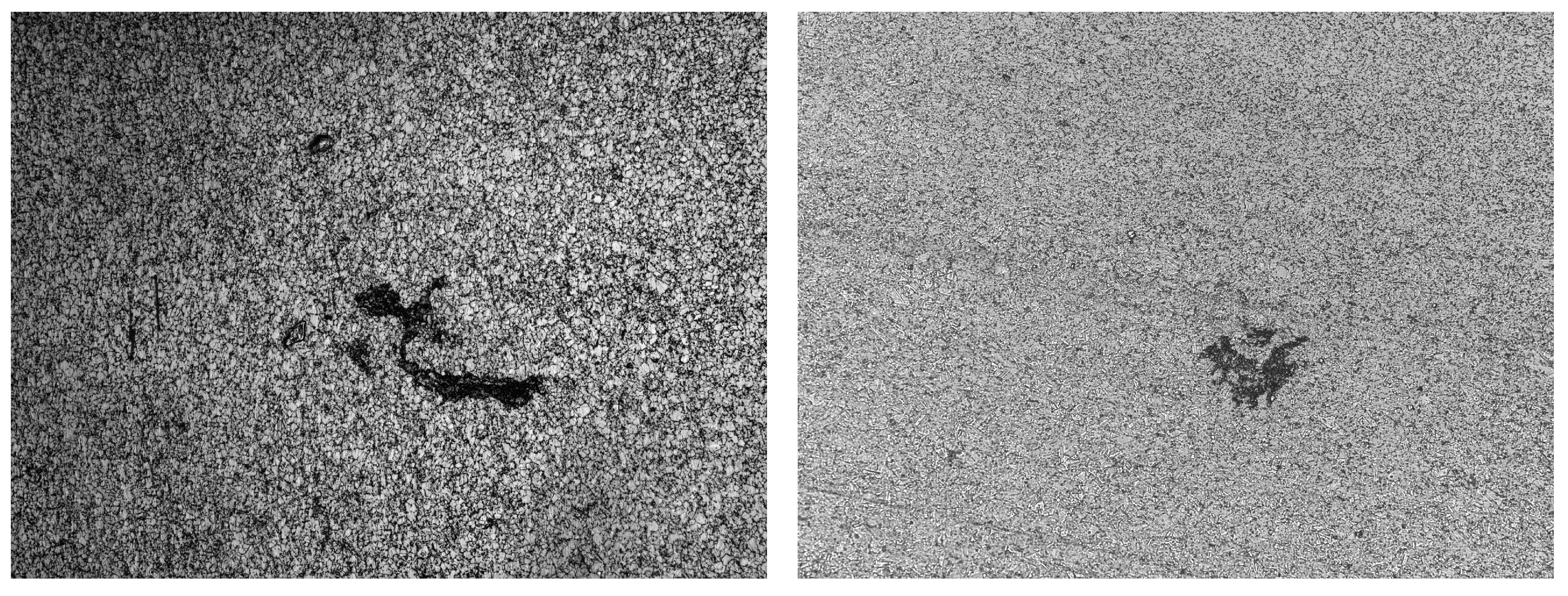
These six features comprised the top 75%-percentile of the distribution of named features. Only those features that were associated with a true positive identification of a synthetic sample were counted. The features identified real samples that were incorrectly classified as synthetic are not included in the subsequent analysis. Two of these features are depicted in Figure 4.
No clear description of known artifacts associated with the multiresolution stochastic texture synthesis algorithm could be found in the literature. However, some features can be inferred from the nature of the algorithm itself. Periodic structures, such as patterns in the matrix, are generated because non-parametric texture synthesis relies on copying and reusing certain patterns from the provided example image. Consequently, texture patches may sometimes be reused too frequently or placed in locations where they appear unnatural. Over time, techniques have been introduced to mitigate issues such as “garbage-growing,” which refers to the copying of irregularly shaped patches. Nevertheless, this behavior has not been completely eliminated and remains a weakness of the synthesis algorithm. Unnatural shapes or patterns within inclusions likely originate from their inherently irregular characteristics, which are more difficult to reproduce as textures compared to the more regular coarse-grain or matrix structures. Additionally, unnatural defect shapes may occur under certain conditions due to local optimization at each scale and the absence of global constraints on boundary geometry. This limitation could potentially be addressed by incorporating additional filters or constraints on boundaries at the global image scale.
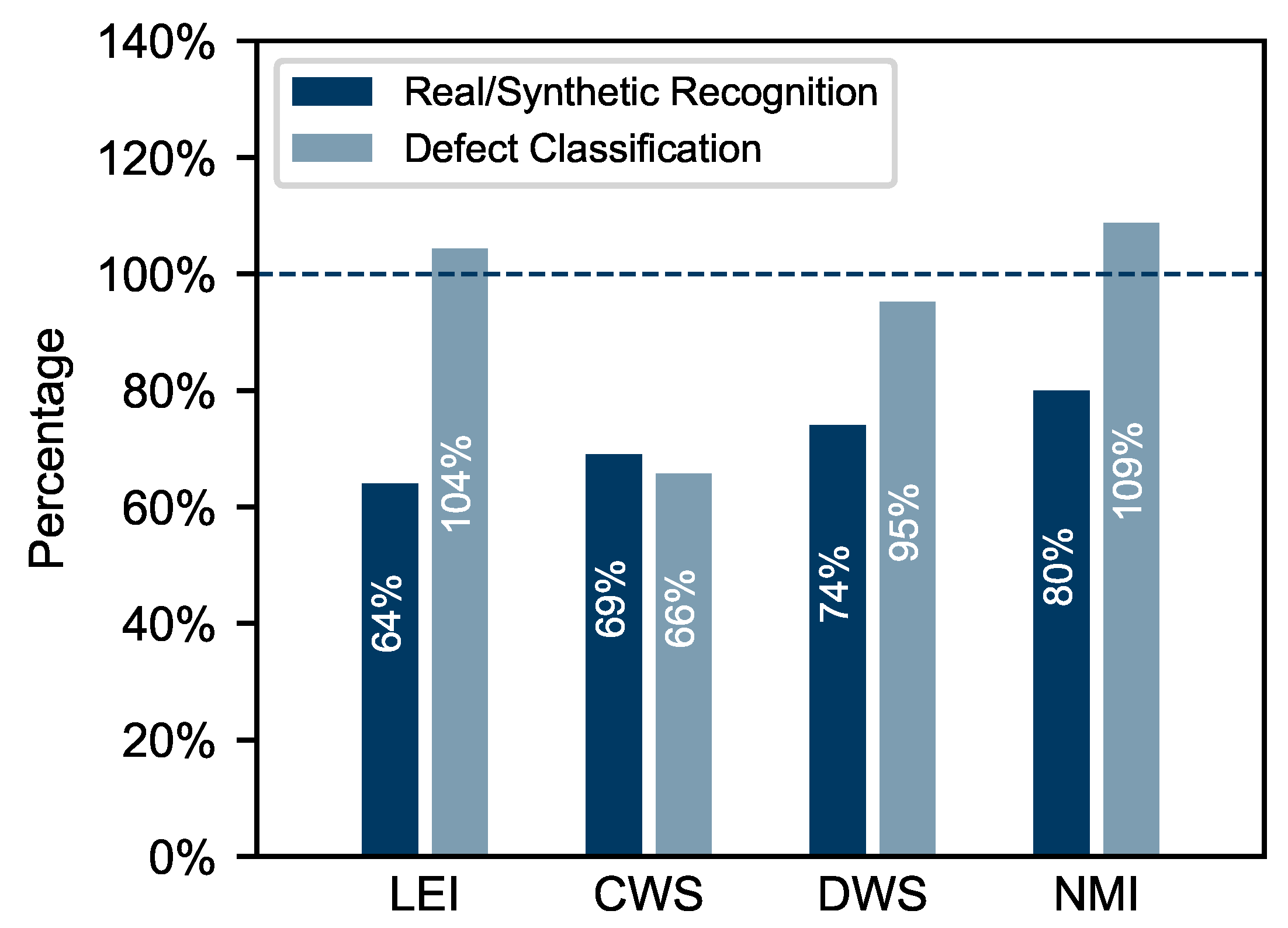
The remaining results of this test are presented in Figure 5. The Fleiss’ Kappa values for the first part of the test are presented in Table 5. For the first question of the test, the Kappa values indicate moderate agreement among experts, suggesting that distinguishing between synthetic and real samples is challenging due to the overall high quality of the samples. Nevertheless, the experts agree more often than expected by chance, demonstrating that meaningful conclusions can be drawn from the results. For the second test, the Kappa value reflects substantial agreement among experts. Their rating of defect classes shows stronger consistency, which is plausible given their significant expertise in evaluating these defects. Therefore, the classification results provide a reliable basis for drawing meaningful conclusions.
As illustrated in Figure 5, the experts demonstrated a high degree of accuracy in identifying whether a sample was real or synthetic. The lowest percentage is observed for the LEI class, while the highest is observed for the NMIs. This is consistent with the identified features, which were frequently concentrated on the characteristics of the inclusions, which are exclusive to the DWS and NMI samples and absent in the LEI and CWS samples. The experts encountered the greatest difficulty in identifying features that would distinguish synthetic samples within the LEI class. The results demonstrate that our synthesis framework is capable of generating pure coarse-grain defects with sufficient fidelity. However, there is room for improvement in generating defects that contain irregular structures, such as particles and inclusions. The columns in Figure 5 designated as “Defect Classification” represent the percentage of correctly classified synthetic samples in relation to the real samples. Since the experts’ classification in this case is based on individual decisions rather than the regular majority vote, there is a possibility of discrepancies between the ground truth class and the individual classification. Consequently, a value of 100 % signifies that the synthetic samples of this defect class were classified correctly at the same frequency as the real samples of this class. Conversely, a value exceeding 100 % indicates that the classification accuracy of the synthetic samples was superior to that of the real samples on average. Excluding the CWS class, the Defect Classification is approximately 100 % for all remaining classes. This indicates that our synthetic data is capable of replicating the distinctive features that define these classes in human perception. It seems reasonable to conclude that the significant features used by the AI model to identify these classes have also been incorporated. The CWS class may be a unique case, as the differentiation between the LEI and CWS classes can be challenging even for human experts. It is thus conceivable that our data generation model was unable to produce samples in which the distinction between these classes was sufficiently pronounced. Nevertheless, an examination of the class-wise F1 score results does not suggest that the AI model exhibits a general deficit in performance with regard to this class over the synthetic data subsets. One potential explanation is that the model is sensitive to different features than human experts, which are adequately represented by the framework.
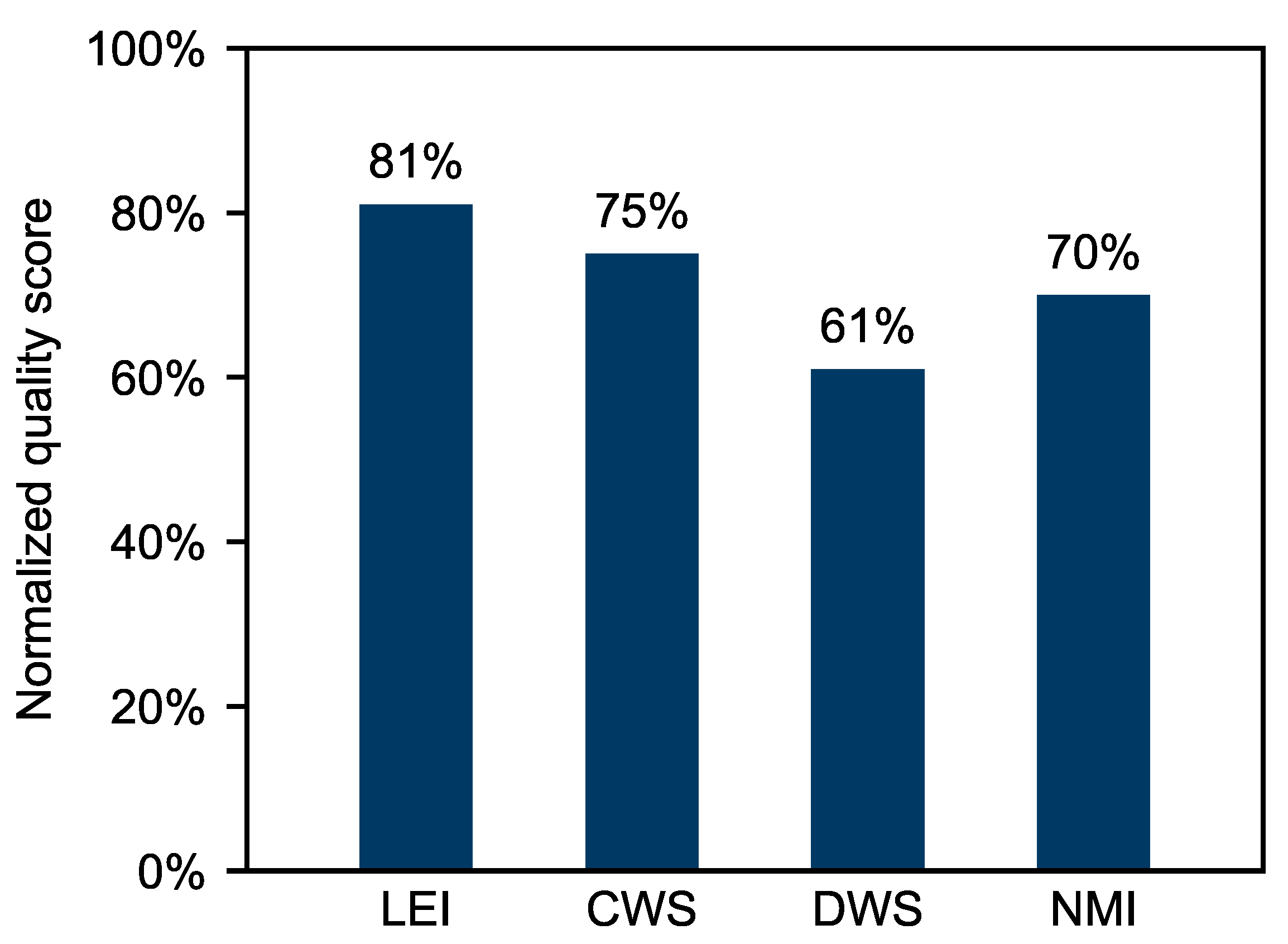
In the second variant of the round robin test, a total of 25 images are selected at random from each defect class. The images are stored in a sorted format to ensure that the experts are aware of the ground truth defect class associated with each sample. The images in question contain 20 synthetic defects and 5 real defects. However, the experts have been informed that all samples are synthetic. In this iteration of the experiment, the objective is to assign a rating to each sample on a scale of one to five, with five indicating a high degree of realism and one indicating a clear synthetic origin. The reason for the inclusion of the five real samples per class is that they serve as a control group. The rating of the real samples enables the normalization of the subjective judgments of the experts regarding the synthetic samples. The standard deviations of the quality scores by class are shown in Table 6. Overall, the standard deviations in each class are low, approximately 1 or below, indicating that the experts rated the quality of the samples quite consistently, with good agreement. The maximum difference between the standard deviation of synthetic and real samples is 0.2, which is therefore highly comparable. This suggests that the variability in quality scores for the synthetic samples is similar to that of the real control samples, allowing meaningful conclusions to be drawn from these results. The results of this test are presented in Figure 6. The LEI class samples were, on average, rated the highest in quality, while the DWS class was rated the lowest. The favorable outcome for the LEI class is consistent with the experts’ greater challenge in discerning the synthetic samples during the initial assessment. The DWS class was primarily affected by the inferior quality of the inclusions in certain samples, as evidenced by the primary synthetic features enumerated in the initial test. The quality of all classes is, on the whole, slightly worse than that of the real samples. But considering the synthetic origin of the samples, reaching quality scores of over 70 % for three of four classes is considered a success. However, this test again confirms the necessity for improvement in the generation of classes containing inclusions for future studies.
The results of the round robin test indicate that it may be beneficial to investigate the potential benefits of removing negatively rated synthetic data in order to enhance the overall classification performance. To achieve this, the round robin results, which due to time constraints of the experts could only be performed on a subset of the synthetic data, must first be transformed into a suitable image metric, which is then used to filter out all inadequate synthetic images. However, simple image metrics, e.g., non-reference image metrics such as Brisque [66] or Piqe [67], did not correlate with the expert judgments, i.e., the quality scores assigned to the synthetic images. In the end, a combination of Brisque, Piqe, and a bag of visual word features [68] was chosen. A quality score of 65% was established as the threshold for sufficient quality. Subsequently, a classification model was constructed and trained using the aforementioned features on the 80 images from the second variant of the round robin test. The model was consequently employed for the classification of the full set of synthetic images from the ρ = 2 data split, with the objective of determining their quality. As a result, 142 of the 400 synthetic images were excluded, representing approximately 35% of the total number of synthetic samples. This result appears to be consistent with the expert judgments.
Subsequently, the filtering process yielded a new ρ = 2 dataset comprising solely synthetic samples of high quality, which were then subjected to retraining of the model. The model achieved a test set F1 score of 0.75 on this new iteration. As evidenced by the results, the model exhibited an increase of 0.05 in its F1 score, compared to the unfiltered dataset, thereby attaining the highest performance in this split, with a mere 0.04 point separating it from the native performance. This illustrates that the filtering of the synthetic samples with the model calibrated on the basis of expert judgment could enhance its performance. Although it initially appeared that the score could not be improved in the case of the ρ = 2 dataset, it has now been demonstrated that synthetic rebalancing is indeed capable of doing so. However, it seems likely that the model is sensitive to the synthetic samples used. In conclusion, the synthetic rebalancing method has been shown to outperform classic data augmentation even in this low imbalance case. By applying an automated filtering process in the generation pipeline, it is probable that the quality of future datasets could be enhanced.
As it appears that inadequate synthetic samples can compromise the maximally achievable classification performance, the synthetic data generation pipeline could be improved for future work to avoid the time-consuming round robin test that was used to filter out the inadequate samples in this work. Due to the stochastic nature of the texture synthesis, options to intervene are rather limited. This makes it difficult to counteract some of the synthetic image features, such as periodic matrix structures, identified by the experts. However, unnatural shapes, which were frequently mentioned as features associated with lower quality scores, could be improved in future work by defining values for typical shapes. The masks of all the original images could be used to determine the typical shapes, and targets containing unnatural shapes could be filtered out before being used in the synthetic data generation. Greater blurring of the targets to make the boundaries between matrix and defect appear less sharp could also be implemented.
A final question of interest is whether the most effective model, trained on synthetic data, could be deployed in a real-world application. Therefore, an analysis of the class-wise F1 score is conducted for the best-performing model, with the exception of the model trained on the initial balanced set. The model in question was trained on the ρ = 2 split, which included the synthetic samples that had been filtered. As illustrated in Table 7, the class-wise score reveals a notable disparity in performance between the LEI class and the remaining ones. This discrepancy is likely attributable to the presence of similar features among the conform, LEI, and CWS classes, which primarily differentiate themselves based on their grain size and the sharpness of the boundaries between the matrix structure and the defect area. Consequently, the model encounters difficulties in identifying the boundaries between these three classes. Fine-tuning the model to distinguish between the conform structure and the three critical melting defects may result in an overall improvement in performance. Such a model may be suitable for implementation in a “human in the loop” framework, whereby the model pre-selects critical defects of the CWS, DWS, or NMI class, and a human expert subsequently reviews the images. In this approach, the metallographer uploads microstructure images of the part under investigation into the AI system. The AI then classifies the defects and highlights any critical melting defects so they can be prioritized for analysis. If a critical defect is confirmed by experts, the part is typically scrapped. By ordering defects according to model predictions, experts would likely examine the most critical defects first and could skip remaining indications on a part where a critical defect has already been identified. This would allow the expensive time of experts to be used more effectively. An additional possibility to increase efficiency is to scrap parts containing critical defects immediately after model inference, without expert review, leveraging the high accuracy of the model for critical defects. This approach would reduce throughput time and increase overall production capacity. Whether this is economically viable depends on the production cost of the parts at this stage, the cost of expert time, and the model’s accuracy. This strategy could be a significant production booster for manufacturing relatively inexpensive parts in large quantities that are prone to material defects. Finally, efficiency could be further improved by skipping expert review for parts where the model classifies all indications as conform. While this is not a realistic approach for the highly safety-critical aerospace parts considered in this work, it could be feasible for parts produced in high volumes that do not directly affect safety. For less expensive parts that do not undergo intensive quality control procedures, such an NDT methodology could provide a practical option for implementing quality control at all, improving product quality while keeping production costs relatively low.

4. Conclusions

This study evaluated the efficacy of rebalancing imbalanced datasets through the incorporation of synthetic data, with a case study on material defect classification in Inconel 718 turbine disks. By comparing the native performance of the image classification model with the use of data augmentation and the training with synthetic data, it was demonstrated that the proposed synthetic rebalancing approach achieves a markedly elevated test set F1 score in high imbalance datasets. The multiresolution stochastic texture synthesis approach has the advantage of requiring only a limited number of images, which is a significant benefit when compared to data-driven approaches that necessitate the initial training of a generation model with hundreds or thousands of samples. These models are usually not applicable to the domain of non-destructive evaluation, as they have limited amounts of training data. The quality of the synthetic images was validated through expert round robin tests with both real and synthetic images. By translating expert judgments into image quality scores to filter out synthetic images with insufficient quality from the dataset with the imbalance ratio ρ = 2 , the F1 score was enhanced to a level approaching that of the full-sized, balanced reference dataset. This indicates that the automated filtering of synthetic samples may be advantageous for the generation process and classification outcomes. In conclusion, the results demonstrate that synthetic rebalancing through multiresolution stochastic texture synthesis is an effective method for improving performance in datasets with inherent imbalance.
Future research should focus on the reduction in the artificial features identified by experts in the dataset, with the objective of improving the generation of the defect classes containing inclusions. Furthermore, the integration of autonomous filtering of low-quality synthetic samples into the generation framework would result in an overall improvement in the quality of the synthetic data. The implementation of a model or image quality metric that does not necessitate calibration based on human experts would be advantageous from an engineering standpoint. In addition, an assessment of the generation framework in relation to further use cases based on image data with periodic textures, such as macroscopic surface quality assessment, could represent a potential focal point for future research. To adapt the proposed synthesis framework to other applications and to tailor the synthesis model to arbitrary surface defects in different materials or components, the process of collecting a library of masks, images, and target masks must be replicated. The only strict requirements are that both the defect area and the underlying background can be segmented, that the defect and surrounding background exhibit texture-like characteristics, meaning they are composed of similar recurring structures, and that no more than three segmentated phases are used. Finally, the framework’s hyperparameters must be adjusted to the new dataset to ensure that the quality of the generated samples is sufficient.

Author Contributions

Conceptualization: Y.N.S. and M.M.; Methodology: Y.N.S. and M.M.; Software: Y.N.S. and M.M.; Validation: Y.N.S. and M.M.; Investigation: Y.N.S.; Resources: Y.N.S.; Data Curation: Y.N.S. and M.M.; Writing—Original Draft: Y.N.S. and M.M.; Writing—Review and Editing: Y.N.S., M.M., and F.M.; Visualization: Y.N.S. and M.M.; Supervision: F.M. All authors have read and agreed to the published version of the manuscript.

Funding

This research received no external funding.

Data Availability Statement

The datasets presented in this article are not readily available because the data are part of an ongoing study. Requests to access the datasets should be directed to the corresponding author.

Conflicts of Interest

Author Yann Niklas Schöbel was employed by the company MTU Aero Engines AG. The remaining authors declare that the research was conducted in the absence of any commercial or financial relationships that could be construed as a potential conflict of interest.

Appendix A. Image Selection

Appendix A.1. Conform

Figure A1. Real conform examples.
Metals 15 01172 g0a1

Appendix A.2. LEI

Figure A2. Real LEI examples.
Metals 15 01172 g0a2
Figure A3. Synthetic LEI examples.
Metals 15 01172 g0a3

Appendix A.3. CWS

Figure A4. Real CWS examples.
Metals 15 01172 g0a4
Figure A5. Synthetic CWS examples.
Metals 15 01172 g0a5

Appendix A.4. DWS

Figure A6. Real DWS examples.
Metals 15 01172 g0a6
Figure A7. Synthetic DWS examples.
Metals 15 01172 g0a7

Appendix A.5. NMI

Figure A8. Real NMI examples.
Metals 15 01172 g0a8
Figure A9. Synthetic NMI examples.
Metals 15 01172 g0a9

Appendix B. Class-Wise Metrics

Table A1. Class-wise metrics of the native data.
ρ ClassPrecisionRecallF1 Score
1Conform0.830.710.77
LEI0.610.670.64
CWS0.890.810.85
DWS0.810.810.81
NMI0.830.950.89
2Conform0.700.750.72
LEI0.700.750.72
CWS0.810.620.70
DWS0.850.520.65
NMI0.670.950.78
5Conform0.410.860.55
LEI0.000.000.00
CWS0.580.710.64
DWS0.750.430.55
NMI0.650.710.68
10Conform0.300.950.45
LEI0.000.000.00
CWS0.480.480.48
DWS0.620.240.34
NMI0.780.330.47
20Conform0.261.000.41
LEI0.200.050.08
CWS0.000.000.00
DWS0.420.380.40
NMI0.000.000.00
Table A2. Class-wise metrics of the data augmentation runs.
ρ ClassPrecisionRecallF1 Score
2Conform0.780.670.72
LEI0.560.480.51
CWS0.620.710.67
DWS0.760.900.83
NMI0.850.810.83
5Conform0.530.810.64
LEI0.730.520.61
CWS0.670.480.56
DWS0.590.620.60
NMI0.710.710.71
10Conform0.330.900.48
LEI0.500.140.22
CWS0.500.330.40
DWS0.620.380.47
NMI0.710.480.57
20Conform0.321.000.48
LEI0.500.050.09
CWS0.560.430.49
DWS0.400.100.15
NMI0.440.330.38
Table A3. Class-wise metrics of the synthetic rebalanced data.
ρ ClassPrecisionRecallF1 Score
2Conform0.730.900.81
LEI0.570.380.46
CWS0.740.670.70
DWS0.750.710.73
NMI0.730.900.81
5Conform0.580.680.63
LEI0.520.670.58
CWS0.670.670.67
DWS0.690.430.53
NMI0.650.620.63
10Conform0.531.000.69
LEI0.670.290.40
CWS0.620.620.62
DWS0.620.380.47
NMI0.680.710.70
20Conform0.340.710.46
LEI0.440.190.27
CWS0.600.570.59
DWS0.560.240.33
NMI0.610.670.64

References

  1. Taheri, H.; Gonzalez Bocanegra, M.; Taheri, M. Artificial Intelligence, Machine Learning and Smart Technologies for Nondestructive Evaluation. Sensors 2022, 22, 4055. [Google Scholar] [CrossRef]
  2. Sun, H.; Ramuhalli, P.; Jacob, R.E. Machine learning for ultrasonic nondestructive examination of welding defects: A systematic review. Ultrasonics 2023, 127, 106854. [Google Scholar] [CrossRef] [PubMed]
  3. Mazzetto, M.; Teixeira, M.; Rodrigues, E.O.; Casanova, D. Deep learning models for visual inspection on Automotive Assembling Line. Int. J. Adv. Eng. Res. Sci. 2020, 7, 473–494. [Google Scholar] [CrossRef]
  4. Voronin, V.; Sizyakin, R.; Zhdanova, M.; Semenishchev, E.; Bezuglov, D.; Zelemskii, A. Automated visual inspection of fabric image using deep learning approach for defect detection. In Proceedings of the Automated Visual Inspection and Machine Vision IV, Online, 21–25 June 2021; Beyerer, J., Heizmann, M., Eds.; International Society for Optics and Photonics; SPIE: Bellingham, WA, USA, 2021; Volume 11787. [Google Scholar] [CrossRef]
  5. Yang, H.; Wang, Y.; Hu, J.; He, J.; Yao, Z.; Bi, Q. Deep Learning and Machine Vision-Based Inspection of Rail Surface Defects. IEEE Trans. Instrum. Meas. 2022, 71, 5005714. [Google Scholar] [CrossRef]
  6. Azimi, S.M.; Britz, D.; Engstler, M.; Fritz, M.; Mücklich, F. Advanced Steel Microstructural Classification by Deep Learning Methods. Sci. Rep. 2018, 8, 2128. [Google Scholar] [CrossRef]
  7. Durmaz, A.R.; Potu, S.T.; Romich, D.; Möller, J.J.; Nützel, R. Microstructure quality control of steels using deep learning. Front. Mater. 2023, 10, 1222456. [Google Scholar] [CrossRef]
  8. Alrfou, K.; Zhao, T.; Kordijazi, A. Deep Learning Methods for Microstructural Image Analysis: The State-of-the-Art and Future Perspectives. Integr. Mater. Manuf. Innov. 2024, 13, 703–731. [Google Scholar] [CrossRef]
  9. Azqadan, E.; Arami, A.; Jahed, H. From microstructure to mechanical properties: Image-based machine learning prediction for AZ80 magnesium alloy. J. Magnes. Alloy. 2025, 13, 4231–4244. [Google Scholar] [CrossRef]
  10. Ly, C.; Frazier, W.; Olsen, A.; Schwerdt, I.; McDonald, L.W.; Hagen, A. Improving microstructures segmentation via pretraining with synthetic data. Comput. Mater. Sci. 2025, 249, 113639. [Google Scholar] [CrossRef]
  11. Na, J.; Kim, S.J.; Kim, H.; Kang, S.H.; Lee, S. A unified microstructure segmentation approach via human-in-the-loop machine learning. Acta Mater. 2023, 255, 119086. [Google Scholar] [CrossRef]
  12. Nikolic, F.; Stajduhar, I.; Canadija, M. Casting Defects Detection in Aluminum Alloys Using Deep Learning: A Classification Approach. Int. J. Met. 2023, 17, 386–398. [Google Scholar] [CrossRef]
  13. Leevy, J.L.; Khoshgoftaar, T.M.; Bauder, R.A.; Seliya, N. A survey on addressing high-class imbalance in big data. J. Big Data 2018, 5, 42. [Google Scholar] [CrossRef]
  14. Lin, T.Y.; Goyal, P.; Girshick, R.B.; He, K.; Dollár, P. Focal Loss for Dense Object Detection. IEEE Trans. Pattern Anal. Mach. Intell. 2017, 42, 318–327. [Google Scholar] [CrossRef]
  15. Graczyk, M.; Lasota, T.; Trawiński, B.; Trawiński, K. Comparison of bagging, boosting and stacking ensembles applied to real estate appraisal. In Proceedings of the Intelligent Information and Database Systems: Second International Conference, ACIIDS, Hue City, Vietnam, 24–26 March 2010; Proceedings, Part II 2. Springer: Berlin/Heidelberg, Germany, 2010; pp. 340–350. [Google Scholar] [CrossRef]
  16. Buda, M.; Maki, A.; Mazurowski, M.A. A systematic study of the class imbalance problem in convolutional neural networks. Neural Netw. Off. J. Int. Neural Netw. Soc. 2018, 106, 249–259. [Google Scholar] [CrossRef]
  17. Guo, H.; Li, Y.; Shang, J.; Gu, M.; Huang, Y.; Gong, B. Learning from class-imbalanced data: Review of methods and applications. Expert Syst. Appl. 2017, 73, 220–239. [Google Scholar] [CrossRef]
  18. Hasib, K.M.; Iqbal, M.S.; Shah, F.M.; Al Mahmud, J.; Popel, M.H.; Showrov, M.I.H.; Ahmed, S.; Rahman, O. A Survey of Methods for Managing the Classification and Solution of Data Imbalance Problem. J. Comput. Sci. 2020, 16, 1546–1557. [Google Scholar] [CrossRef]
  19. Mo, N.; Yan, L. Improved Faster RCNN Based on Feature Amplification and Oversampling Data Augmentation for Oriented Vehicle Detection in Aerial Images. Remote Sens. 2020, 12, 2558. [Google Scholar] [CrossRef]
  20. Shorten, C.; Khoshgoftaar, T.M. A survey on Image Data Augmentation for Deep Learning. J. Big Data 2019, 6, 60. [Google Scholar] [CrossRef]
  21. Langenkämper, D.; van Kevelaer, R.; Nattkemper, T.W. Strategies for Tackling the Class Imbalance Problem in Marine Image Classification. In Proceedings of the Pattern Recognition and Information Forensics, Beijing, China, 20–24 August 2018; Zhang, Z., Suter, D., Tian, Y., Branzan Albu, A., Sidère, N., Jair Escalante, H., Eds.; Springer: Cham, Switzerland, 2019; pp. 26–36. [Google Scholar] [CrossRef]
  22. Batool, U.; Shapiai, M.I.; Ismail, N.; Fauzi, H.; Salleh, S. Oversampling Based on Data Augmentation in Convolutional Neural Network for SiliconWafer Defect Classification. In Volume 327: Knowledge Innovation Through Intelligent Software Methodologies, Tools and Techniques; Frontiers in Artificial Intelligence and Applications; IOS Press: Amsterdam, The Netherlands, 2020; pp. 3–12. [Google Scholar] [CrossRef]
  23. Matsuoka, D. Classification of imbalanced cloud image data using deep neural networks: Performance improvement through a data science competition. Prog. Earth Planet. Sci. 2021, 8, 68. [Google Scholar] [CrossRef]
  24. Saini, M.; Susan, S. Data Augmentation of Minority Class with Transfer Learning for Classification of Imbalanced Breast Cancer Dataset Using Inception-V3. In Proceedings of the Pattern Recognition and Image Analysis, Madrid, Spain, 1–4 July 2019; Morales, A., Fierrez, J., Sánchez, J.S., Ribeiro, B., Eds.; Springer: Cham, Switzerland, 2019; pp. 409–420. [Google Scholar] [CrossRef]
  25. Goodfellow, I.J.; Pouget-Abadie, J.; Mirza, M.; Xu, B.; Warde-Farley, D.; Ozair, S.; Courville, A.; Bengio, Y. Generative adversarial nets. In Proceedings of the 27th International Conference on Neural Information Processing Systems—Volume 2, Cambridge, MA, USA, NIPS’14, Montreal, QC, Canada, 8–13 December 2014; pp. 2672–2680. Available online: https://proceedings.neurips.cc/paper_files/paper/2014/file/f033ed80deb0234979a61f95710dbe25-Paper.pdf (accessed on 13 October 2024).
  26. Bowles, C.; Chen, L.; Guerrero, R.; Bentley, P.; Gunn, R.N.; Hammers, A.; Dickie, D.A.; Hernández, M.V.; Wardlaw, J.M.; Rueckert, D. GAN Augmentation: Augmenting Training Data using Generative Adversarial Networks. arXiv 2018, arXiv:1810.10863. [Google Scholar] [CrossRef]
  27. Tanaka, F.; de Castro Aranha, C. Data Augmentation Using GANs. arXiv 2019, arXiv:1904.09135. [Google Scholar] [CrossRef]
  28. Frid-Adar, M.; Klang, E.; Amitai, M.; Goldberger, J.; Greenspan, H. Synthetic data augmentation using GAN for improved liver lesion classification. In Proceedings of the 2018 IEEE 15th International Symposium on Biomedical Imaging (ISBI 2018), Washington, DC, USA, 4–7 April 2018; pp. 289–293. [Google Scholar] [CrossRef]
  29. Khan, A.R.; Khan, S.; Harouni, M.; Abbasi, R.; Iqbal, S.; Mehmood, Z. Brain tumor segmentation using K-means clustering and deep learning with synthetic data augmentation for classification. Microsc. Res. Tech. 2021, 84, 1389–1399. [Google Scholar] [CrossRef] [PubMed]
  30. Kukreja, V.; Kumar, D.; Kaur, A.; Geetanjali; Sakshi. GAN-based synthetic data augmentation for increased CNN performance in Vehicle Number Plate Recognition. In Proceedings of the 2020 4th International Conference on Electronics, Communication and Aerospace Technology (ICECA), Coimbatore, India, 5–7 November 2020; pp. 1190–1195. [Google Scholar] [CrossRef]
  31. Chun, S.; Roy, S.; Nguyen, Y.T.; Choi, J.B.; Udaykumar, H.S.; Baek, S.S. Deep learning for synthetic microstructure generation in a materials-by-design framework for heterogeneous energetic materials. Sci. Rep. 2020, 10, 13307. [Google Scholar] [CrossRef] [PubMed]
  32. Fokina, D.; Muravleva, E.; Ovchinnikov, G.; Oseledets, I. Microstructure synthesis using style-based generative adversarial networks. Phys. Rev. E 2020, 101, 043308. [Google Scholar] [CrossRef]
  33. Lee, J.W.; Goo, N.H.; Park, W.B.; Pyo, M.; Sohn, K.S. Virtual microstructure design for steels using generative adversarial networks. Eng. Rep. 2021, 3, e12274. [Google Scholar] [CrossRef]
  34. Lambard, G.; Yamazaki, K.; Demura, M. Generation of highly realistic microstructural images of alloys from limited data with a style-based generative adversarial network. Sci. Rep. 2023, 13, 566. [Google Scholar] [CrossRef]
  35. Dahmen, T.; Trampert, P.; Boughorbel, F.; Sprenger, J.; Klusch, M.; Fischer, K.; Kübel, C.; Slusallek, P. Digital reality: A model-based approach to supervised learning from synthetic data. AI Perspect. 2019, 1, 2. [Google Scholar] [CrossRef]
  36. Trampert, P.; Rubinstein, D.; Boughorbel, F.; Schlinkmann, C.; Luschkova, M.; Slusallek, P.; Dahmen, T.; Sandfeld, S. Deep Neural Networks for Analysis of Microscopy Images—Synthetic Data Generation and Adaptive Sampling. Crystals 2021, 11, 258. [Google Scholar] [CrossRef]
  37. Efros, A.; Leung, T. Texture synthesis by non-parametric sampling. In Proceedings of the Seventh IEEE International Conference on Computer Vision, Corfu, Greece, 20–27 September 1999; Volume 2, pp. 1033–1038. [Google Scholar] [CrossRef]
  38. Wei, L.Y.; Levoy, M. Fast texture synthesis using tree-structured vector quantization. In Proceedings of the 27th Annual Conference on Computer Graphics and Interactive Techniques, ‘SIGGRAPH ’00, New Orleans, LA, USA, 23–28 July 2000; pp. 479–488. [Google Scholar] [CrossRef]
  39. Ashikhmin, M. Synthesizing natural textures. In Proceedings of the 2001 Symposium on Interactive 3D Graphics, I3D ’01, New York, NY, USA, 26–29 March 2001; pp. 217–226. [Google Scholar] [CrossRef]
  40. Harrison, P.F. Image Texture Tools. Ph.D. Thesis, Clayton School of Information Technology, Monash University, Clayton, VIC, Australia, 2005. [Google Scholar]
  41. Gutierrez, P.; Luschkova, M.; Cordier, A.; Shukor, M.; Schappert, M.; Dahmen, T. Synthetic training data generation for deep learning based quality inspection. In Proceedings of the Fifteenth International Conference on Quality Control by Artificial Vision, Tokushima, Japan, 12–14 May 2021; Komuro, T., Shimizu, T., Eds.; International Society for Optics and Photonics, SPIE: Bellingham, WA, USA, 2021; Volume 11794, p. 1179403. [Google Scholar] [CrossRef]
  42. Davis, J.R. (Ed.) ASM Specialty Handbook: Heat-Resistant Materials; ASM International: Washington, DC, USA, 1997. [Google Scholar]
  43. Zhang, S.; Zhao, D. (Eds.) Aerospace Materials Handbook, 1st ed.; CRC Press: Boca Raton, FL, USA, 2012; pp. 24–49. [Google Scholar] [CrossRef]
  44. Mitchell, A. Melting Processes and Solidification in Alloys 718-625. In Proceedings of the Superalloys 718, 625 and Various Derivatives, Warrendale, PA, USA, 23–26 June 1991; pp. 15–27. [Google Scholar] [CrossRef]
  45. Moyer, J.M.; Jackman, L.A.; Adasczik, C.B.; Davis, R.M.; Forbes-Jones, R. Advances in Triple Melting Superalloys 718, 706, and 720. In Proceedings of the Superalloys 718, 625, 706 and Various Derivatives, Pittsburgh, PA, USA,, 27–29 June 1994; pp. 39–48. [Google Scholar] [CrossRef]
  46. Jackman, L.A.; Maurer, G.E.; Widge, S. White Spots in Superalloys. In Proceedings of the Superalloys 718, 625, 706 and Various Derivatives, Warrendale, PA, USA, 26–29 June 1994; pp. 153–166. [Google Scholar]
  47. Damkroger, B.; Kelley, J.B.; Schlienger, M.E.; Avyle, J.A.; Williamson, R.L.; Zanner, F.J. The influence of VAR processes and parameters on white spot formation in Alloy 718. In Proceedings of the International Symposium on Superalloys 718, 625, 706 and Various Derivatives, Warrendale, PA, USA, 26–29 June 1994. [Google Scholar]
  48. Paulonis, D.F.; Oblak, J.M.; Duvall, D.S. Precipitation in nickel-base alloy 718. ASM (Amer. Soc. Met.) Trans. Quart. 1969, 62, 611–622. [Google Scholar]
  49. Azadian, S.; Wei, L.Y.; Warren, R. Delta phase precipitation in Inconel 718. Mater. Charact. 2004, 53, 7–16. [Google Scholar] [CrossRef]
  50. Hong, S.J.; Chen, W.P.; Wang, T.W. A diffraction study of the γ′′ phase in INCONEL 718 superalloy. Metall. Mater. Trans. 2001, 32, 1887–1901. [Google Scholar] [CrossRef]
  51. Sundararaman, M.; Mukhopadhyay, P.; Banerjee, S. Precipitation of the δ-Ni3Nb phase in two nickel base superalloys. Metall. Trans. A 1988, 19, 453–465. [Google Scholar] [CrossRef]
  52. Cieslak, M.J.; Knorovsky, G.A.; Headley, T.J.; Romig, J. The Solidification Metallurgy of Alloy 718 and Other Nb-Containing Superalloys. In Proceedings of the Superalloy 718, Pittsburgh, PA, USA, 12–14 June 1989; pp. 59–68. [Google Scholar] [CrossRef]
  53. Yang, S.f.; Yang, S.l.; Qu, J.l.; Du, J.h.; Gu, Y.; Zhao, P.; Wang, N. Inclusions in wrought superalloys: A review. J. Iron Steel Res. Int. 2021, 28, 921–937. [Google Scholar] [CrossRef]
  54. Russakovsky, O.; Deng, J.; Su, H.; Krause, J.; Satheesh, S.; Ma, S.; Huang, Z.; Karpathy, A.; Khosla, A.; Bernstein, M.; et al. ImageNet Large Scale Visual Recognition Challenge. Int. J. Comput. Vis. (IJCV) 2015, 115, 211–252. [Google Scholar] [CrossRef]
  55. Srivastava, N.; Hinton, G.; Krizhevsky, A.; Sutskever, I.; Salakhutdinov, R. Dropout: A simple way to prevent neural networks from overfitting. J. Mach. Learn. Res. 2014, 15, 1929–1958. [Google Scholar]
  56. Szegedy, C.; Vanhoucke, V.; Ioffe, S.; Shlens, J.; Wojna, Z. Rethinking the Inception Architecture for Computer Vision. In Proceedings of the 2016 IEEE Conference on Computer Vision and Pattern Recognition (CVPR), Las Vegas, NV, USA, 27–30 June 2016; pp. 2818–2826. [Google Scholar] [CrossRef]
  57. Hallgren, K.A. Computing Inter-Rater Reliability for Observational Data: An Overview and Tutorial. Tutor. Quant. Methods Psychol. 2012, 8, 23–34. [Google Scholar] [CrossRef]
  58. Huang, G.; Liu, Z.; van der Maaten, L.; Weinberger, K.Q. Densely Connected Convolutional Networks. In Proceedings of the IEEE Conference on Computer Vision and Pattern Recognition (CVPR), Honolulu, HI, USA, 21–26 July 2017. [Google Scholar] [CrossRef]
  59. Liu, Z.; Mao, H.; Wu, C.Y.; Feichtenhofer, C.; Darrell, T.; Xie, S. A ConvNet for the 2020s. In Proceedings of the 2022 IEEE/CVF Conference on Computer Vision and Pattern Recognition (CVPR), New Orleans, LA, USA, 18–24 June 2022; pp. 11966–11976. [Google Scholar] [CrossRef]
  60. Tan, M.; Le, Q.V. EfficientNetV2: Smaller Models and Faster Training. In Proceedings of the International Conference on Machine Learning, Vienna, Austria, 21–27 July 2024. [Google Scholar]
  61. Radosavovic, I.; Kosaraju, R.P.; Girshick, R.; He, K.; Dollár, P. Designing Network Design Spaces. In Proceedings of the 2020 IEEE/CVF Conference on Computer Vision and Pattern Recognition (CVPR), Seattle, WA, USA, 13–19 June 2020; pp. 10425–10433. [Google Scholar] [CrossRef]
  62. Bello, I.; Fedus, W.; Du, X.; Cubuk, E.D.; Srinivas, A.; Lin, T.Y.; Shlens, J.; Zoph, B. Revisiting ResNets: Improved training and scaling strategies. In Proceedings of the 35th International Conference on Neural Information Processing Systems, NIPS ’21, New Orleans, LA, USA, 10–16 December 2023; Curran Associates Inc.: Nice, France, 2023. [Google Scholar] [CrossRef]
  63. He, K.; Zhang, X.; Ren, S.; Sun, J. Identity Mappings in Deep Residual Networks. In Proceedings of the Computer Vision—ECCV 2016, Amsterdam, The Netherlands, 11–14 October 2016; Leibe, B., Matas, J., Sebe, N., Welling, M., Eds.; Springer International Publishing: Berlin/Heidelberg, Germany, 2016; pp. 630–645. [Google Scholar] [CrossRef]
  64. Simonyan, K.; Zisserman, A. Very Deep Convolutional Networks for Large-Scale Image Recognition. arXiv 2015. [Google Scholar] [CrossRef]
  65. Chollet, F. Xception: Deep Learning with Depthwise Separable Convolutions. In Proceedings of the 2017 IEEE Conference on Computer Vision and Pattern Recognition (CVPR), IEEE Computer Society, Honolulu, HI, USA, 21–26 July 2017; pp. 1800–1807. [Google Scholar] [CrossRef]
  66. Mittal, A.; Moorthy, A.K.; Bovik, A.C. No-Reference Image Quality Assessment in the Spatial Domain. IEEE Trans. Image Process. 2012, 21, 4695–4708. [Google Scholar] [CrossRef]
  67. Venkatanath, N.; Praneeth, D.; Maruthi Chandrasekhar, B.; Channappayya, S.S.; Medasani, S.S. Blind image quality evaluation using perception based features. In Proceedings of the 2015 Twenty First National Conference on Communications (NCC), Maharashtra, India, 27 February–1 March 2015; pp. 1–6. [Google Scholar] [CrossRef]
  68. Csurka, G.; Dance, C.; Fan, L.; Willamowski, J.; Bray, C. Visual categorization with bags of keypoints. In Proceedings of the Workshop on Statistical Learning in Computer Vision, ECCV, Prague, Czech Republic, 11–14 May 2004; Volume 1, pp. 1–2. [Google Scholar]
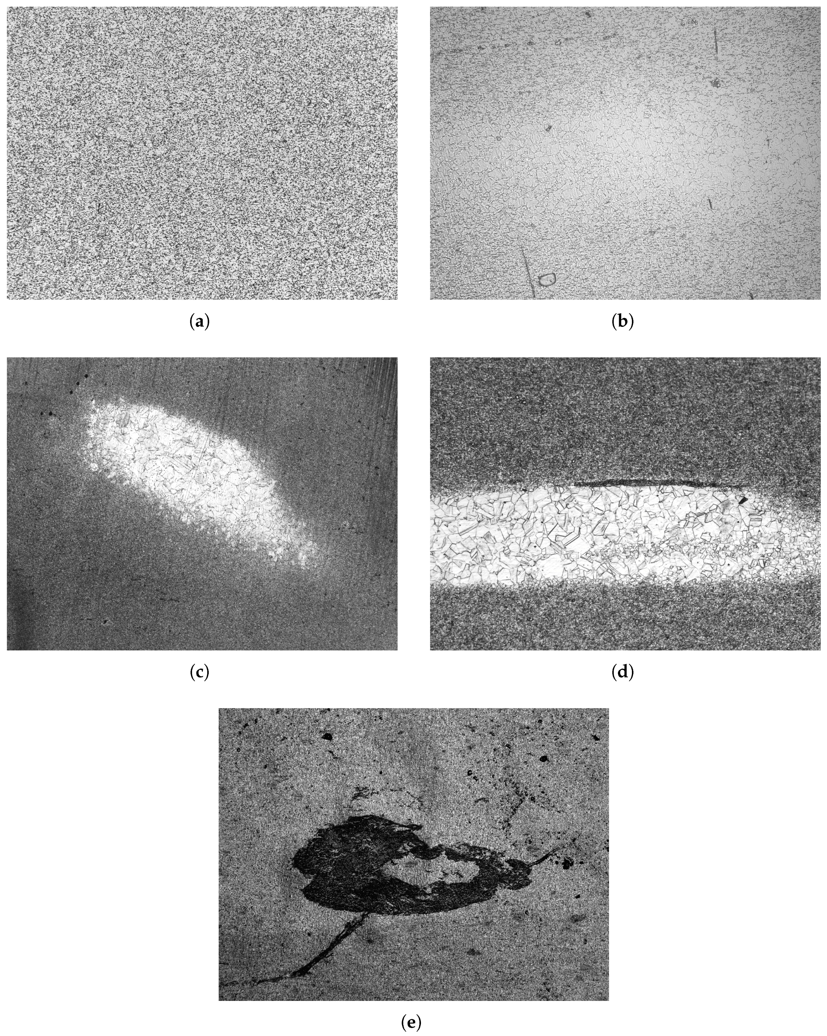
Figure 1. Prime example micrographs of each class: (a) Conform microstructure, (b) LEI, (c) CWS, (d) DWS, (e) NMI.
Metals 15 01172 g001
Figure 2. Synthetic data generation framework.
Metals 15 01172 g002
Figure 3. Macro-average test set F1 score of the model trained on the different datasets with its native performance, data augmentation, and the synthetic rebalancing.
Metals 15 01172 g003
Figure 4. Examples for the features most named by experts during the round robin test which indicated synthetic samples. The features are marked in the images by red boxes. (a) Artificial particle pattern in a inclusion. (b) Unnatural boundary shape and sharpness between matrix structure and coarse grain.
Metals 15 01172 g004
Figure 5. Percentage of samples identified correctly as real or synthetic and percentage of synthetic samples classified correctly in their indented defect class compared to the normal control samples in this class.
Metals 15 01172 g005
Figure 6. Quality percentage of the synthetic microstructure defects compared to the real control samples.
Metals 15 01172 g006
Table 1. Initial distribution of the data.
ClassesNumber of Samples
Conform140
LEI351
CWS209
DWS106
NMI110
Sum916
Table 2. Defect samples per class in the subsampled datasets to achieve several distinct ρ imbalance ratios.
ρ Samples per Defect ClassSamples in Conform ClassTotal Samples in the Dataset
1 (Balanced)8585425
24285253
51785153
10885117
20485101
Table 3. Contents of the four datasets which were rebalanced by the synthetic data generated with our framework.
ρ Real Samples per
Defect Class
Synthetic Samples per
Defect Class
Samples in Conform ClassTotal Samples in the Dataset
2424385425
5176885425
1087785425
2048185425
Table 4. Results of the model study.
ModelCross-Validation AccuracyModel Architecture Source
ConvNextBase0.72[59]
DenseNet1210.70[58]
DenseNet1690.75[58]
DenseNet2010.74[58]
EfficientNetV2B30.68[60]
EfficientNetV2L0.67[60]
InceptionV30.62[56]
RegNetX1200.71[61]
RegNetY0800.71[61]
RegNetY1200.73[61]
RegNetY1600.70[61]
ResNetRS2000.63[62]
ResNetV21010.69[63]
VGG190.69[64]
Xception0.68[65]
Table 5. Mean observed agreement, expected agreement, and Fleiss’ Kappa values for the two questions of the first part of the round robin test.
QuestionObserved
Agreement
Expected
Agreement
Fleiss’ Kappa
real/synthetic
recognition
0.730.530.42
defect classification0.820.300.74
Table 6. Standard deviation by class computed from the quality score given by the experts in the second part of the round robin test.
ClassStandard DeviationReal Control Samples Standard
Deviation
LEI0.8030.765
CWS1.0010.930
DWS0.7400.673
NMI0.7370.533
Table 7. Class-wise F1 score on the ρ = 2 dataset with the filtered synthetic samples.
ClassesTest Set F1 Score
Conform0.83
LEI0.57
CWS0.76
DWS0.74
NMI0.85
Disclaimer/Publisher’s Note: The statements, opinions and data contained in all publications are solely those of the individual author(s) and contributor(s) and not of MDPI and/or the editor(s). MDPI and/or the editor(s) disclaim responsibility for any injury to people or property resulting from any ideas, methods, instructions or products referred to in the content.