Optimization of Welded Joints under Fatigue Loadings

Abstract

In this paper, the notch effect in weldments has been investigated, and the optimal configuration of different types of welded joints has been analysed using the implicit gradient approach. By considering this implicit gradient method, it is possible to calculate the effective stress related to fatigue damage, with the effective stress being a continuous scalar function of the real stress tensor components, even in the presence of sharp edges. Hence, the search for the optimal configuration that maximises fatigue life can be tackled as the condition of minimum effective stress obtained by changing the weld shape and geometrical parameters. Both load-carrying cruciform joints and spot welds made of steel have been considered. The structural details have been studied by modelling actual shapes without any geometric simplification. Moreover, the same numerical procedure has been considered independently of the size, shape or load condition without imposing restrictive rules on the FE mesh.

1. Introduction

Welded joints are characterised by sharp V-notches at the weld toe or root, so that the linear elastic peak stress tends to infinity. The fatigue strength of welded structures is typically assessed using the nominal stress approach [1]. This approach is the main method used and is straightforward in its methodology: for a specific structural component, within the wide ranges of the welded details included in technical standards, its fatigue strength class is directly given by the standards and is expressed in terms of nominal stress. Consequently, the standards provide a collection of fatigue resistance curves, each having similar qualities but corresponding to structurally distinct details. The nominal stress method, specified by Eurocode 3 [1], proposes fatigue resistance curves as a function of nominal stress and is applicable to arc welding with different possible thicknesses of the main plate. The designer has control over the nominal stress and any drawbacks due to using thicknesses exceeding 25 mm or any other critical parameter or defect.

However, when dealing with large, complex welded structures, the application of nominal stress could present some difficulties. One of the possible problems could be the definition of actual or applicable nominal stress, particularly when joined structural elements are not simply beams or trusses [2,3]. Other problems could arise if the welded geometry is not in the collection given by design standards. Alternatively, a method related to local stresses should be employed to extend the resistance curves to a joint with a shape that is not classified by Eurocode. There are several methodologies in the literature that summarise fatigue resistance data for joints of a generic shape, and they are linked to a linear elastic approach [2]. These include the structural stress and hot spot methods [3,4,5,6,7], the notch stress approach [8,9,10,11,12], energetic approaches [13,14,15,16] and the peak stress method that simplifies the numerical approach [17,18]. Conversely, the authors have proposed the implicit gradient method, which solves the problem of calculating the effective stress σ_eff at every point of the weld bead using a single numerical post-processing of the Cauchy tensor operating in two- or three-dimensional components [19,20]. The method has been proven to be able to sum up several hundred pieces of experimental data related to different welded joints by considering different main plate thicknesses and shapes gathered together into a single scatter band [19,21]. The unique SN curve that is obtained for steel joints and its related scatter band have a slope equal to 3 and a reference value at 2 × 10⁶ cycles equal to 151 MPa at 97.7% survival probability. For aluminium alloys, the SN curve slope turns out to be 3.75, and the reference value at 2 × 10⁶ cycles is equal to 80 MPa. Moreover, as shown in reference [22], the effective stress σ_eff obtained with the implicit gradient method can be used to tackle the fatigue life assessment of spot-welded joints with thicknesses of a few millimetres or less. This result was achieved without modifying the general approach proposed in [19]. The spot weld is treated as a three-dimensional stress concentration problem. The effective stress is calculated around the entire contour of the welding point, highlighting how the areas of maximum effective stress concentration are a likely initiation point for fatigue cracks.

The continuous development of software tools and the improvement of computer performance allow for relatively fast three-dimensional Finite Element (FE) analyses of components, even in complex cases of welded details. This provides designers with the opportunity to use FE data for accurate structural verification and potentially improve existing solutions by leveraging optimisation concepts and mathematical techniques. The resolution of structural design problems is linked to the minimisation or maximisation of certain physical quantities of interest, primarily following three types of processes: topological optimisation, shape optimisation and parametric optimisation. In optimisation processes, it is customary to define an objective function to rationally evaluate the results of the process. Typically, the objective function represents the value of a characteristic quantity of the problem under consideration, such as the maximum principal stress induced by loads, the weight of the structure or its stiffness [23]. In most cases, the objective function is maximised or minimised by acting on the values of design variables that define the dimensions of the component (thickness of a plate, area of a section, position of a hole, etc.), either alternatively by acting on the properties of the material used (elastic modulus, yield strength, density, etc.) or by modifying any other quantity that defines the mechanical behaviour. However, constraints on control quantities must be defined to obtain physically acceptable results that are consistent (for example, a dimensional parameter must fall between a minimum and maximum value, a generic section must be greater than an assigned value, etc.). Additionally, a genetic algorithm should be used to optimise the structure of the artificial neural network related to fatigue life [24,25]. This innovative approach aims to reduce the number of required tests and the associated costs of conducting destructive tests while maintaining satisfactory reliability.

In this work, as an example of a two-dimensional optimisation of the weld size, cruciform load-carrying welded joints under tensile loading will be analysed. Furthermore, as a three-dimensional study, some examples of spot-welded joints will be studied to show the capabilities of the implicit gradient method in solving an optimisation problem within a predefined range of parameters. These structural configurations have been carefully examined without resorting to any geometrical simplifications, ensuring a comprehensive understanding of their fatigue behaviour. The analyses performed will refer to steel under mainly linear elastic behaviour without considering, at this preliminary stage, the contact problem related to the secondary bending or deflection of the joined plates.

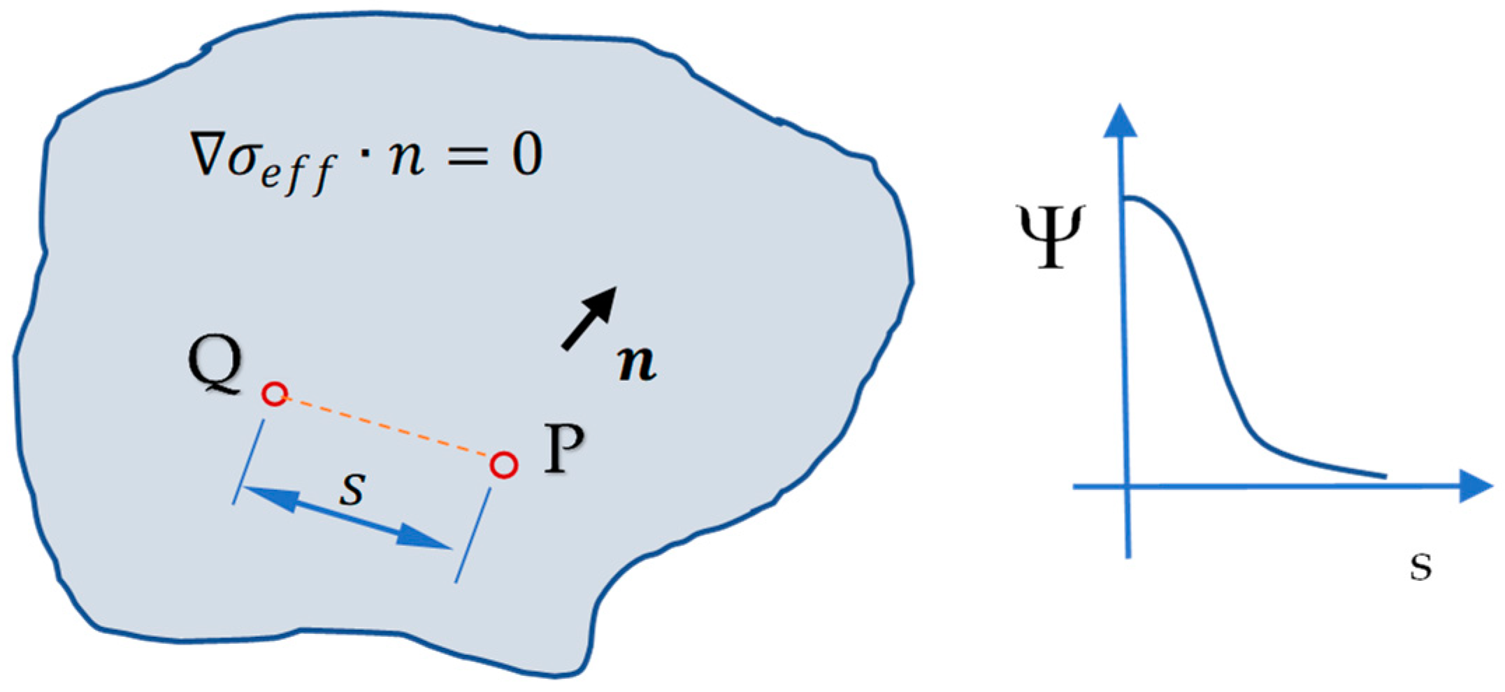
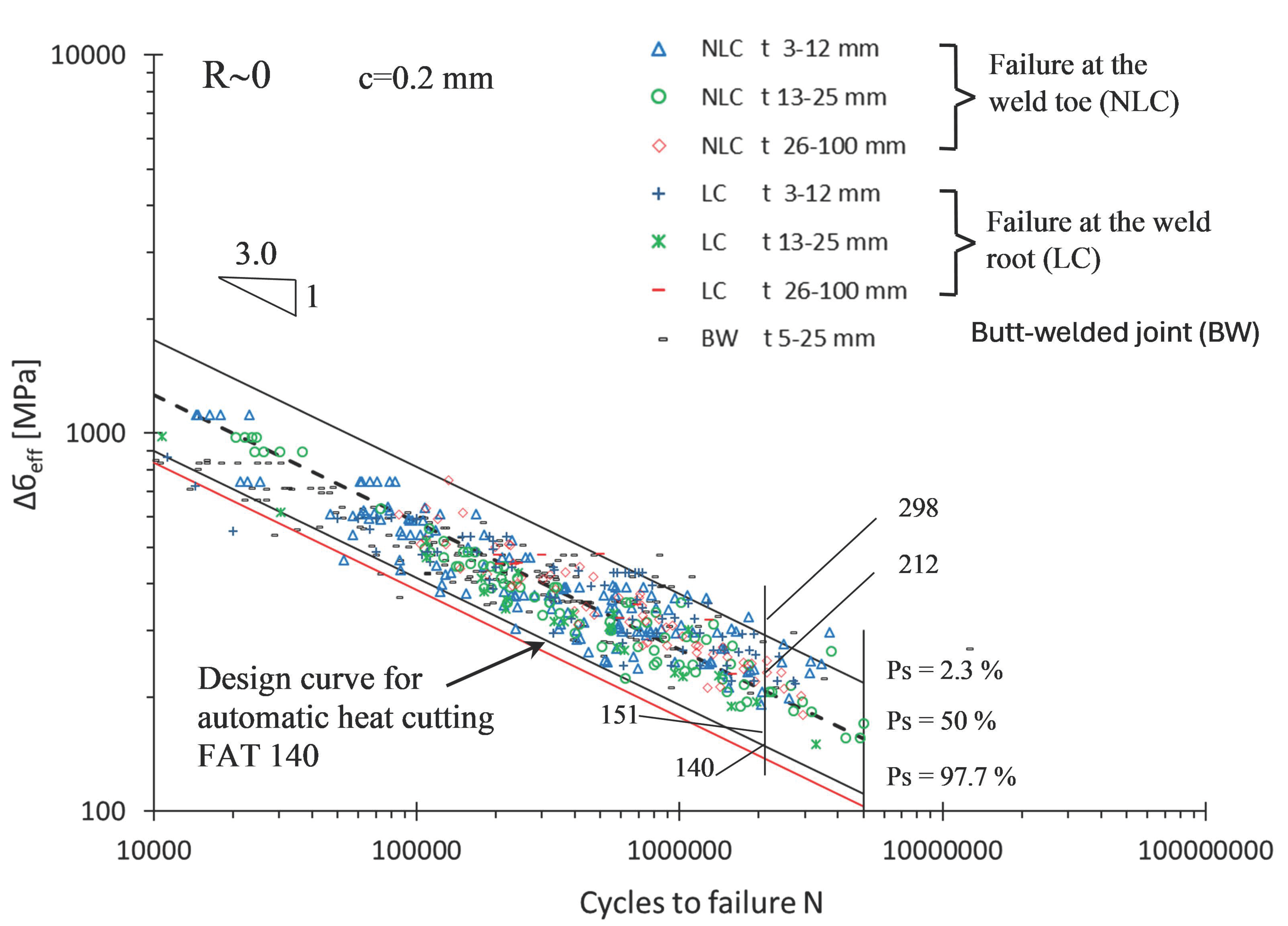
2. The Fatigue Strength Curve for Welds with the Implicit Gradient Method

The implicit gradient method posits that the fatigue behaviour of the material will be correlated with the average across the entire body of a physical quantity linked to the damage. A decreasing weight function ψ(P,Q) assigns greater importance to what happens in the immediate vicinity of a point than to what occurs at a distance. This approach makes it possible to overcome the issue of the singularity of the stress field near sharp edges.

The procedure is the following: when considering a continuous body of homogeneous material, loaded and constrained, with volume V, at each point of volume V, the internal forces induce a local stress tensor $\stackrel{̿}{\mathsf{\sigma }}$. For the strength assessment, the tensor is usually reduced to a local equivalent scalar value, σ_eq, according to a convenient strength criterion. The main principal stress value of the local stress tensor $\stackrel{̿}{\mathsf{\sigma }}$ is generally suitable under simple uniaxial loading on a welded structure; such an assumption is assumed in this paper. Under more complex, generally multiaxial, loadings, a different definition of σ_eq can be given by assuming a multiaxial criterion; the procedure can be easily upgraded.

At this point, a continuous local scalar with an equivalent value, σ_eq, is available all over the domain V. Depending on the geometry and boundaries, there could be singularities and/or general local stress raisers that are not directly related to overall strength. The implicit gradient, as well as any notch strength theory, deals with such a problem. In particular, it is possible to define an effective stress σ_eff at the generic point P in volume V. Such an effective value is usually defined as non-local because it depends on the gradients and stress values in the material surrounding point P.

In our case, the effective value is the integral average of local stress σ_eq, weighted by an appropriate weight function ψ(P,Q), which takes into account the distance s between the considered point P and the surrounding points Q (s = ‖PQ‖) [26,27].

The effective stress is defined as:

$${\sigma }_{eff}(P)=\frac{{\displaystyle \underset{V}{\int }\Psi (P,Q) {\sigma }_{eq}(Q) dV\hspace{1em}\hspace{1em}}}{{\displaystyle \underset{V}{\int }\Psi (P,Q) dV\hspace{1em}\hspace{1em}}}$$

(1)

where Q is any point inside volume V. Since any suitable choice of function ψ(P,Q) decreases with increasing distance s, the stress values too far from P are actually meaningless.

This “integral approach” of Equation (1) is a common approach to several “notch strength approaches”.

The peculiarity of the implicit gradient is that, in order to calculate σ_eff, instead of solving Equation (1) point by point as previously formulated, the integration is approximated by a Helmholtz differential equation within volume V of the component [28,29,30]:

$${\sigma }_{eff}-c^2{\nabla }^2{\sigma }_{eff}={\sigma }_{eq} in V$$

(2)

The parameter c that appears in Equation (2) is a characteristic length that governs the influence zone of the weight function ψ and is assumed to depend only on the material characteristics. For steel welds, c takes the value of 0.2 mm, whereas for aluminium alloys, c is equal to 0.15 mm [21]. ${\nabla }^2$ represents the Laplace operator.

To solve the non-homogeneous Helmholtz differential equation, the Neumann boundary condition is considered [21,29]:

$$\nabla {\sigma }_{eff} \cdot n=0 \hspace{1em} su \hspace{1em}\partial V$$

(3)

where n represents the outward normal to the boundary of V and $\nabla$ denotes the gradient operator (see Figure 1).

This approach opens up the opportunity to use the same calculation procedure for welds regardless of geometry, welding type and joint complexity without necessarily introducing simplifications in three-dimensional models, thus reducing design problems and costs [19,21,22].

After creating the three-dimensional model of the weld with a solid modelling tool, it is possible to perform FE analysis. Since the stress analysis is simply linear elastic for high-cycle fatigue strength assessment, the base metal, heat-affected zone and weld are considered to have the same elastic physical characteristics as is usually the case in the methods proposed in the literature [2,3]. Subsequently, using the same mesh, Equation (2) can be solved automatically with numerical integration software. For instance, in this paper, Comsol multiphysics software has been used.

Being an averaged value, σ_eff has smother gradients, so the numerical convergence of Equation (2) is easier than the initial linear elastic stress evaluation in the domain. Once the stress fields have been solved, σ_eff is substantially mesh-independent, or at least less mesh-dependent than the stress field evaluation.

In general, raw mesh is sufficient, and stable results are obtained with a low number of elements since an acceptable value of σ_eff can be obtained even if the stress components are not estimated exactly at every point of the considered domain at a local level. As a general rule, the size of the mesh in critical positions should be close to the characteristic length value c [22].

Figure 2 illustrates the profile of the effective stress in a non-load-carrying cruciform joint subjected to tensile loading, along with its corresponding computational mesh. The mesh has been refined only within the region of maximum gradient. As is well known, the peak stress of the maximum principal stress tends to be infinite [31]. On the contrary, at the weld toe, the effective stress assumes a discrete value because the effective stress results in a continuous function [29,32].

For welded joints, assuming that the maximum principal stress is damaging and using various sets of experimental data from the literature in reference [19], a universal scatter band for steel welds with a fatigue life ranging between 10⁴ and 5 × 10⁶ cycles has been obtained, as shown in Figure 3. The range of effective stress is found to be independent of the joint type, main plate size and load type. The slope of the Wöhler curve is approximately 3, and the reference value at 2 × 10⁶ cycles with a 97.7% survival probability is about 150 MPa. This particular slope reflects the intrinsic material behaviour and the mechanistic response of steel welds under constant cyclic loading conditions, as found by Haibach [33]. Once the fatigue strength is defined, it becomes straightforward to calculate the maximum value of the effective stress range to be applied to the joint for fatigue lives that are not lower than the imposed limit. Notably, the Wöhler curve, corresponding to a 97.7% survival probability, aligns closely with the design curve typical for joints created by automatic heat cutting, characterised by a FAT class of 140.

3. Optimisation of the Weld Bead Shape in Load-Carrying Cruciform Joints

For welded joints subjected to fatigue loading at constant amplitude, the value of the maximum effective stress range can be applied; consequently, the expected fatigue life is quickly calculated by means of the Wöhler SN curve in Figure 3. Needless to say, the fatigue life of welded joints increases when the effective stress decreases; therefore, geometry optimisation is related to the ability to keep the value of the effective stress low under the same applied external load.

The example of parametric structural optimisation considered in this section concerns typical load-carrying cruciform joints under tensile loading. One or more geometric parameters can optimise the shape of the weld and determine the initiation point of the fatigue cracks.

The analysed welded joints are shown in Figure 4a. In these cases, three-dimensional FEM analysis can be replaced by a two-dimensional analysis, assuming that the stress gradients in the thickness direction are negligible. Specifically, a plane-stress state is adopted. Furthermore, considering the constraints and geometric symmetries, only a quarter of the entire domain is modelled, as reported in Figure 4b. This allowed for advantages in terms of computational time.

Using the implicit gradient method mentioned above, a geometric configuration is now sought. It is adjusted by one or more parameters, which maximise the fatigue life of the analysed welded components. All simulations will use the maximum principal stress evaluated under linear elastic assumptions as the damaging stress, assuming a value of C equal to 0.2 mm for the material (steel) [21]. Furthermore, the presence of residual stresses induced by the welding process is neglected.

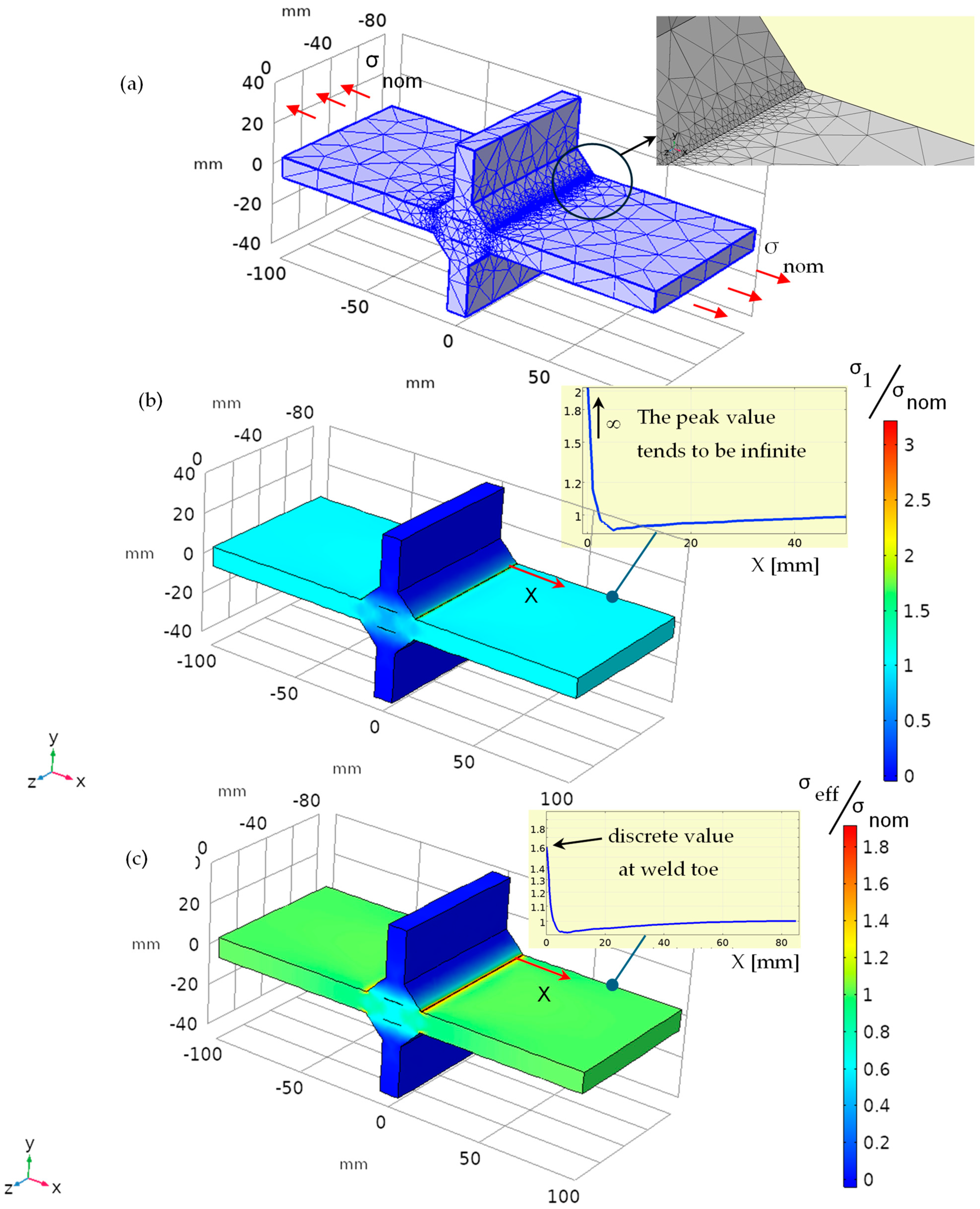
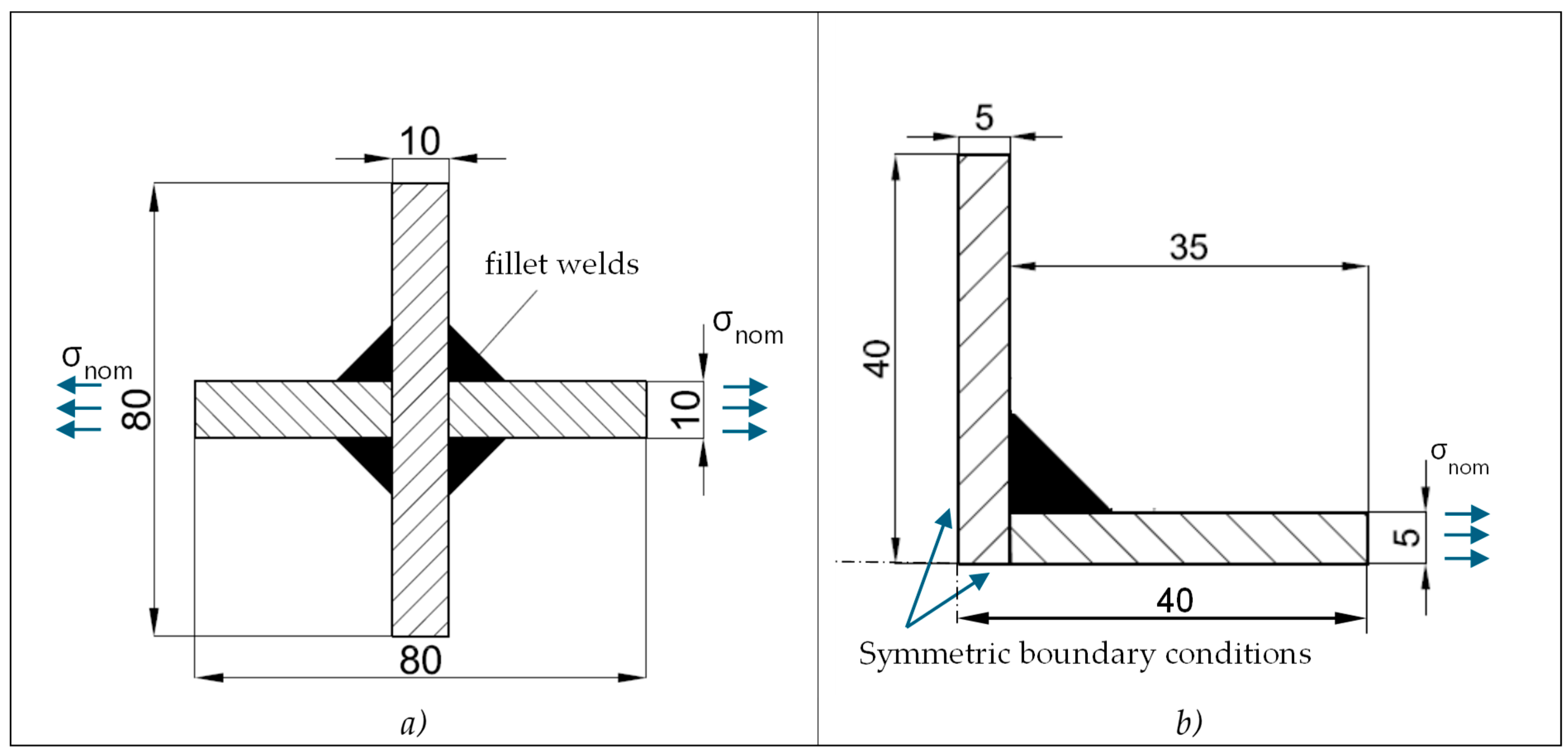
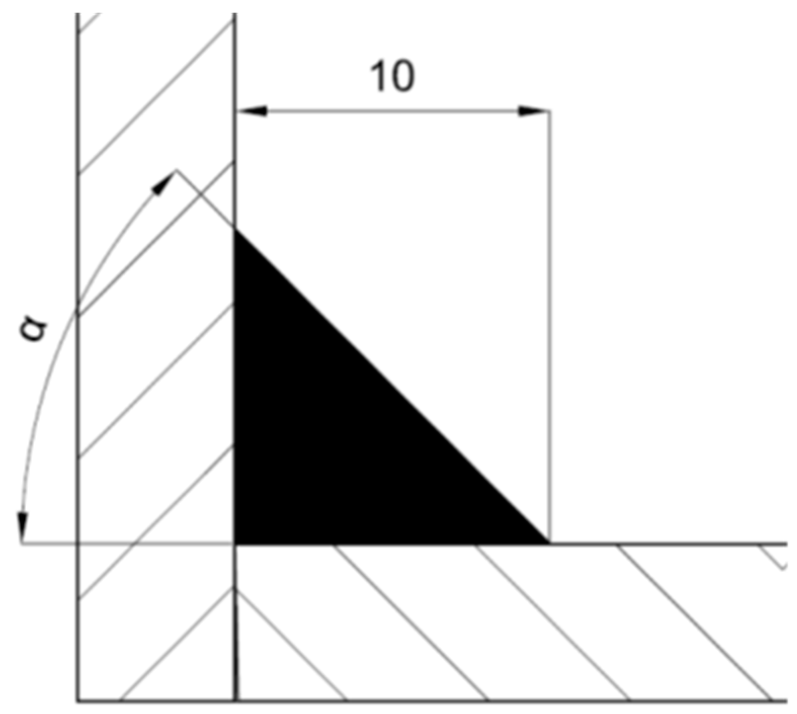
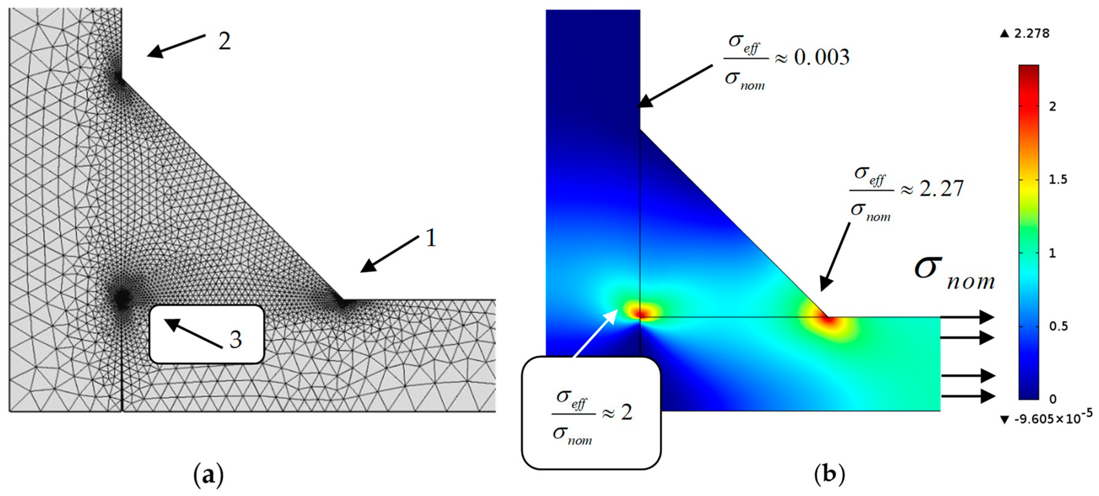
3.1. Weld Bead Optimisation in a Load-Carrying Cruciform Joint with Constant Weld Leg Length under Tensile Loading

In the first example considered, parameter α modifies the slope of the weld bead, relative to the main plate (see Figure 5). The objective of the optimisation is to evaluate the influence of angle α on the fatigue strength of the specimen in the case of a load-carrying configuration with constant weld leg length. The potential crack initiation points for fatigue are the three points indicated in Figure 6a: the two points at the weld toe (points 1 and 2) and the point at the weld root (point 3). With the implicit gradient method, the crack initiation zone is not predefined, but it is sufficient to check where the maximum value of the effective stress is obtained. This point is the preferred site for fatigue crack initiation. The mesh in Figure 6a has smaller elements with sizes around half a tenth of a millimetre and is sufficiently accurate to ensure a rapid calculation of the fatigue life in terms of effective stress σ_eff. It is not necessary to define a restrictive element size, but the operator shall lead the meshing program to have the smallest elements with sizes around a tenth of a millimetre near the toe or the root of the weld bead. In the example in Figure 6b, the maximum effective stress, which is normalised by the nominal tensile stress σ_nom, is 2.27 at the toe of the bead and 2 at the root. This means that the fracture initiation condition is more critical at the toe and that the crack is more likely to nucleate in that area.

Based on the FEM analyses performed on the joint in Figure 5, Figure 7 (left) shows that a value of parameter α of about 40° divides two zones: for α values less than 40°, the maximum effective stress is at the root, while for α values greater than 40°, the maximum shifts to the toe. The geometric configuration that equalises the effective stress at the toe of the weld bead with that at the root is shown in Figure 7 (right). Therefore, the optimal condition that minimises the effective stress while maintaining L involves an angle α close to 40°.

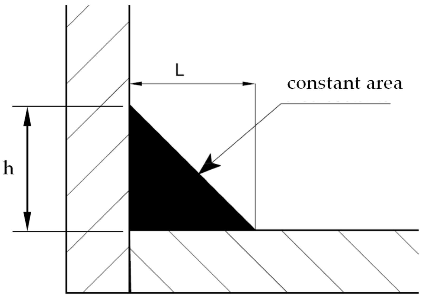
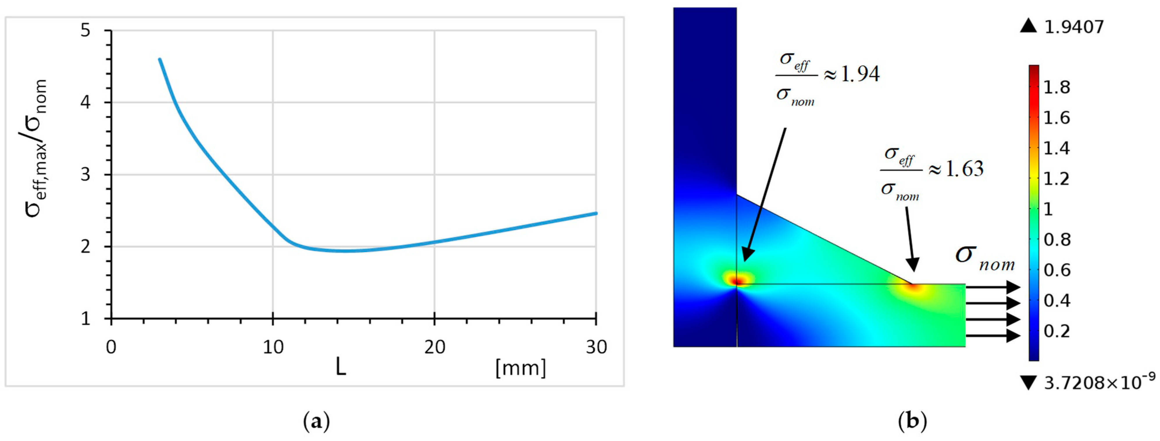
3.2. Weld Bead Optimisation in a Load-Carrying Cruciform Joint with a Constant Area of the Weld under Tensile Loading

This optimisation case refers to the model shown in Figure 8, subjecting the structure to tensile stress in the load-carrying configurations similarly to the previous case. The weld area is determined by the leg length L and height h of the horizontal side of the weld bead. Therefore, L is considered an independent variable, and h is calculated based on a predetermined weld area of 50 mm². This constraint forces alterations in the bead geometry to ensure a consistent volume of filler material used throughout the welding process.

In the load-carrying weld configuration, the optimal condition is achieved when the value of parameter L is close to 14 mm. The critical zone is at the root of the weld, where the value of effective stress σ_eff, normalised to nominal stress σ_nom, equals 1.94, as shown in Figure 9. For L values between 3 and 11 mm, however, the critical zone for fatigue cracking shifts to the toe.

4. Optimisation of Spot-Welded Joints

The fatigue analysis of spot-welded joints is critical in enhancing the performance of lightweight structures subjected to tensile and bending loadings [34,35,36]. These types of joints are extensively used across various industrial sectors, including automotive, aerospace and construction, due to their efficiency in force transmission and their ability to rapidly assemble different materials and components. Understanding the behaviour of spot-welded joints under cyclic loads is essential for predicting the lifespan of structures and preventing premature failure. This analysis encompasses the study of stress distribution, crack initiation, and propagation mechanisms at the micro and macro levels. By improving our knowledge of fatigue behaviour, it is possible to optimise the design and welding process, select appropriate materials and apply suitable treatments to extend the service life of lightweight structures while maintaining or reducing their weight.

The shape of the weld point, as normally outlined in three-dimensional models, is shown in Figure 10. Note that in Figure 10, no geometric exemplification has been applied in order to eliminate the singular stress field around the weld point [22]. On the contrary, the notch stress approach has to introduce a small tip radius in order to remove the stress singularity and then for the fatigue evaluation to reformulate the fatigue curve [9].

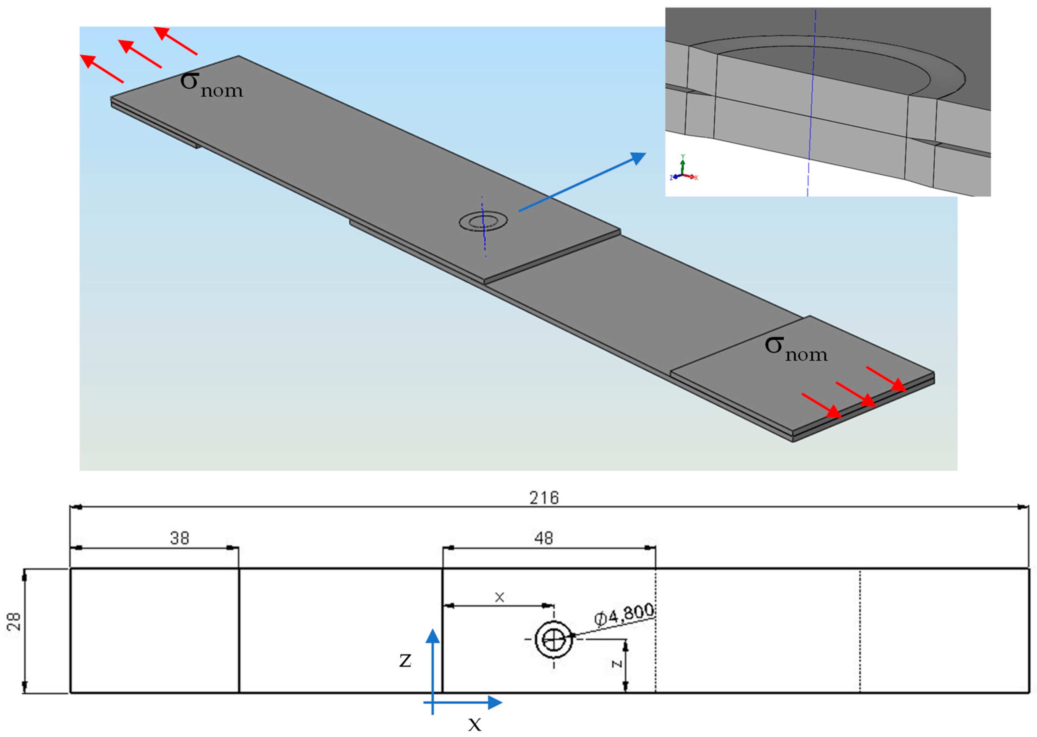
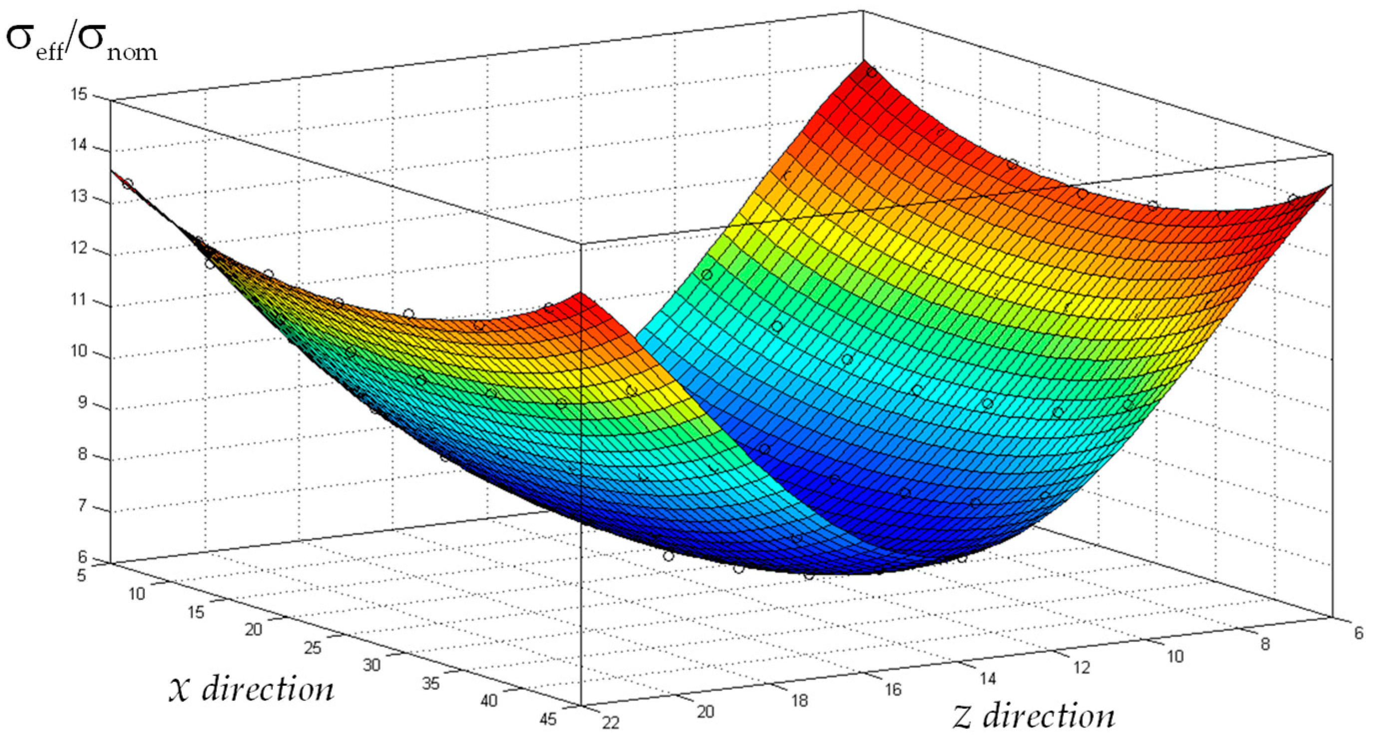
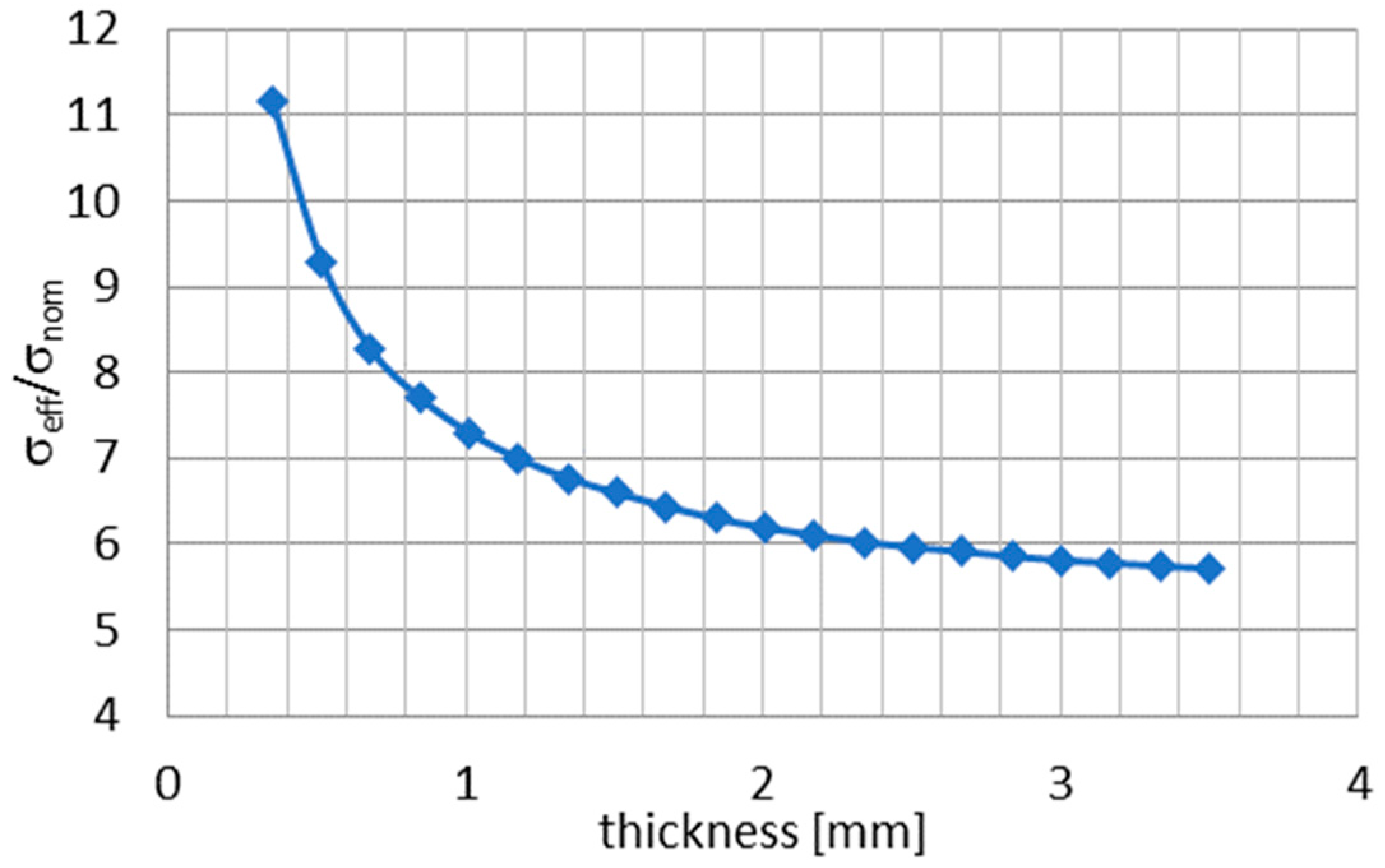
4.1. Lap Joint with a Single Weld Point

As a starting and preliminary test, the single spot weld is considered; the optimisation of a single spot position is actually reasonably easy. Figure 11 shows the specimen and the frame of reference considered for optimising the position of the weld point. The model reproduces the typical connection used in the literature to simulate the strength of spot-welded joints under external loadings [37,38,39,40]. The main size and shape of the model are shown in the figure. The weld spot position has free coordinates (x, z), and it is inevitably limited within the overlap area of the two plates. To simplify the analysis, the range for parameter x was divided into 7 intervals, while for the z direction, 10 discrete values were adopted in order to consider a total of 70 configurations.

The configuration with the lowest effective stress is obtained when the weld point is located in the central area of the overlap between the plates (x = 14 mm, z = 24 mm). Furthermore, it is clear that parameter z has a greater influence, as even modest variations in z result in significant increases in effective stress σ_eff. Conversely, a geometrical variation in the x direction causes smaller increments of the effective stress value. This effect is clearly visible in Figure 12. In other words, to achieve maximum strength, the weld point should be located on the longitudinal midline axis of the specimen so that no bending effects in the plane of the specimen occur.

The effect of the plate thickness is considered in Figure 13. Regarding the optimal configuration, the variation in thickness leads to a progressive reduction in σ_eff.

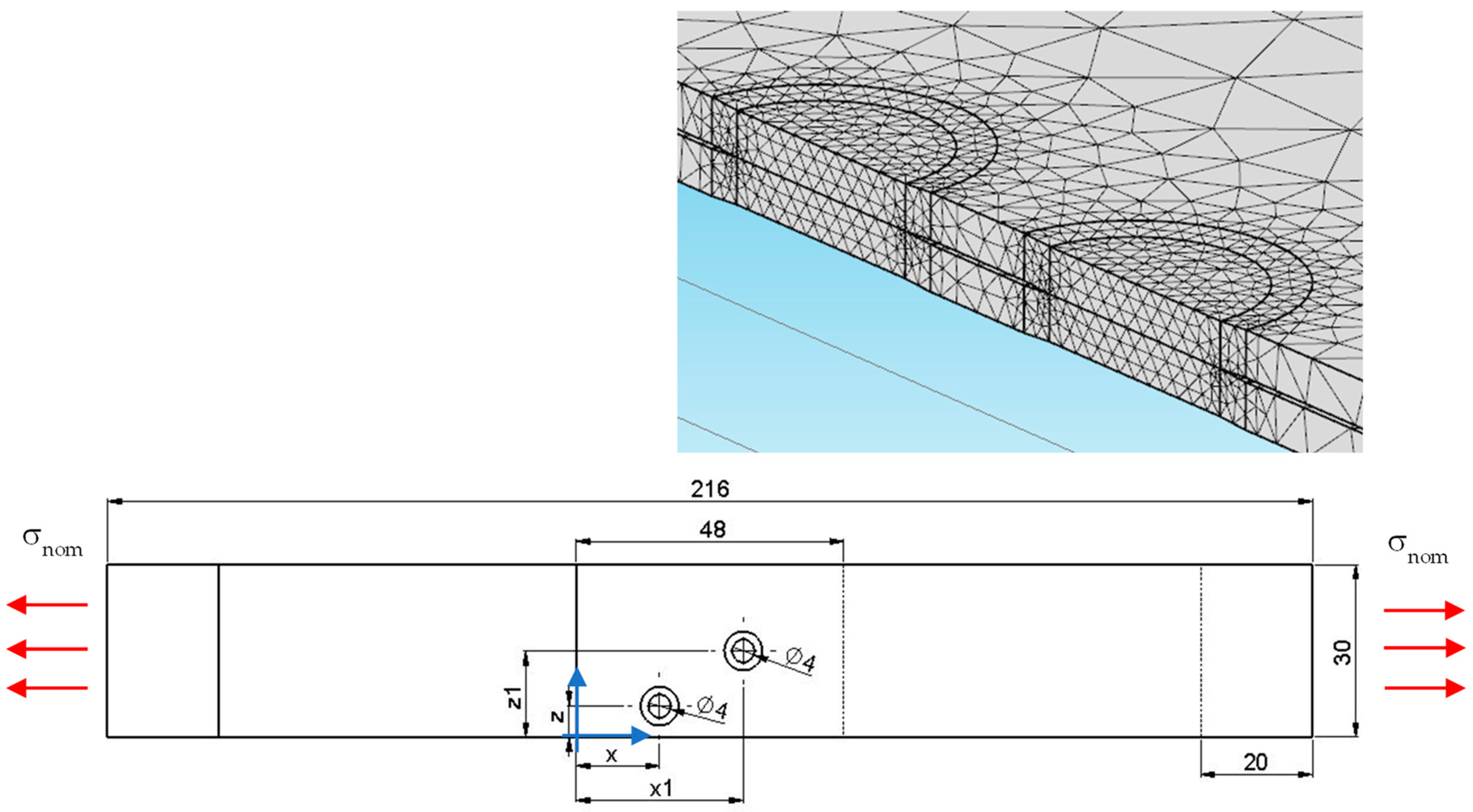
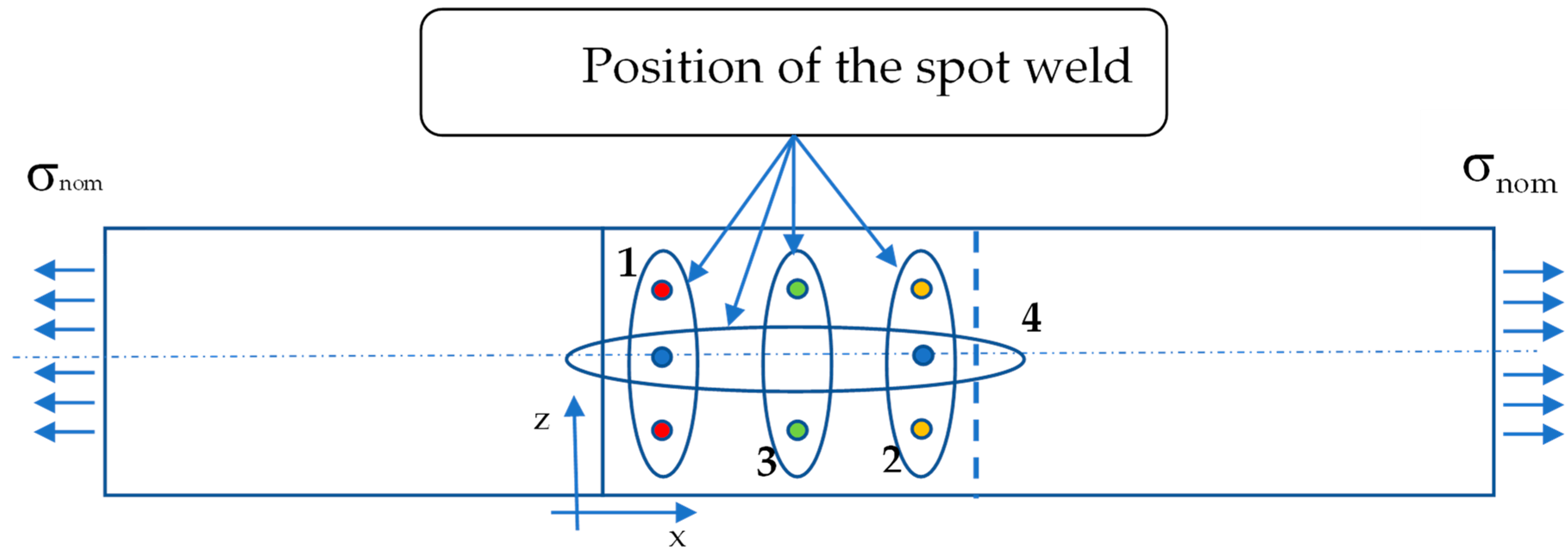
4.2. Lap Joint with Two Spot-Welded Points

In real applications, the actual problem is usually the position of several spots, so the second considered case is the optimisation of two spots. The specimen in Figure 14 has two weld points on the overlap area of the plates that can be moved by adjusting the parameters (x_i, z_i). Clearly, overlapping the two weld points should be avoided. In order to simplify the calculation, only three positions in both the x and z directions have been considered.

As in the previous case, the specimen is subjected to simple tensile loading.

The values of the maximum effective stress relative to nominal stress σ_eff/σ_nom obtained in the numerical analyses vary from a maximum of about 9 to a minimum of about 5.4. Only 4 of the combinations considered result in an σ_eff/σ_nom ratio lower than 6. Figure 15 shows the positions of the best four pairs of points.

Figure 15 illustrates that the optimal condition is achieved through a symmetric distribution of weld points along the longitudinal axis of the specimen, which is crucial for preventing in-plane bending. Notably, the effective stress values obtained from pairs of points 1, 2 and 3 are remarkably similar, highlighting the significance of this symmetrical arrangement.

Subsequent research has revealed that the optimal positioning of the points along the z-axis involves setting their distance apart to half the width of the specimen for each pair (1, 2 and 3).

Table 1. Optimal position for configuration 1 in Figure 15 to minimise the σ_eff/σ_nom ratio.

Position
x [mm]	7
z [mm]	7.2
x1 [mm]	7
z1 [mm]	22.5

presents the results, using accurate meshes similar to those employed in determining the optimal positions shown in Figure 14. The distances documented in the table correspond to the analysis of configuration 1, where the separation between the weld points is roughly 50% of the width of the specimen. Specifically, from Table 1, the distance between the points is approximately 15 mm for a sheet with a width of 30 mm.

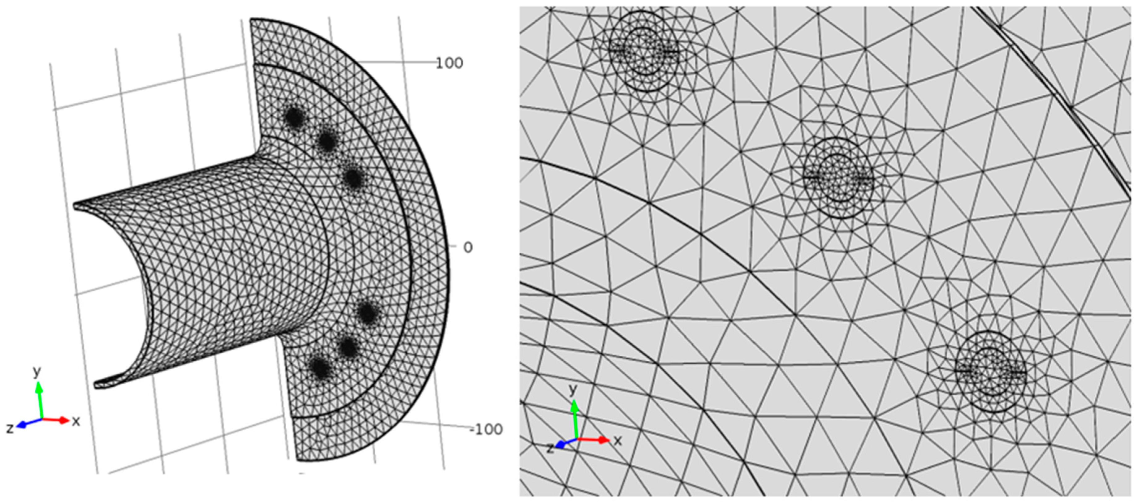
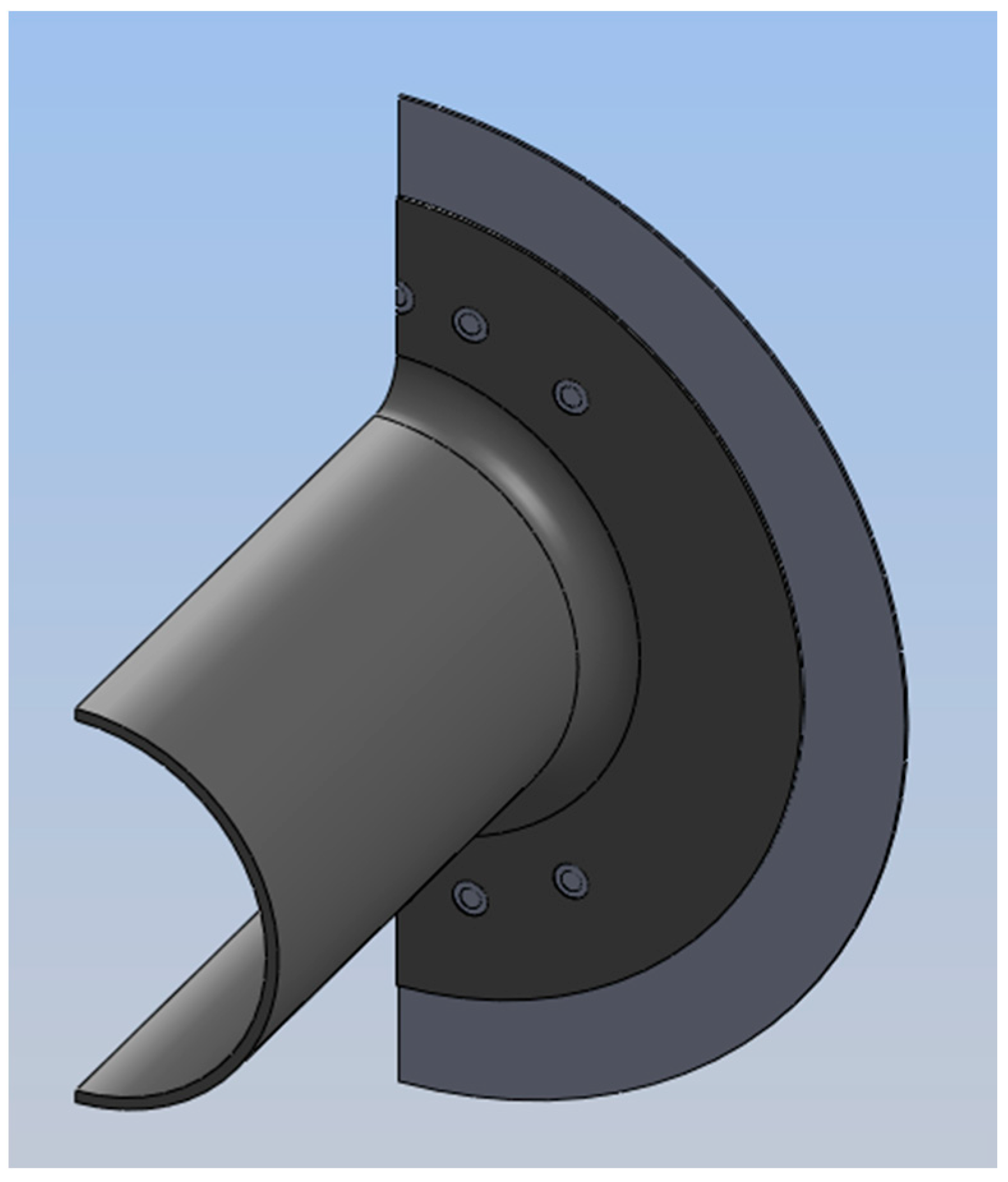
4.3. Tubular T Joints under Bending

The structures reported in Figure 16 and Figure 17 show the cases of a T-joint obtained by spot-welding; the weld points are positioned at the same distance from the axis of the tube (tube perpendicular to a sheet metal disc).

As in the previous cases, the optimisation method involves using a solid model with parametric dimensions, which allows for rapid modification of the arrangement of the weld points by adjusting the parameters.

To speed up the analysis, the weld points are arranged symmetrically (modifying the positions of the points in the first quadrant and taking advantage of the symmetry along the vertical and horizontal axes). This approach yields a series of results corresponding to a given combination of the geometric parameters α_i, evaluating the arrangement that optimises the structure in terms of fatigue resistance.

Referring to Figure 16, the three weld points, each with a diameter of 5 mm located in the first quadrant, are transferred along a fixed circumference with a diameter of 150 mm. Parameters α_i are varied, while the external load F at the extremity is kept constant.

The explored angles α_i ranged from 5 to 85 degrees, divided into 9 intervals. Within the limits of the considered discretisation, the optimal configuration was found to be α₁ = 5°, α₂ = 23° and α₃ = 41°.

Additionally, the scenario where the first welded point is fixed on the axis of symmetry (α₁ = 0° in Figure 18) was analysed. In this case, the optimal condition is achieved with α₂ = 14° and α₃ = 35°.

It is worth noting that in both scenarios, the optimal configuration does not coincide with the configuration that maximises the static moment of the weld points relative to the bending axis. This is because the three-dimensional FE model is capable of accounting for the notch effect caused by the weld points.

5. Conclusions

The implicit gradient method has emerged as a highly versatile numerical methodology capable of addressing parametric optimisation problems. Its flexibility in calculating the effective stress at every point of the component under examination enables the identification of the optimal configuration for constant-amplitude fatigue loadings. This optimal configuration is characterised by the geometric arrangement in which the effective stress reaches its minimum value at the weld toe or root. Specifically, in the case of cruciform welds, this method facilitates the determination of whether fatigue stress defect nucleation occurs at the weld toe or root, thereby enhancing fatigue resistance. For spot weld lap joints subjected to tensile stress, symmetric configurations offer superior fatigue resistance. The numerical results obtained are stable and independent of the mesh utilised, achieving rapid convergence. This opens up the possibility of applying the implicit gradient method for optimisation calculations regardless of the weld bead shapes and complexity of the joint without the need for simplifications in three-dimensional models. Consequently, this approach can significantly reduce the overall cost of design and offers a robust framework for the design and analysis of welded assemblies with improved fatigue life.

References

1. Eurocode 3; Design of Steel Structures; General Rules; CEN: Brussels, Belgium, 1993.
2. Radaj, D.; Sonsino, C.M.; Fricke, W. Fatigue Assessment of Welded Joints by Local Approaches, 2nd ed.; Woodhead Publishing: Cambridge, UK; CRC Press: Boca Raton, FL, USA, 2006. [Google Scholar]
3. Hobbacher, A. Recommendations for Fatigue Design of Welded Joints and Components; Document XIII-1823e07/XV-1254-07; IIW International Institute of Welding: Paris, France, 2007. [Google Scholar]
4. Niemi, E. Recommendations Concerning Stress Determination for Fatigue Analysis of Welded Components; IIW Doc. XIII-1458-92/XV-797-92; IIW International Institute of Welding: Paris, France, 1992. [Google Scholar]
5. Karabulut, B.; Rossi, B. On the applicability of the hot spot stress method to high strength duplex and carbon steel welded details. Eng. Fail. Anal. 2021, 128, 105629. [Google Scholar] [CrossRef]
6. Zhou, F.; Chen, Y.; Wang, W.; Xie, W.; Ying, T.; Yue, G. Investigation of hot spot stress for welded tubular K-joints with stiffeners. J. Constr. Steel Res. 2002, 197, 107452. [Google Scholar] [CrossRef]
7. Yu, Y.; Liu, Y.; Jiang, W.; Pei, X.; Wang, P.; Dong, P.; Wang, B.; Xie, X. Notch structural stress theory: Part II predicting total fatigue lives of notched structures. Int. J. Fatigue 2024, 182, 108201. [Google Scholar] [CrossRef]
8. Radaj, D. Design and Analysis of Fatigue Resistant Welded Structures; Abbington Publishing: Cambridge, UK, 1990. [Google Scholar]
9. Sonsino, C.M.; Baumgartner, J.; Breitenberger, M. Equivalent stress concepts for transforming of variable amplitude into constant amplitude loading and consequences for design and durability approval. Int. J. Fatigue 2022, 162, 106949. [Google Scholar] [CrossRef]
10. Ng, C.T.; Sonsino, C.M.; Susmel, L. Multiaxial fatigue assessment of welded joints: A review of Eurocode 3 and International Institute of Welding criteria with different stress analysis approaches. Fatigue Fract. Eng. Mater. Struct. 2024, 1–34. [Google Scholar] [CrossRef]
11. Karakaş, Ö.; Baumgartner, J.; Susmel, L. On the use of a fictitious notch radius equal to 0.3 mm to design against fatigue welded joints made of wrought magnesium alloy AZ31. Int. J. Fatigue 2020, 139, 105747. [Google Scholar] [CrossRef]
12. Glienke, R.; Kalkowsky, F.; Hobbacher, A.F.; Holch, A.; Thiele, M.; Marten, F.; Kersten, R.; Henkel, K.-M. Evaluation of the Fatigue Resistance of Butt-Welded Joints in Towers of Wind Turbines—A Comparison of Experimental Studies with Small Scale and Component Tests as Well as Numerical Based Approaches with Local Concepts. Weld. World 2024, 68, 1143–1168. [Google Scholar] [CrossRef]
13. Lazzarin, P.; Zambardi, R. A finite-volume-energy based approach to predict the static and fatigue behavior of components with sharp V-shaped notches. Int. J. Fract. 2001, 112, 275–298. [Google Scholar] [CrossRef]
14. Livieri, P.; Lazzarin, P. Fatigue strength of steel and aluminium welded joints based on generalised stress intensity factors and local strain energy values. Int. J. Fract. 2005, 133, 247–276. [Google Scholar] [CrossRef]
15. Schuscha, M.; Leitner, M.; Stoschka, M.; Meneghetti, G. Local strain energy density approach to assess the fatigue strength of sharp and blunt V-notches in cast steel. Int. J. Fatigue 2020, 132, 105334. [Google Scholar] [CrossRef]
16. Shoda, K.; Arai, K.; Nakamura, S.; Okada, H. Application of redefined J-integral range ΔJ for ultra-low cycle fatigue problems with large magnitude of elastic-plastic deformation. Theor. Appl. Fract. Mech. 2023, 126, 103938. [Google Scholar] [CrossRef]
17. Meneghetti, G.; Campagnolo, A. State-of-the-art review of peak stress method for fatigue strength assessment of welded joints. Int. J. Fatigue 2020, 139, 105705. [Google Scholar] [CrossRef]
18. Visentin, A.; Campagnolo, A.; Meneghetti, G. Analytical expressions to estimate rapidly the notch stress intensity factors at V-notch tips using the Peak Stress Method. Fatigue Fract. Eng. Mater. Struct. 2022, 46, 1572–1595. [Google Scholar] [CrossRef]
19. Tovo, R.; Livieri, P. An implicit gradient application to fatigue of sharp notches and weldments. Eng. Fract. Mech. 2007, 74, 515–526. [Google Scholar] [CrossRef]
20. Livieri, P.; Tovo, R. Overview of the geometrical influence on the fatigue strength of steel butt welds by a nonlocal approach. Fatigue Fract. Eng. Mater. Struct. 2020, 43, 502–514. [Google Scholar] [CrossRef]
21. Livieri, P.; Tovo, R. Fatigue strength of aluminium welded joints by a non-local approach. Int. J. Fatigue 2021, 143, 106000. [Google Scholar] [CrossRef]
22. Tovo, R.; Livieri, P. A numerical approach to fatigue assessment of spot weld joints. Fatigue Fract. Eng. Mater. Struct. 2011, 34, 32–45. [Google Scholar] [CrossRef]
23. Allaire, G.; Craig, A. Numerical Analysis and Optimization: An Introduction to Mathematical Modelling and Numerical Simulation; Oxford University Press: New York, NY, USA, 2007. [Google Scholar]
24. Amiri, N.; Farrahi, G.H.; Kashyzadeh, K.R.; Chizari, M. Applications of ultrasonic testing and machine learning methods to predict the static & fatigue behavior of spot-welded joints. J. Alloys Compd. 2020, 980, 173664. [Google Scholar]
25. Yu, Z.; Ma, N.; Murakawa, H.; Watanabe, G.; Liu, M.; Ma, Y. Prediction of the fatigue curve of high—Strength steel resistance spot welding joints by finite element analysis and machine learning. Int. J. Adv. Manuf. Tech. 2023, 128, 63–2779. [Google Scholar] [CrossRef]
26. Pijaudier-Cabot, G.; Bažant, Z.P. Nonlocal Damage Theory. J. Eng. Mech. 1987, 10, 1512–1533. [Google Scholar] [CrossRef]
27. Bažant, Z.P. Imbrigate continuum and its variational derivation. J. Eng. Mech. Div. ASCE 1984, 110, 1693–1712. [Google Scholar] [CrossRef]
28. Peerlings, R.H.J.; de Borst, R.; Brekelmans, W.A.M.; de Vree, J.H.P. Gradient enhanced damage for quasi-brittle material. Int. J. Numer. Methods Eng. 1996, 39, 3391–3403. [Google Scholar] [CrossRef]
29. Peerlings, R.H.J.; Geers, M.G.D.; de Borst, R.; Brekelmans, W.A.M. A critical comparison of nonlocal and gradient-enhanced softening continua. Int. J. Solids Struct. 2001, 38, 7723–7746. [Google Scholar] [CrossRef]
30. Aifantis, E.C. Update on a class of gradient theories. Mech. Mater. 2003, 35, 259–280. [Google Scholar] [CrossRef]
31. Williams, M.L. Stress singularities resulting from various boundary conditions in angular corners of plates in extension. J. Appl. Mech. 1952, 19, 526–528. [Google Scholar] [CrossRef]
32. Tovo, R.; Livieri, P. An implicit gradient application to fatigue of complex structures. Eng. Fract. Mech. 2008, 75, 1804–1814. [Google Scholar] [CrossRef]
33. Haibach, E. Service Fatigue-Strength—Methods and Data for Structural Analysis; VDI-Verlag: Dusseldorf, Germany, 1989. [Google Scholar]
34. Sakaguchi, M.; Kurokawa, Y.; Nakamura, F.; Hashimura, T. Fatigue strength of steel–aluminum alloy dissimilar lap joints fabricated by dimple spot welding for automotive application. Fatigue Fract. Eng. Mater. Struct. 2024, 47, 939–951. [Google Scholar] [CrossRef]
35. Yang, L.; Yang, B.; Yang, G.; Xiao, S.; Zhu, T.; Wang, F. A comparative study of fatigue estimation methods for single-spot and multispot welds. Fatigue Fract. Eng. Mater. Struct. 2020, 43, 1142–1158. [Google Scholar] [CrossRef]
36. Tanegashima, R.; Ohara, I.; Akebono, H.; Kato, M.; Sugeta, A. Cumulative fatigue damage evaluations on spot-welded joints using 590 MPa-class automobile steel. Fatigue Fract. Eng. Mater. Struct. 2015, 38, 870–879. [Google Scholar] [CrossRef]
37. Pan, N.; Sheppard, S. Spot welds fatigue life prediction with cyclic strain range. Int. J. Fatigue 2002, 24, 519–528. [Google Scholar] [CrossRef]
38. Long, X.; Khanna, S.K. Fatigue properties and failure characterization of spot welded high strength steel sheet. Int. J. Fatigue 2007, 29, 879–886. [Google Scholar] [CrossRef]
39. Lin, S.-H.; Pan, J.; Wung, P.; Chiang, J. A fatigue crack growth model for spot welds under cyclic loading conditions. Int. J. Fatigue 2006, 28, 792–803. [Google Scholar] [CrossRef]
40. Gao, Y.; Chucas, D.; Lewis, C.; McGregor, I.J. Rewiew of CAE fatigue analysis techniques for spot-welded high strength steel automotive structures. In SAE 2001 World Congress; 2001-01-0835; SAE Transactions: Warrendale, PA, USA, 2001. [Google Scholar]
Figure 1. Reference frame and Neumann boundary condition.
Metals 14 00613 g001
Figure 2. Effective stress σeff for a non-load carrying cruciform joint evaluated by solving Equation (2), assuming σeq coincides with the maximum principal stress σ1. The plate is subjected to a nominal tensile stress σnom; (a) mesh; (b) maximum principal stress σ1; (c) effective stress σeff.
Metals 14 00613 g002
Figure 3. Scatter band of steel welded joints (reprinted from Ref. [14]) of about 600 experimental points in terms of maximum effective stress range (scatter bands related to mean values plus/minus 2 standard deviations; NLC: non-load-carrying joint, LC: load-carrying joint, BW: butt-welded joint).
Metals 14 00613 g003
Figure 4. (a) Load-carrying cruciform joints under tensile loading; (b) Quarter model considered in the FE analysis.
Metals 14 00613 g004
Figure 5. Optimisation of parameter α while keeping L constant.
Metals 14 00613 g005
Figure 6. (a) Mesh used in the FE analysis (α = 45°); (b) non-dimensional effective stress.
Metals 14 00613 g006
Figure 7. (left) Effective stress against α; (right) Optimal configuration for α equal to 40°.
Metals 14 00613 g007
Figure 8. Optimisation keeping the constant area.
Metals 14 00613 g008
Figure 9. (a) Maximum non-dimensional effective stress against L; (b) Non-dimensional effective stress for optimal configuration with L = 14 mm and α = 27°.
Metals 14 00613 g009
Figure 10. Three-dimensional model for a spot weld.
Metals 14 00613 g010
Figure 11. Three-dimensional spot weld model and specimen size (d: spot weld diameter = 4.8 mm; t: plate thickness = 1 mm; σnom: tensile nominal stress).
Metals 14 00613 g011
Figure 12. Non-dimensional effective stress σeff as a function of (x, z) coordinates of the spot weld of Figure 11.
Metals 14 00613 g012
Figure 13. Effect of plate thickness on effective stress when the weld point is in the middle of the plate.
Metals 14 00613 g013
Figure 14. Specimen size and typical mesh for two spot welds (d: spot weld diameter = 4 mm; t: plate thickness = 1 mm; σnom: tensile nominal stress).
Metals 14 00613 g014
Figure 15. Positions where the σeff/σnom are less than 6.
Metals 14 00613 g015
Figure 16. Size and loading schematic diagram of the T-joint subjected to bending (size in millimetres).
Metals 14 00613 g016
Figure 17. Meshes used for the analysis of a T-joint subjected to bending stress.
Metals 14 00613 g017
Figure 18. View of the T-joint subjected to bending with the first welded point positioned on the symmetry axis (plate thickness and dimensions as indicated in Figure 16, α1 = 0°, α2 = 14° and α3 = 35°).
Metals 14 00613 g018