Non-Contact Evaluation of Deformation Characteristics on Automotive Steel Sheets


Abstract
1. Introduction
- -
- allow monitoring the course of the entire test,
- -
- allow for measuring more significant deformations,
- -
- provide information not only about one measured length but about the whole measured area,
- -
- they can also be used during tests at elevated temperatures.
2. Materials and Methods
- -
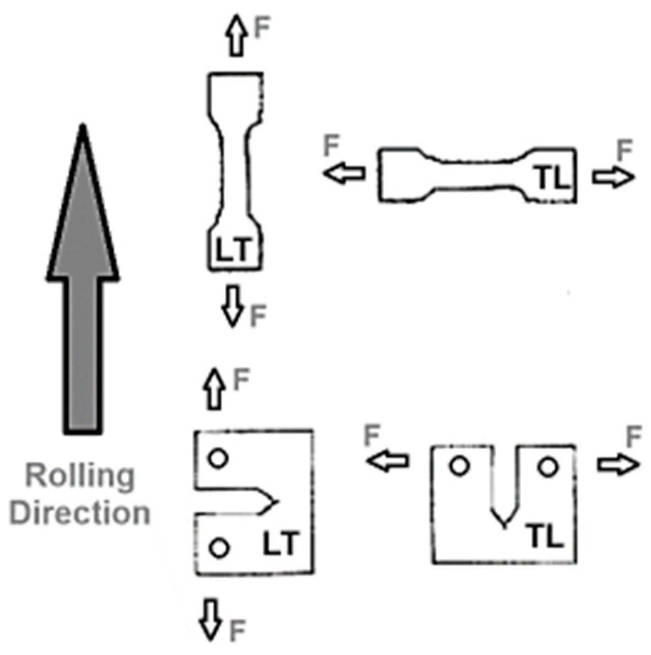
- specimen orientation LT—loading is parallel to the rolling direction; cracks will propagate perpendicular to RD;
- -
- specimen orientation TL—loading is perpendicular to the rolling direction, and the crack will propagate parallel to RD.
2.1. Materials
The Description of the Materials
2.2. Stable Crack Growth
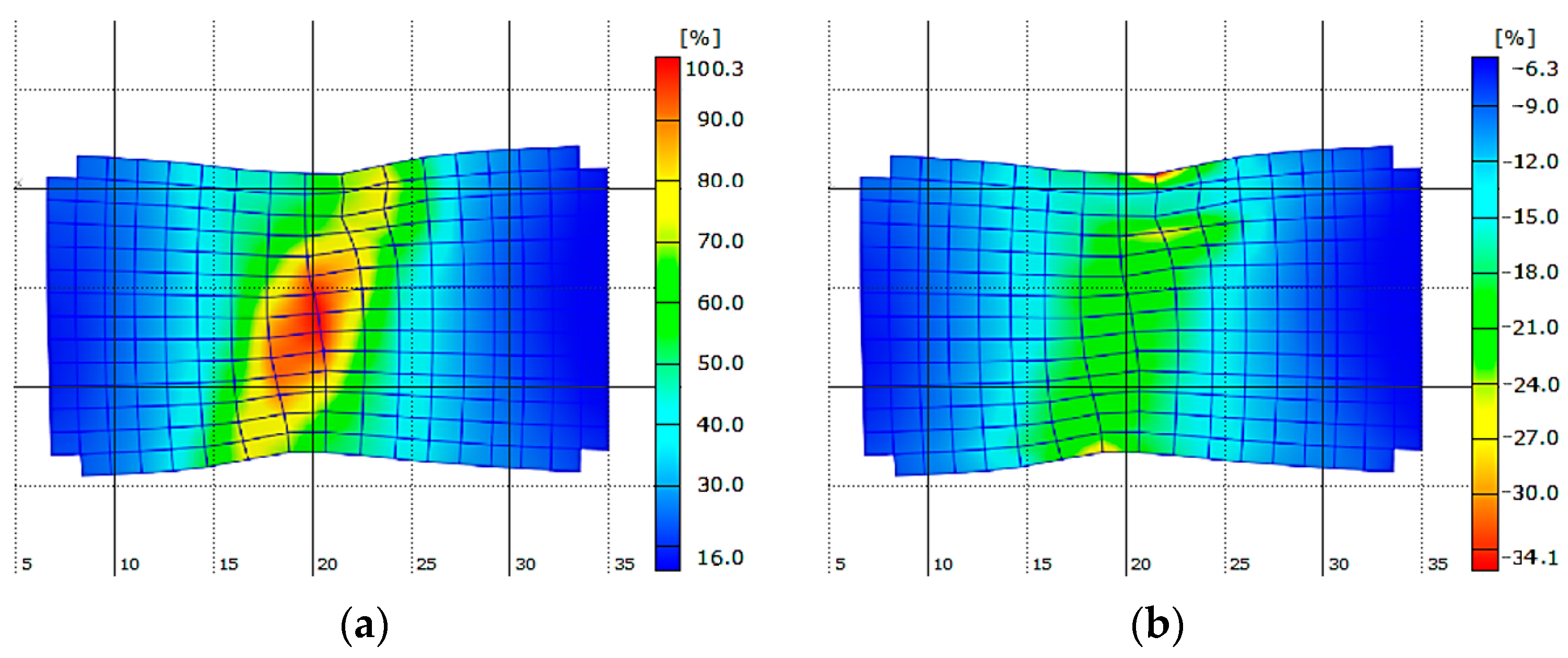
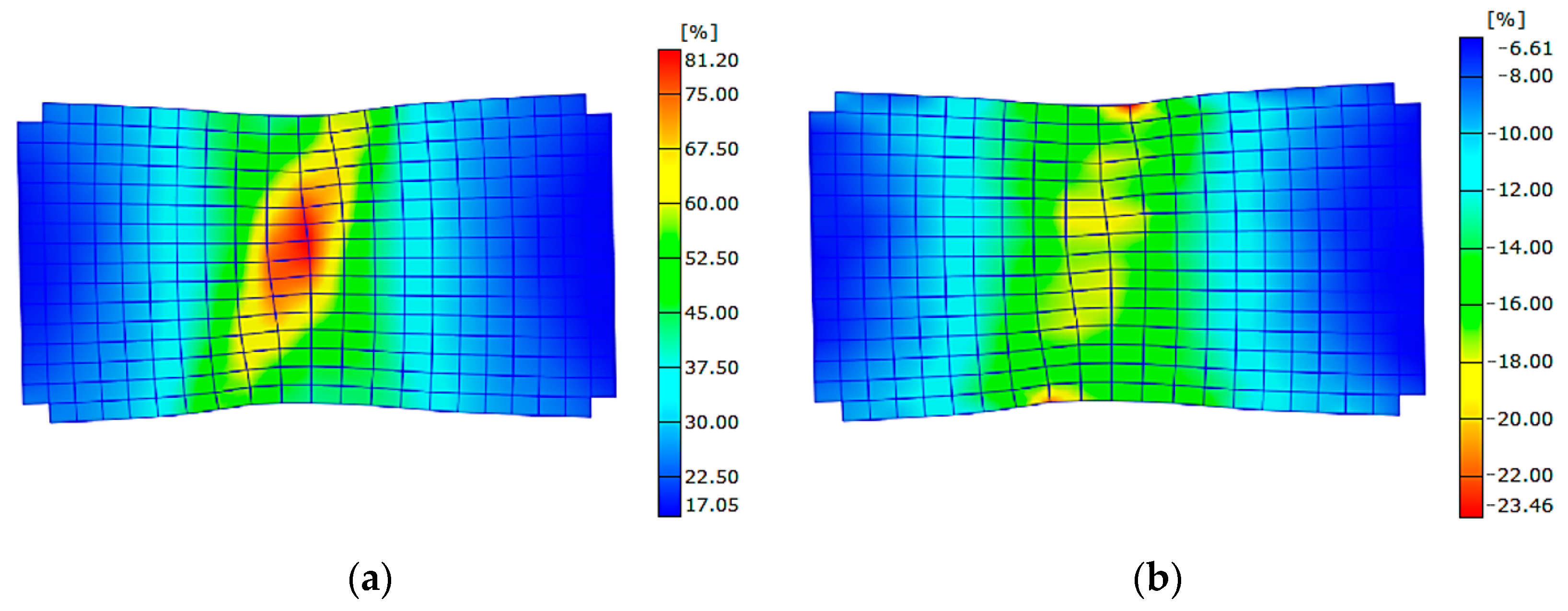
2.3. DIC
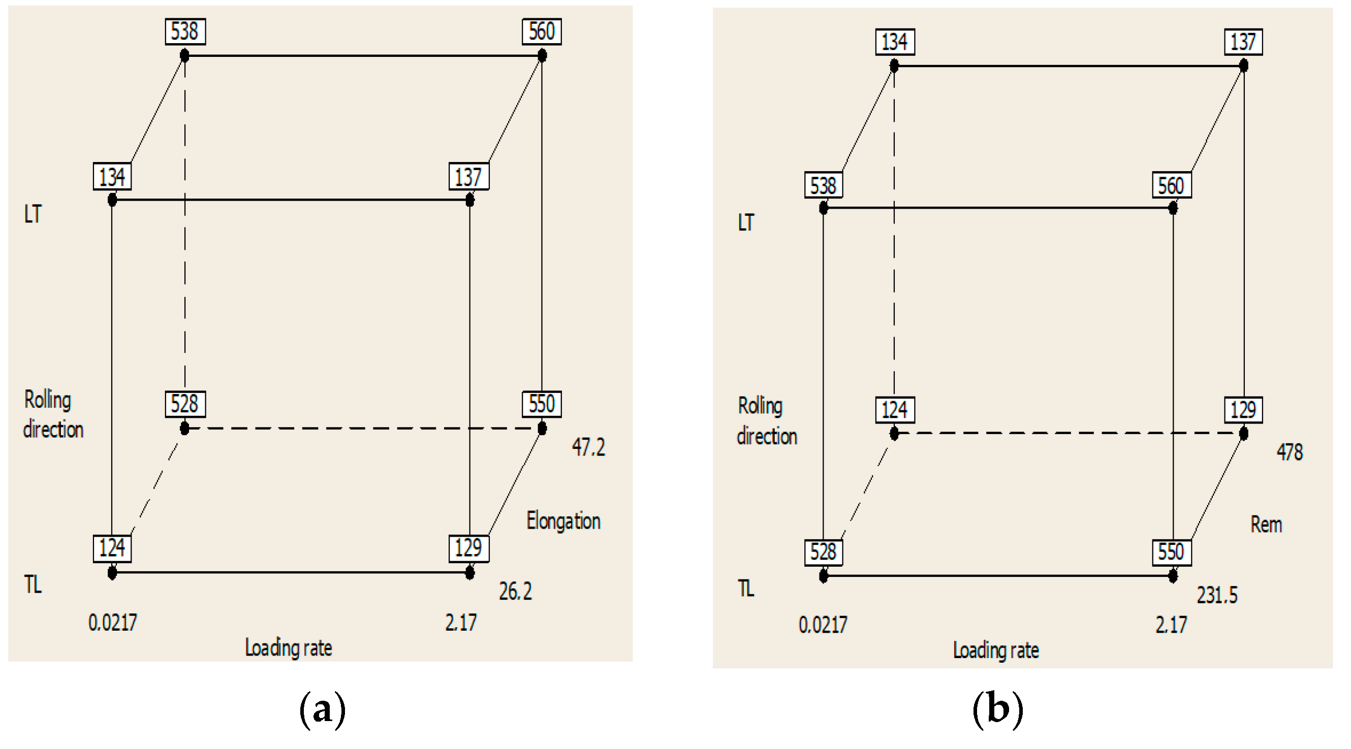
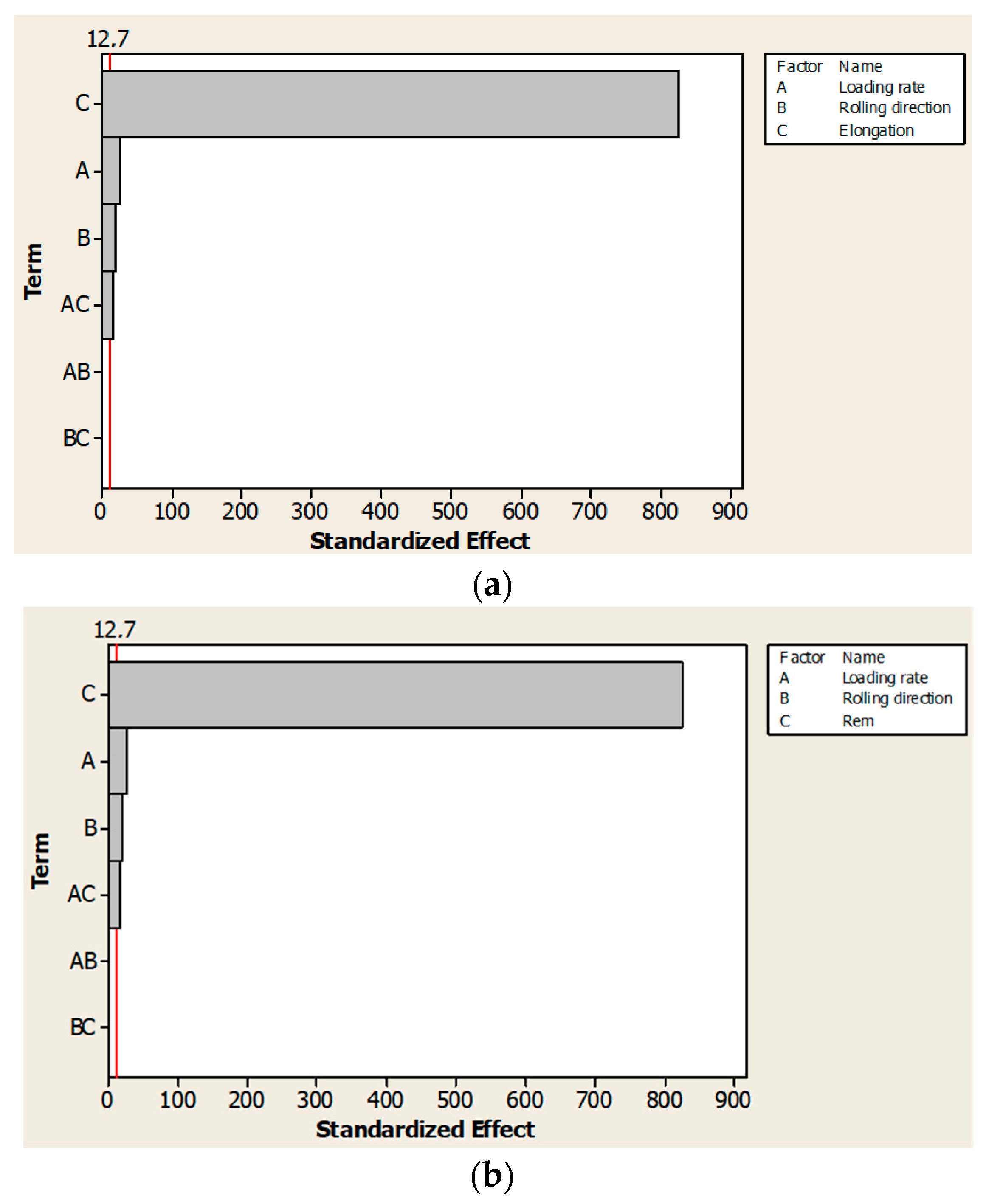
3. Results and Discussion
- XSG: T = 538
- DP: T = 124
- HR 45: T = 102.
4. Conclusions
Author Contributions
Funding
Data Availability Statement
Conflicts of Interest
References
- Fang, S.; Zheng, X.; Zheng, G.; Zhang, B.; Guo, B.; Yang, L. A new and direct R-value measurement method of sheet metal based on multi-camera DIC System. Metals 2021, 11, 1401. [Google Scholar] [CrossRef]
- Fang, X.-Y.; Gong, J.-E.; Huang, W.; Wu, J.-H.; Ding, J.-J. Novel characterisations of effective SIFs and fatigue crack propagation rate of welded rail steel using DIC. Metals 2023, 13, 227. [Google Scholar] [CrossRef]
- Parmadi, B.J.; Handika, N.; Sutanto, D.; Sentosa, B.O. Recycled aggregate concrete beam: Experimental study using Digital Image Correlation (DIC) and numerical study using multi-fibre Timoshenko beam element in CAST3M. In AIP Conference Proceedings; AIP Publishing: Damansara, Malaysia, 2023; Volume 2847. [Google Scholar]
- Ernawan, E.; Sjah, J.; Handika, N.; Astutiningsih, S.; Vincens, E. Mechanical properties of concrete containing ferronickel slag as fine aggregate substitute using Digital Image Correlation analysis. Buildings 2023, 13, 1463. [Google Scholar] [CrossRef]
- Bornert, M.; Brémand, F.; Doumalin, P.; Dupré, J.-C.; Fazzini, M.; Grédiac, M.; Hild, F.; Mistou, S.; Molimard, J.; Orteu, J.-J.; et al. Assessment of Digital Image Correlation measurement errors: Methodology and results. Exp. Mech. 2009, 49, 353–370. [Google Scholar] [CrossRef]
- Kharrat, F.; Khlif, M.; Hilliou, L.; Nouri, H.; Covas, J.A.; Bradai, C.; Haboussi, M. The application of 3D-Digital Image Correlation and analytical approaches on the bulge test for biaxial characterisation of biocomposite films. J. Braz. Soc. Mech. Sci. Eng. 2023, 45, 306. [Google Scholar] [CrossRef]
- Yang, R.; Li, Y.; Zeng, D.; Guo, P. Deep DIC: Deep learning-based Digital Image Correlation for end-to-end displacement and strain measurement. J. Mater. Proces. Tech. 2022, 302, 117474. [Google Scholar] [CrossRef]
- DIC. Available online: http://www.limess.com (accessed on 22 August 2022).
- Glushko, O. A simple and effective way to evaluate the accuracy of Digital Image Correlation combined with scanning electron microscopy (SEM-DIC). Results Mater. 2022, 14, 100276. [Google Scholar] [CrossRef]
- Musalamah, S.; Purnomo, H.; Handika, N. Method for determining fracture energy of a polypropylene coarse lightweight aggregate concrete beam using Digital Image Correlation. Eng. Proc. 2024, 63, 19. [Google Scholar] [CrossRef]
- Su, Y.; Rui, S.-S.; Han, Q.-N.; Shang, Z.-H.; Niu, L.-S.; Li, H.; Ishikawa, H.; Shi, H.-J. Estimation method of relative slip in fretting fatigue contact by Digital Image Correlation. Metals 2022, 12, 1124. [Google Scholar] [CrossRef]
- Del Rey Castillo, E.; Allen, T.; Henry, R.; Griffith, M.; Ingham, J. Digital Image Correlation (DIC) for measurement of strains and displacements in coarse, low volume-fraction FRP composites used in civil infrastructure. Compos. Struct. 2019, 212, 43–57. [Google Scholar] [CrossRef]
- Watrisse, B.; Chrysochoos, A.; Muracciole, J.-M.; Némoz-Gaillard, M. Analysis of strain localisation during tensile tests by Digital Image Correlation. Exp. Mech. 2001, 41, 29–39. [Google Scholar] [CrossRef]
- Eman, J.; Sundin, K.G.; Oldenburg, M. Spatially resolved observations of strain fields at necking and fracture of anisotropic hardened steel sheet material. Int. J. Solids Struct. 2009, 46, 2750–2756. [Google Scholar] [CrossRef]
- Dick, C.P.; Korkolis, Y.P. Mechanics and full-field deformation study of the ring hoop tension test. Int. J. Solids Struct. 2014, 51, 3042–3057. [Google Scholar] [CrossRef]
- Hlebova, S.; Ambrisko, L.; Pesek, L. Strain measurement in local volume by non-contact videoextensometric technique on ultra high strength steels. Key Eng. Mater. 2014, 586, 129–132. [Google Scholar]
- DIC. Available online: https://home.iitm.ac.in/kramesh/DIC.pdf (accessed on 20 August 2022).
- Vlk, M.; Florian, Z. Limit States and Reliabilit, 1st ed.; VÚT: Brno, Czech Republic, 2007; pp. 29–32. (In Czech) [Google Scholar]
- Trebuňa, F.; Šimčák, F. Resistance of Elements of Mechanical Systems, 1st ed.; Edícia vedeckej a odbornej literatúry TU: Košice, Slovakia, 2004; pp. 51–52. (In Slovak) [Google Scholar]
- Ambrisko, L.; Pesek, L. Determination the crack growth resistance of automotive steel sheets. Chem. Listy 2011, 105, 767–768. [Google Scholar]
- Ambrisko, L.; Cehlar, M.; Marasova, D. The rate of stable crack growth (SCG) in automotive steels sheets. Metalurgija 2017, 56, 396–398. [Google Scholar]
- Trebuňa, F.; Buršák, M. Limit States—Quarries, 1st ed.; Edícia vedeckej a odbornej literatúry TU: Košice, Slovakia, 2002; pp. 33–34. (In Slovak) [Google Scholar]
- Saxena, A. Nonlinear Fracture Mechanics for Engineers, 1st ed.; CRC Press: Boca Raton, FL, USA, 1998; pp. 154–156. [Google Scholar]
- Dhar, S.; Marie, S.; Chapuliot, S. Determination of critical fracture energy, Gfr, from crack tip stretch. Int. J. Press. Vessels Pip. 2008, 85, 313–321. [Google Scholar] [CrossRef]
- Brocks, W.; Anuschewski, P.; Scheider, I. Ductile tearing resistance of metal sheets. Eng. Fail. Anal. 2010, 17, 607–616. [Google Scholar] [CrossRef]
- Kumar, S.; Singh, I.V.; Mishra, B.K. A coupled finite element and element-free Galerkin approach for the simulation of stable crack growth in ductile materials. Theor. Appl. Fract. Mech. 2014, 70, 49–58. [Google Scholar] [CrossRef]
- Maiti, S.K.; Krishna Kishore, G.; Mourad, A.-H.I. Bilinear CTOD/CTOA scheme for characterisation of large range mode I and mixed mode stable crack growth through AISI 4340 steel. Nucl. Eng. Des. 2008, 238, 3175–3185. [Google Scholar] [CrossRef]
- Xu, W.; Ren, Y.; Xiao, S.; Liu, B. A finite crack growth energy release rate for elastic-plastic fracture. J. Mech. Phys. Solids 2023, 181, 105447. [Google Scholar] [CrossRef]
- Kovarik, O.; Cizek, J.; Klecka, J. Fatigue crack growth rate description of RF-plasma-sprayed refractory metals and alloys. Materials 2023, 16, 1713. [Google Scholar] [CrossRef]
- Jiang, J.; Falco, S.; Wang, S.; Giuliani, F.; Todd, R.I. Microcantilever investigation of slow crack growth and crack healing in aluminium oxide. Acta Mater. 2024, 119914, in press. [Google Scholar] [CrossRef]
- Pribulova, A.; Babic, J.; Baricova, D. Influence of Hadfield’s steel chemical composition on its mechanical properties. Chem. listy 2011, 105, 430–432. [Google Scholar]
- Ambrisko, L.; Pesek, L. The crack growth resistance of thin steel sheets under eccentric tension. Sadhana 2018, 43, 25. [Google Scholar] [CrossRef]
- STN 42 0347; Metal Testing, Fracture Toughness of Metals under Static Load. Slovak Technical Standard: Bratislava, Slovakia, 1990. (In Slovak)
- GOM; ARAMIS. User Manual—Software; GOM: Braunschweig, Germany, 2012. [Google Scholar]
- Ambrisko, L.; Pesek, L. The stretch zone of automotive steel sheets. Sadhana 2014, 39, 525–530. [Google Scholar] [CrossRef]
- Montgomery, D.C. Design and Analysis of Experiments, 10th ed.; J. Wiley: New York, NY, USA, 2020; pp. 97–99. [Google Scholar]


| Steel | Rp0.2 [MPa] | Rm [MPa] | A80 [%] | r | n | B [mm] | Bzc [µm] |
|---|---|---|---|---|---|---|---|
| XSG | 177 | 286 | 47.2 | 1.19 | 0.21 | 1.95 | 9.5 |
| HR 45 | 360 * | 449 | 27 | 0.87 | 0.14 | 1.80 | 12.3 |
| DP | 380 | 576 | 26.2 | 1 | 0.16 | 1.60 | 9.6 |
| Steel | Ffm [N] | Ffmin [N] | Fa [N] | N [103] | rc |
|---|---|---|---|---|---|
| XSG | 1920 | 480 | 720 | 60 | 0.25 |
| HR 45 | 3833 | 958 | 1437 | 30 | 0.25 |
| DP | 3132 | 783 | 1175 | 33 | 0.25 |
| Steel | Width before the Test [μm] | ρ before the Test [μm] | ρ before SCG [μm] |
|---|---|---|---|
| XSG | 1.3–2.6 | 0.65–1.3 | 780 |
| HR 45 | 1.3–2.6 | 0.65–1.3 | 490 |
| DP | 1.3–2.6 | 0.65–1.3 | 300 |
| Steel | L Deformation | T Deformation | ||
|---|---|---|---|---|
| Max. [%] | Mean [%] | Max. [%] | Mean [%] | |
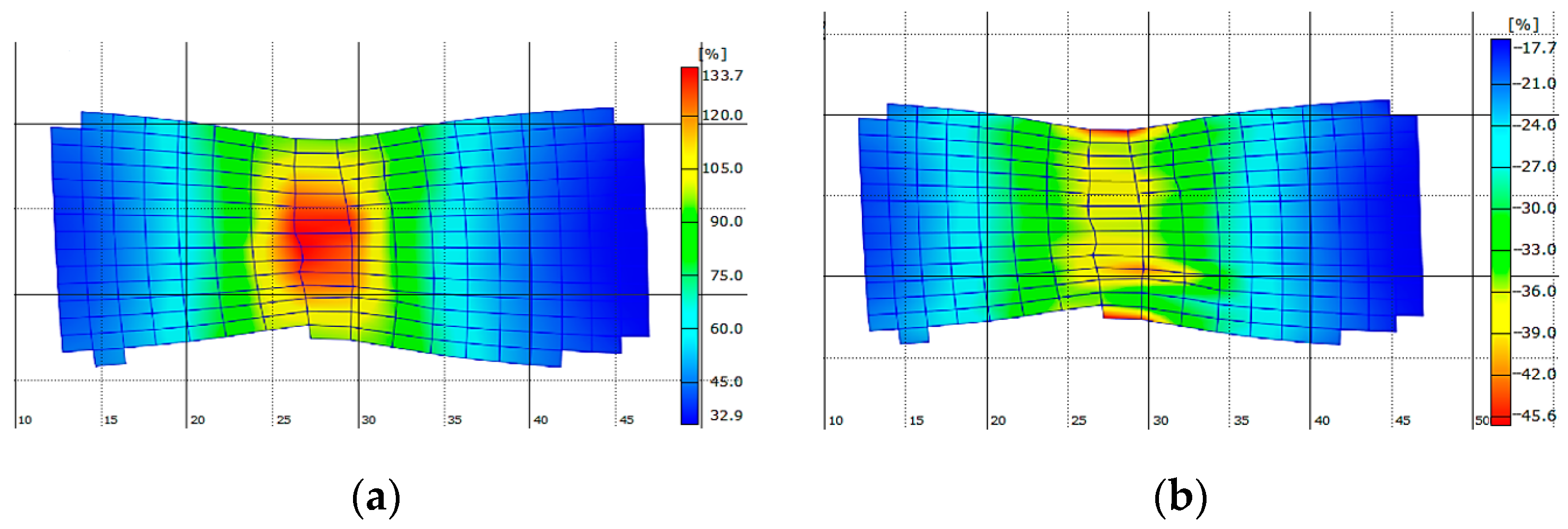
| XSG | 133.7 | 62.9 | 45.7 | 26.5 |
| HR 45 | 100.4 | 37.4 | 34.2 | 20.1 |
| DP | 81.2 | 33.8 | 23.5 | 14.5 |
| Run | Loading Rate [mm.s−1] | Specimen Orientation [–] | Elongation [%] or Rem [MPa] | T [–] | Steel |
|---|---|---|---|---|---|
| 1 | 0.0217 | TL | 26.2 or 478 | 124 | DP |
| 2 | 2.17 | TL | 26.2 or 478 | 129 | DP |
| 3 | 0.0217 | LT | 26.2 or 478 | 134 | DP |
| 4 | 2.17 | LT | 26.2 or 478 | 137 | DP |
| 5 | 0.0217 | TL | 47.2 or 231.5 | 528 | XSG |
| 6 | 2.17 | TL | 47.2 or 231.5 | 550 | XSG |
| 7 | 0.0217 | LT | 47.2 or 231.5 | 538 | XSG |
| 8 | 2.17 | LT | 47.2 or 231.5 | 560 | XSG |
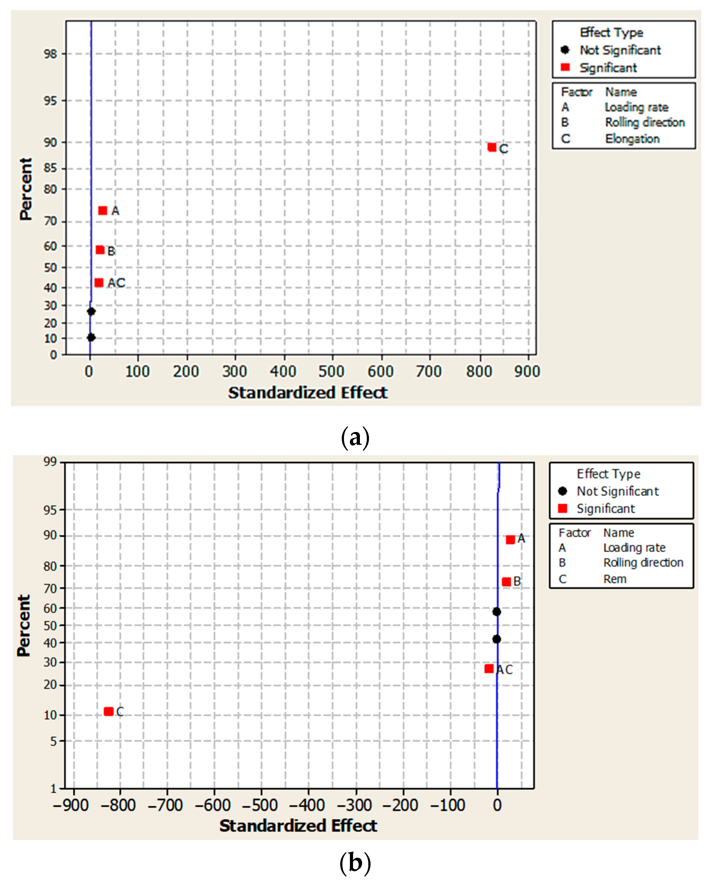
| Factors for Experiment 1 | Low Level | High Level | |
| A | Loading rate [mm.s−1] | 0.0217 | 2.17 |
| B | Specimen orientation [–] | TL | LT |
| C | Elongation A80 [%] | 26.2 | 47.2 |
| Factors for Experiment 2 | Low level | High level | |
| A | Loading rate [mm.s−1] | 0.0217 | 2.17 |
| B | Specimen orientation [–] | TL | LT |
| C | Rem [MPa] | 231.5 | 478 |
| Experiment 1 | A Loading Rate | B Specimen Orientation | C Elongation A80 |
| −1 (low level) | 331 | 333 | 131 |
| +1 (high level) | 344 | 342 | 544 |
| Effect of factors | 13.0 | 9.50 | 413 |
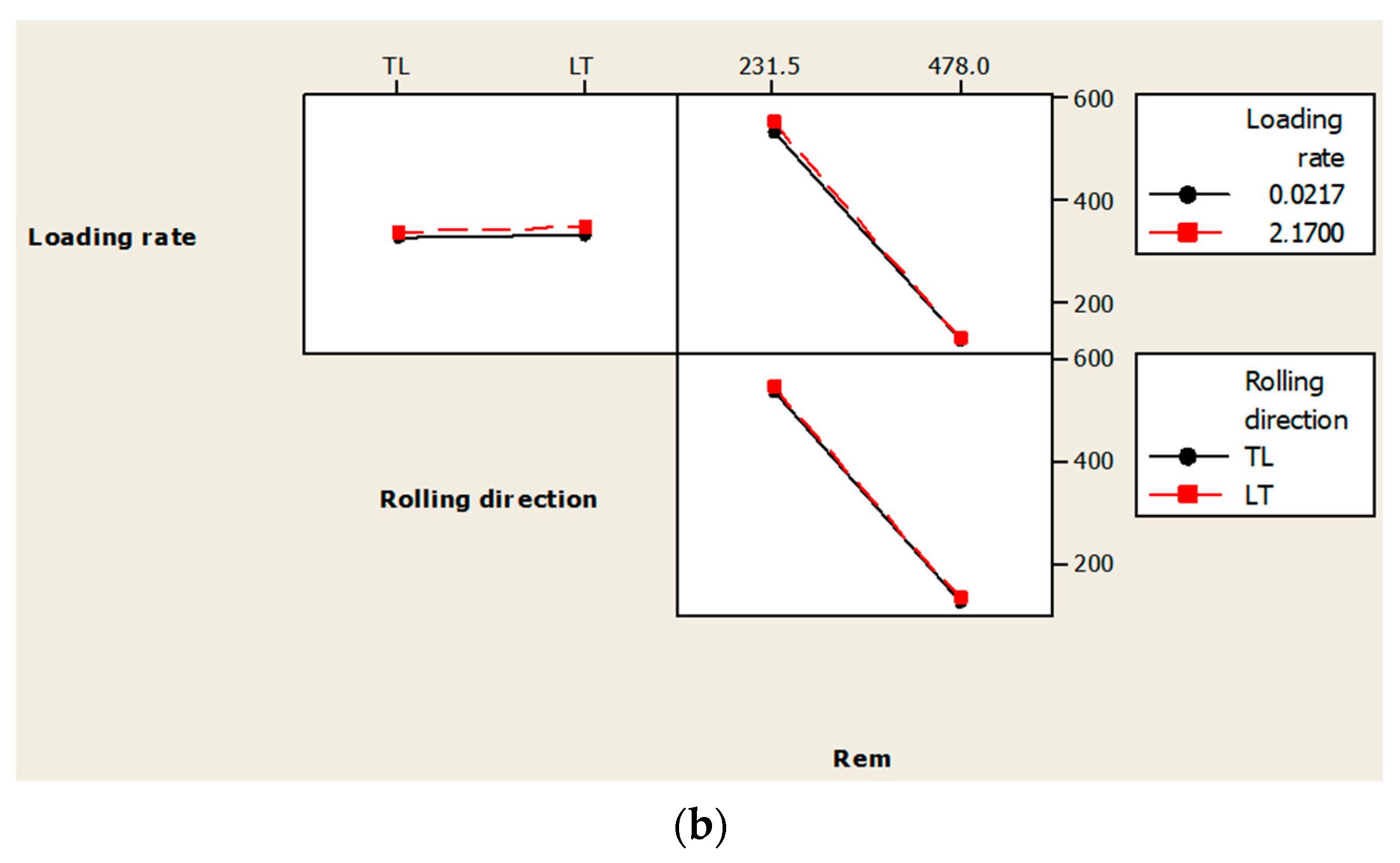
| Experiment 2 | A Loading rate | B Specimen Orientation | C Rem |
| −1 (low level) | 331 | 333 | 544 |
| +1 (high level) | 447 | 445 | 234 |
| Effect of factors | 116 | 113 | −310 |
| Experiment 1 | Coefficient | β0 | β1 | β2 | β3 | β12 | β13 | β23 |
| Value | 337.50 | 6.50 | 4.75 | 206.50 | −0.25 | 4.50 | 0.25 | |
| p-value | 0.000 | 0.024 | 0.033 | 0.001 | 0.500 | 0.035 | 0.500 | |
| Experiment 2 | Coefficient | β0 | β1 | β2 | β3 | β12 | β13 | β23 |
| Value | 337.50 | 6.50 | 4.8 | −206.5 | −0.20 | −4.50 | −0.20 | |
| p-value | 0.000 | 0.024 | 0.033 | 0.001 | 0.500 | 0.035 | 0.500 |
Disclaimer/Publisher’s Note: The statements, opinions and data contained in all publications are solely those of the individual author(s) and contributor(s) and not of MDPI and/or the editor(s). MDPI and/or the editor(s) disclaim responsibility for any injury to people or property resulting from any ideas, methods, instructions or products referred to in the content. |
© 2024 by the authors. Licensee MDPI, Basel, Switzerland. This article is an open access article distributed under the terms and conditions of the Creative Commons Attribution (CC BY) license (https://creativecommons.org/licenses/by/4.0/).
Share and Cite
Ambriško, Ľ.; Pešek, L. Non-Contact Evaluation of Deformation Characteristics on Automotive Steel Sheets. Metals 2024, 14, 566. https://doi.org/10.3390/met14050566
Ambriško Ľ, Pešek L. Non-Contact Evaluation of Deformation Characteristics on Automotive Steel Sheets. Metals. 2024; 14(5):566. https://doi.org/10.3390/met14050566
Chicago/Turabian StyleAmbriško, Ľubomír, and Ladislav Pešek. 2024. "Non-Contact Evaluation of Deformation Characteristics on Automotive Steel Sheets" Metals 14, no. 5: 566. https://doi.org/10.3390/met14050566
APA StyleAmbriško, Ľ., & Pešek, L. (2024). Non-Contact Evaluation of Deformation Characteristics on Automotive Steel Sheets. Metals, 14(5), 566. https://doi.org/10.3390/met14050566