Abstract
The axle bridge plays a crucial role in the bogie of low-floor light rail vehicles, impacting operational efficiency and fuel economy. To minimize the total cost of the structure and turning of axle bridges, an optimization model of structural and turning parameters was built, with the fatigue life, maximum stress, maximum deformation, and maximum main cutting force as constraints. Through orthogonal experiments and multivariate variance analysis, the key design variables which have a significant impact on optimization objectives and constraints (performance responses) were identified. Then the optimal Latin hypercube design and finite element simulation was used to build a Radial Basis Function (RBF) model to approximate the implicit relationship between design variables and performance responses. Finally, a multi-island genetic algorithm was applied to solve the integrated optimization model, resulting in an 8.457% and 1.1% reduction in total cost compared with the original parameters and parameters of sequential optimization, proving the effectiveness of the proposed method.
1. Introduction
Using a concave “U”-shaped axle bridge structure to connect two wheels with interference, 100% low-floor light rail vehicles can reduce the height of their floor surface from the ground [1]. The axle bridge is an important component of the vehicle bogie, and its—design structure is of great importance to improving the operating performance and fuel economy of light rail vehicles. Moreover, reasonable selection of the turning parameters of the axle bridge is an important way to ensure machining accuracy, improve production efficiency, and reduce production costs. Therefore, it is necessary to conduct structural and process parameter optimization for axle bridges.
Qu et al. [2] developed a multi-objective optimization model to reduce cutting force and surface roughness, and to improve the material removal rate, which was successfully solved by using the NSGA-II algorithm. Tian et al. [3] established a multi-objective optimization model aiming to minimize carbon emissions and processing time. In this case, the NSGA-II algorithm was used to obtain the optimal solution. With the spindle speed, feed per tooth, and transverse cutting depth as design variables, Yang et al. [4] formulated an optimization model targeted at minimizing carbon emissions and costs in milling, and used the genetic algorithm to obtain the optimal solution. Pourmostaghimi et al. [5] constructed a turning parameter optimization model with the material removal rate and processing cost as objectives, and surface roughness as the constraint. The particle swarm optimization algorithm was utilized to solve the model, yielding the optimal turning parameters. Qu et al. [6] investigated the effects of dry grinding, wet grinding, and nano-carbon fluid minimum lubrication on the grinding performance of ceramic matrix composites. They determined the optimal machining method through a controlled variable approach and orthogonal experiments, ultimately enhancing machining quality. Li et al. [7] developed a theoretical model for predicting grinding force in the grinding process, and optimized force parameters through a genetic algorithm.
In the process of optimization design, conventional methods often necessitate multiple iterations of finite element simulation analysis [8,9]. However, these methods involve high computational costs, which cannot meet the swift and efficient design requirements for engineering products. Consequently, surrogate models have emerged as a promising technology in the design field [10,11], extensively applied in complex equipment such as aircraft, ships, and automobiles [12]. Commonly employed surrogate models in engineering encompass the Polynomial Response Surface (PRS) [13], Radial Basis Function (RBF) [14], and Support Vector Regression (SVR) [15], among others. Wang et al. [16] established a multi-objective optimization model with the objectives of maximizing the machining efficiency and minimizing the tooth surface roughness. They utilized a regression model to approximate the implicit relationship between grinding parameters and tooth surface roughness, and employed the particle swarm optimization algorithm for the optimization solution. Wang et al. [17] constructed the response surface model to optimize the front collector structure using different materials. The feasibility of the response surface model was validated through metrics R2 and RMSE, and the MIGA algorithm was employed for seeking the optimal solution. Gao et al. [18] employed the Kriging model and a genetic algorithm to optimize welding process parameters, resulting in the optimal weld geometry shape. Wang et al. [19] integrated sensitivity analysis with structural contribution analysis to identify design variables for the lightweight body frame of an electric bus. Subsequently, RBF and NSGA-II were utilized to fit and solve the collaborative optimization model. Li et al. [20] assessed the fitting accuracy of RBF, PRS, SVR, and Kriging models through cross-validation error. RBF, exhibiting the highest accuracy, was employed to approximate the implicit relationship between EDM parameters and the performance response of 304 steel. Finally, NSGA-II was used for multi-objective optimization. Gao et al. [21] focused on the welding frame of the bogie, establishing the lightweight design model with static strength and welding fatigue as constraints. The Kriging model and an adaptive sequential approximation optimization method were then applied for the solution.
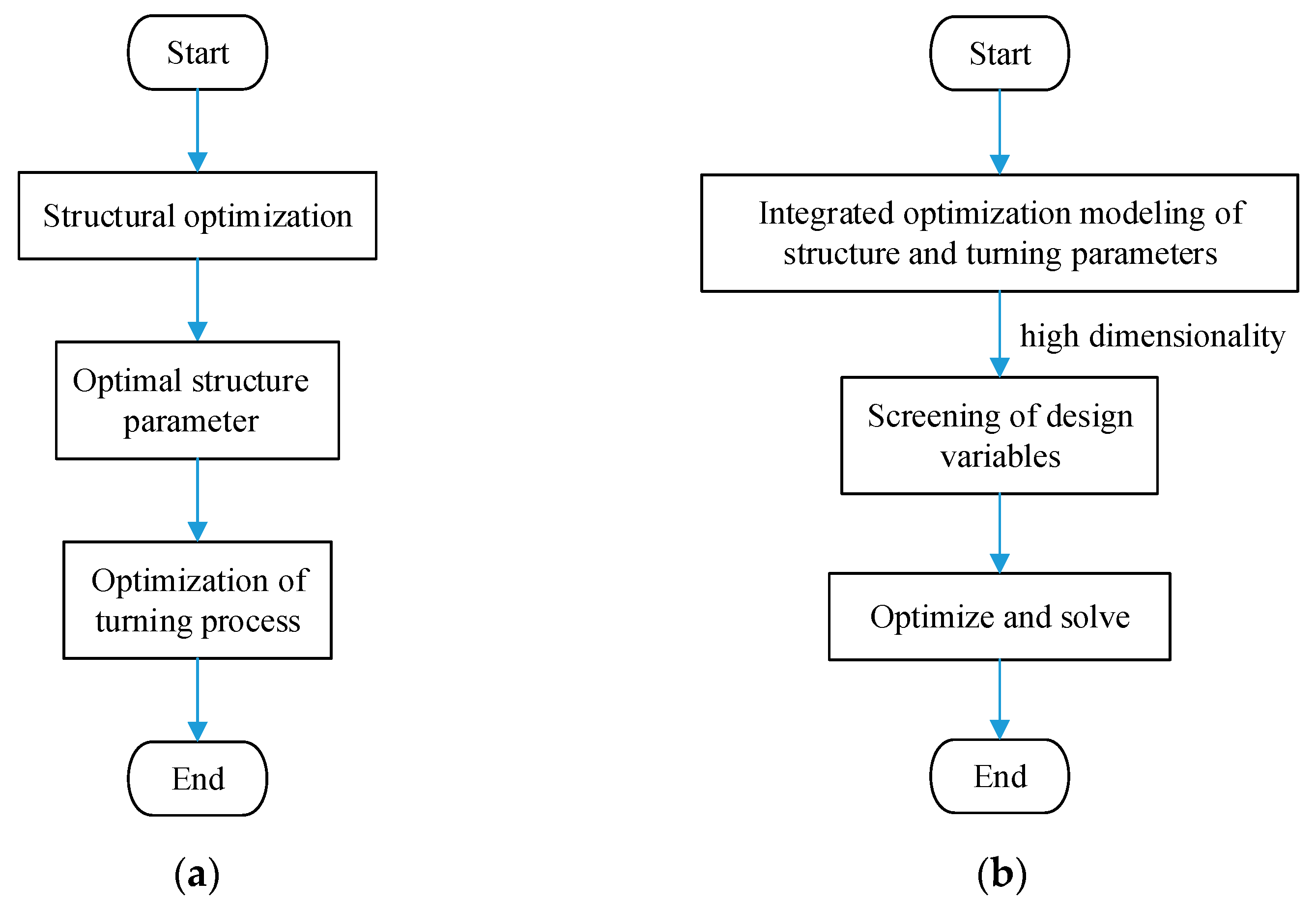
In existing cost-driven optimization research focusing on both structural and process parameters, the majority of researchers employ a sequential optimization approach (as illustrated in Figure 1a), leading to a separation between structural and process design, and making it challenging to minimize the total cost of both. Moreover, during the optimization process, the results of a performance response analysis (finite element simulations or physical experiments) are often directly utilized, resulting in high optimization costs. Therefore, this paper proposes an integrated optimization method for the axle bridge structure and process of low-floor light rail vehicles. It establishes an optimization model with the axle bridge structural parameters and process parameters as variables, and cost as the objective. Additionally, it introduces an RBF model to replace the implicit relationship between the axle bridge structure, process parameters, and performance response. Finally, the optimized model is solved using a multi-island genetic algorithm to obtain the optimal combination of axle bridge structure and process parameters. The innovation lies in the integration of optimization models, which reduces overall costs compared to previous methods, where structural and parameter optimizations were conducted sequentially, as depicted in Figure 1b.
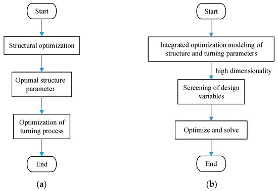
Figure 1.
Comparison of sequential and integrated optimization of structural and turning parameters: (a) flowchart of sequential optimization; (b) flowchart of integrated optimization.
2. Optimization of Structural Parameters
As an important component of the bogies of low-floor light rail vehicles, the optimization design of the axle bridge is of great importance for improving the operating performance and fuel economy of light rail vehicles [22]. Low-floor light rail vehicles adopt concave “U”-shaped axle bridges to reduce the height from the floor to the ground [1]. The axle bridge structure used in this paper, which consists of the axle journal, axle head, axle body, and primary spring seat, is shown in Figure 2. In the actual working process of an axle bridge, stress is a critical factor affecting its strength, because excessive stress can lead to axle bridge failure. Deformation is a key factor affecting the stiffness of the axle bridge. Excessive deformation not only affects passenger comfort but also poses safety concerns. Fatigue life is crucial for the long-term safe working of an axle bridge. Therefore, the stress, deformation, and fatigue life are used as the constraints in the structural optimization of an axle bridge.
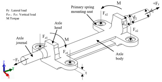
Figure 2.
Schematic diagram of axle bridge structure.
2.1. Finite Element Simulation
Based on the TB/T 3549.1-2019 [23] standard, the analysis and calculation of the magnitude of loads on an axle bridge were determined according to Formulas (1)–(3). The technical parameters utilized for these calculations are detailed in Table 1.

Table 1.
Main technical parameters of low-floor light rail vehicles.
To ensure safe operation under extreme working conditions, the applied load of an axle bridge under the combined action of vertical, lateral, and torsional loads was comprehensively analyzed and calculated.
The vertical load is
where (N) is the vertical load applied on the left side of the axle bridge; (N) is the vertical load applied on the right side of the axle bridge; and nb is the number of bogies (take as 2 for two bogies per carriage).
The lateral load is
where, Fy (N) is the magnitude of the lateral load applying to each bogie.
Moreover, to simulate the distortion of the bogie under curved track conditions, a torque was applied at the spring seat of the axle bridge. The formulation of torque is
Based on the Formulations (1)–(3), the vertical, lateral, and torque loads were 16,892.82 N, 21,689.91 N, and 3939.94 N·m, respectively. The axle bridge material used was 25CrMo low-carbon alloy steel (Trading Company, Liaocheng, China), and its main mechanical parameters [24] are shown in Table 2.
Table 2.
Mechanical parameters of 25CrMo.
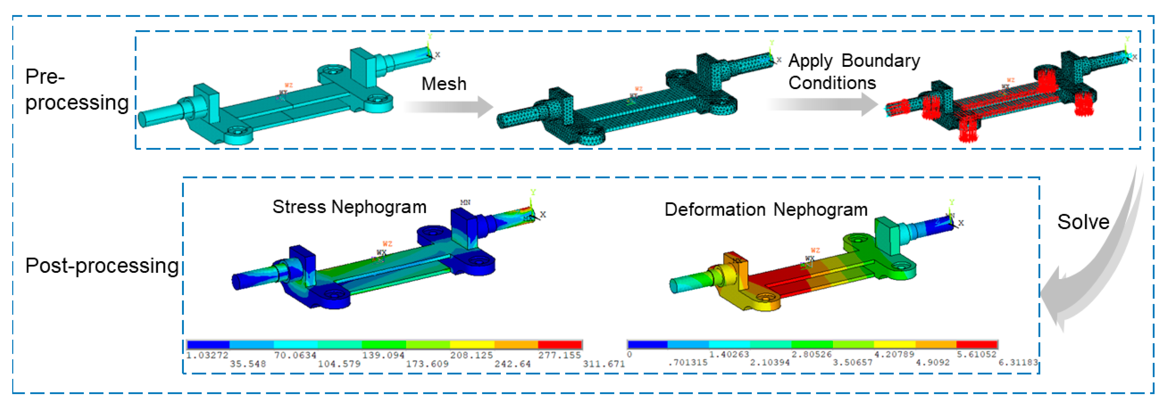
The 3D model of the axle bridge was drawn and simplified using SolidWorks, and meshed using ANSYS in a tetrahedral manner. The results are shown in Figure 3. The number of cells in the model was 112,977, and the number of nodes was 200,053.
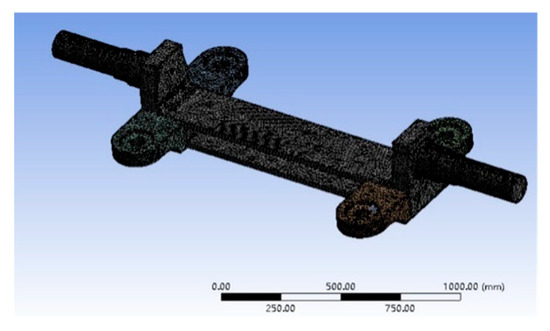
Figure 3.
Axle bridge finite element mesh model.
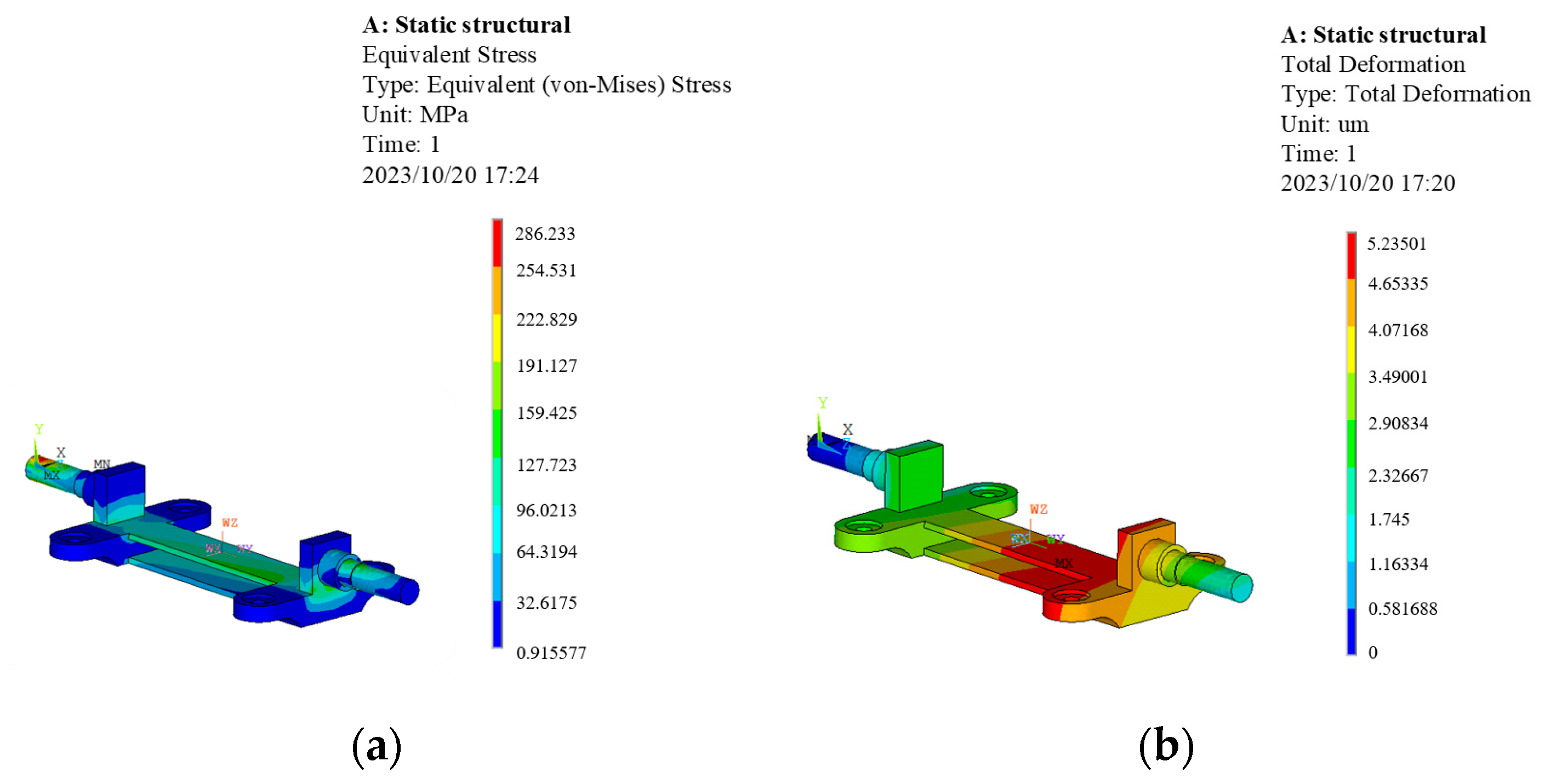
The vertical load and torsional load were applied to the primary spring seat, and the lateral load was applied to the axle journal. The constraints were applied to the axle journal at both ends. The maximum stress and deformation nephogram were obtained through static analysis, as shown in Figure 4. The maximum stress was 286.233 MPa, and the maximum deformation was 5.23501 × 10⁻³ mm.
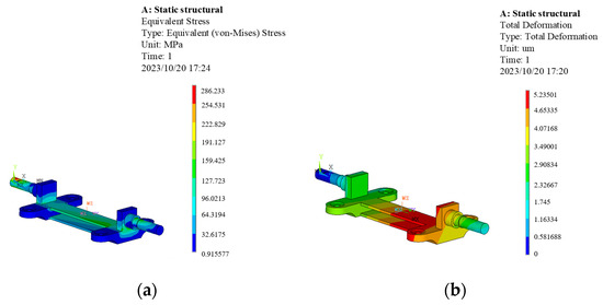
Figure 4.
Nephograms of maximum stress and maximum deformation: (a) stress nephogram; (b) deformation nephogram.
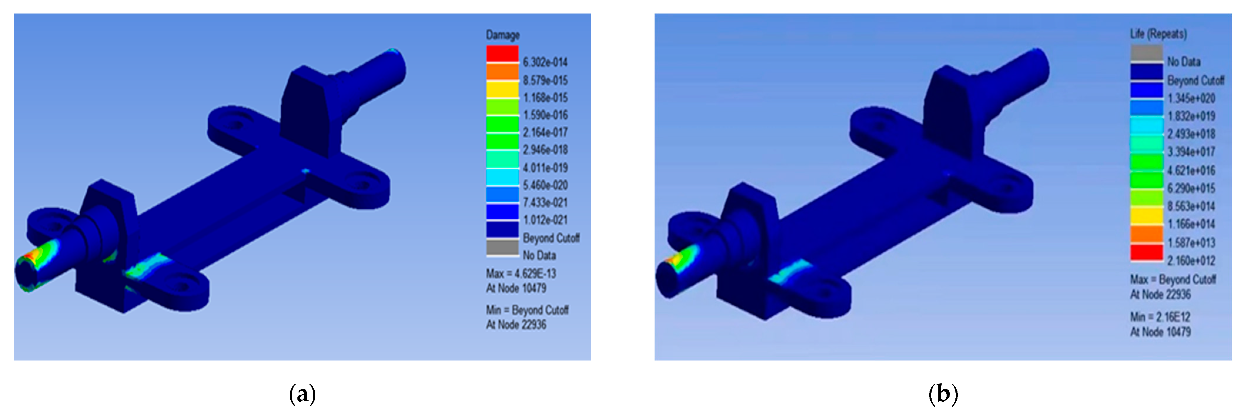
Based on the statics analysis results, the fatigue life analysis of the axle bridge was carried out. The fatigue damage and life nephograms were obtained, as shown in Figure 5. From the damage nephogram, the damage degree of each part of the axle bridge can be seen. The red is the weak area, which is located at the left end of the axle journal and near the arc of the connection between the axle journal and the axle head. This indicates that these areas are prone to fatigue failure, which is basically consistent with the results of the static strength analysis.

Figure 5.
Fatigue life analysis of axle bridge: (a) fatigue damage nephogram; (b) fatigue life nephogram.
According to the analysis results, the minimum life of the axle bridge was occurrences at the 10,479 node, which is far greater than the requirements of the enterprise. From the results of the statics and fatigue analysis of the axle bridge, the stress, deformation, and life of the axle bridge are surplus, thus there is still space for lightweight design.
2.2. Parametric Modeling
To reduce the finite element simulation time, it was necessary to conduct parametric modelling by means of APDL. Parametric modelling can achieve rapid adjustment of size parameters, automatic imposing of load and constraints, automatic generation of finite element analysis models, and rapid acquisition of response values such as stress, deformation, and fatigue life. The parametric modelling process of the axle bridge is shown in Figure 6.

Figure 6.
Parametric modeling process of axle bridge.
2.3. Structural Optimization
To reduce the blank costs, the optimization model of the axle bridge was built in Equation (4), which takes the diameter of the axle journal , and the thickness of the primary spring seat as design variables, and takes the stress, deformation, and fatigue life as constraints.
where is the design variable; is the cost of the axle bridge blank, which can be calculated using the product of weight and unit price; L is the fatigue life; is the maximum deformation; and is the maximum stress.
The value range and initial value of the structural parameter of the axle bridge are shown in Table 3.
Table 3.
Design variables and value range in structural optimization.
A full factorial design (FFD) with 4-factor and 3-level was conducted, and 64 groups of structural parameters were randomly selected from the FFD samples. APDL was then performed for parametric modeling to obtain the stress, deformation, and fatigue life values at the 64 groups of structural parameters. Partial sample points and performance response values are shown in Table 4.
Table 4.
Partial sample points for structural optimization of axle bridge.
Based on the 64 groups of structural parameters and corresponding simulation results, an RBF model was built to fit the implicit relationship between design variables and responses. Then multi-island genetic algorithm was used to solve the structural optimization model. The parameters of multi-island genetic algorithm were iterations of 2000, islands number and population size of 10, and probability of crossover and variation of 0.01. The comparison of the axle bridge structural parameters before and after optimization is shown in Table 5.
Table 5.
Comparison of axle bridge structural parameters before and after optimization.
The structural parameters after optimization were imported into the parametric model for statics analysis and fatigue life analysis. The maximum stress was 313.408 MPa, the maximum deformation was 6.395 × 10⁻³ mm, and the minimum life was 1.029 × 10⁹ times. Therefore, under the premise that the stress, deformation, and service life meet the constraints, the weight of the optimized axle bridge was reduced by 37.836 kg and the weight reduction rate was 8.05%. Multiplied by the unit price, the total cost of the axle bridge blank was reduced by $47.56 after structural optimization.
3. Optimization of Turning Parameters
In turning, the reasonable selection of cutting parameters is an important way to ensure machining accuracy, improve production efficiency, and reduce production costs. Cutting force is an important factor influencing machining quality; excessive cutting force can cause vibration in the machining system, thereby affecting machining accuracy. Therefore, using the optimal structural parameter in Section 2, the optimization model for the axle bridge turning parameters was built with turning cost as the objective and cutting force as the constraint.
3.1. Optimization Model of Turning Parameters
In practice, multi-pass turning is used to machine the axle journal. The turning parameter optimization model was built with turning cost as the objective, and the cutting speed, feed rate, and depth of cut in the rough machining, semi precision machining, and precision machining stages as variables, as shown in Equation (5). The design variables and value range are shown in Table 6.
where [25] is the turning cost, is the main cutting force, and is the maximum allowable value of . According to the literature [26], is calculated as follows:
where is the actual processing cost; is the cost of workpiece installation and disassembly, as well as the cost of machine idle; is the tool replacement cost; and is the tool cost. is the unit time cost; is the cutting time; is the workpiece installation and disassembly time; is the machine idle time; is the tool replacement time; is the cost of per blade of the tool; and is the tool life. Formula (4) is used to calculate .
where , , and are the length of different segments of the axle journal; and are the diameters of axle journal (in Figure 2); and is the blank allowance.
Table 6.
Design variables and value range in optimization of turning parameters.
The parameters and values involved in Equations (6) and (7) are shown in Table 7.
Table 7.
Parameter value of turning parameter optimization model of axle bridge.
3.2. AdvantEdge Turning Simulation
To obtain the cutting force at different turning parameters, AdvantEdge turning simulation was conducted in this paper. The AdvantEdge turning simulation process includes preprocessing the simulation parameter setting; solving; and result postprocessing; as shown in Figure 7. The simulation parameters for AdvantEdge turning are shown in Table 8. According to the cutting theory, the ratio of main cutting force, back force, and feed force in cutting is about 1:0.4:0.25 [27]. Among the cutting forces, the main cutting force is the largest, followed by the back force, and the feed force is the smallest. Therefore, the main cutting force is generally used as the response index during the cutting process.
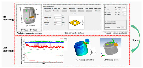
Figure 7.
Process of AdvantEdge simulation.
Table 8.
Parameter value of AdvantEdge turning.
In this paper, YT15 cemented carbide was used as the cutting tool material. The mechanical properties of YT15 is as follows: strong hardness (91 HRA), bending strength (1180 MPa), and high density (12 g/cm3). Moreover, YT15 exhibits a high bonding temperature and robust oxidation resistance. Therefore, YT15 was used in this paper to turn the axle bridge.
To reduce the optimization cost of the turning parameters, RBF was used to fit the implicit relationship between the turning parameters and the main cutting force. In this paper, an 8-factor and 4-level orthogonal experiment was designed to perform an AdvantEdge turning simulation to obtain the main cutting force. The main cutting force (N) for rough machining; (N) for semi precision machining; (N) for precision machining; and the turning cost f(x) ($), are shown in Table 9.
Table 9.
Sample points of orthogonal experiment in optimization of turning parameters.
3.3. Optimization Solution
The multi-island genetic algorithm was used to solve the optimization model of axle bridge turning parameters, and optimal turning parameters were obtained. The comparison of turning parameters before and after optimization is shown in Table 10.
Table 10.
Comparison of turning parameters before and after optimization.
Based on the spindle speed, feed rate, and depth of cut after optimization, an AdvantEdge turning simulation and cost calculation were conducted. The main cutting forces for precision machining, semi precision machining, and rough machining were 539.56 N, 2340.98 N, and 4460.17 N, respectively, all of which met the constraint conditions. After optimization, the turning cost was $110.63, which is $4.99 less than that before optimization, with a decrease of 4.316%.
4. Integrated Optimization of Structural and Turning Parameters
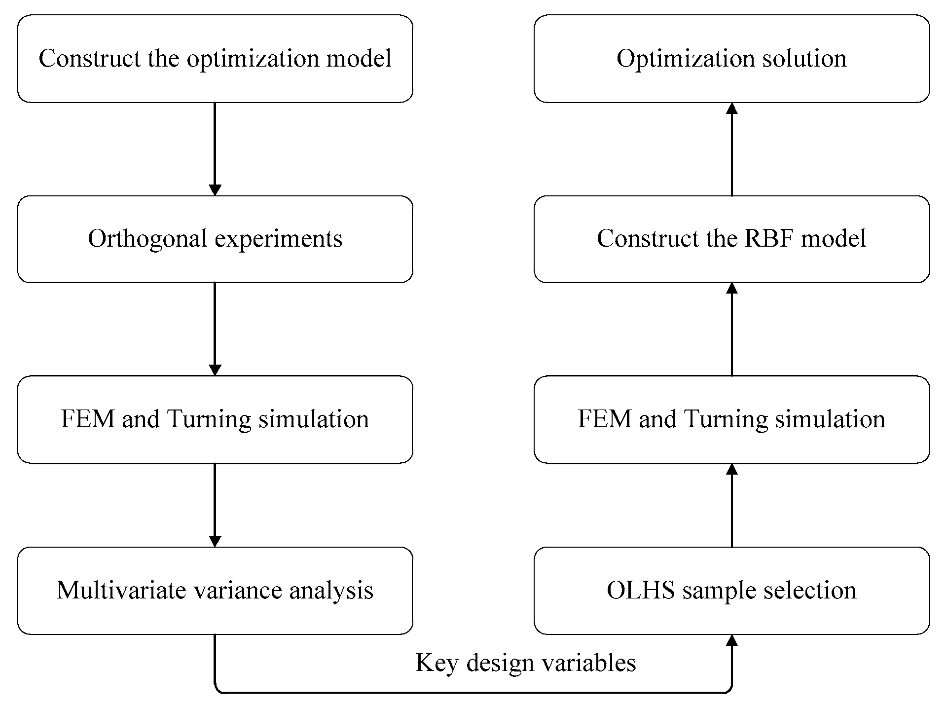
In order to further reduce the cost of the structural and turning parameters, the integrated optimization method was developed in this paper. Orthogonal experiments and multivariate variance analysis were used to reduce the dimension of optimization problems and improve the optimization efficiency. Through orthogonal experimental design, and utilizing ANSYS and AdvantEdge for finite element and turning simulations, samples and corresponding performance response values were obtained. Subsequently, multivariate variance analysis was employed to screen design variables, selecting those significantly impacting the objective and performance responses as optimization variables. Utilizing the selected design variables, optimal Latin hypercube sampling was employed to acquire sample points, and response values were obtained through simulation. Based on the OLHS samples and corresponding performance responses, the RBF model was constructed to fit the implicit relationship between design variables and responses. Finally, an integrated optimization model was established with total cost as the optimization objective, incorporating axle bridge structural parameters and turning process parameters as variables. The specific process is illustrated in Figure 8.
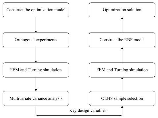
Figure 8.
Design of experiments and optimization process.
4.1. Radial Basis Function
Radial Basis Function (RBF) is a typical three-layer (input layer, hidden layer, output layer) feedforward neural network [28], which is characterized by strong nonlinear approximation capability, efficiency, simplicity, and adaptability [29]. Therefore, RBF was chosen in this study to approximate the implicit relationship between variables and responses. During the optimization process, using the RBF model instead of the finite element simulation and turning simulation can significantly reduce the optimization cost. Furthermore, utilizing the accurate RBF approximation of the variable-response implicit relationship enables the selection of more precise optimization algorithms, consequently improving optimization accuracy.
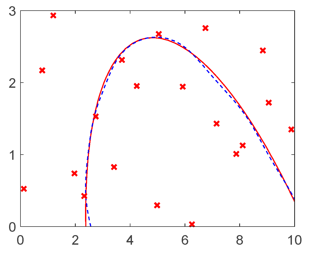
To verify the effectiveness of RBF, the nonlinear numerical example used was as follows [30]:
Twenty samples obtained via Latin hypercube sampling were selected to construct the RBF model. The samples (red cross), true curve of (red solid line), and predicted curve using RBF (blue dashed line) are shown in Figure 9. As can be seen, the RBF model has good fitting ability to the nonlinear example with fewer samples. Therefore, RBF was used in this paper to approximate the implicit relationship between optimization variables and performance responses.
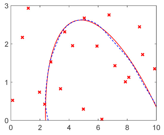
Figure 9.
Numerical example.
4.2. Multivariate Variance Analysis
The design parameters for integrated optimization include structural parameters (); rough turning process parameters (); semi precision turning process parameters (); and precision turning process parameters (). To reduce the cost of integrated optimization, orthogonal experiments and multivariate variance analysis were used to screen design variables that have a great influence on the performance responses. In this section, orthogonal experiments with 12-factor and 4-level were used for experimental design (as shown in Table 11). Finite element analysis and turning simulation experiments were then carried out for each group of sample points. The performance response values such as weight; stress; deformation; life; rough machining main cutting force ; semi precision machining main cutting force ; and precision machining main cutting force were obtained, as shown in Table 12.
Table 11.
Table of factor level for orthogonal experiments.
Table 12.
Sample points of orthogonal experiment in integrated optimization.
Based on the sample points of orthogonal experiments, multivariate variance analysis was conducted on the design variables and performance responses. The detailed process of multivariate variance analysis can be found in [31]. The analysis results are shown in Table 13, where p < 0.05 indicates that the design variable has great influence, and p < 0.01 indicates that the design variable has even greater influence.
Table 13.
Results of Multivariate Variance Analysis.
According to the results of the multivariate variance analysis (as shown in Table 11), were regarded as having affected the weight and deformation significantly, and were regarded as having affected the maximum stress significantly, and were regarded as having affected the main cutting force and turning cost significantly. Therefore, six optimization variables were selected based on their significant influence on the objective and response values: structural parameters of the axle bridge, as well as feed rate and cutting depth in the turning process.
4.3. Integrated Optimization Model
To reduce the total cost of the blank and the turning process of an axle bridge, a mathematical model for integrated optimization was built with total cost as the objective, and the dimensions and turning process parameters of the axle bridge structure as design variables, as shown in Equation (9).
where and , respectively, represent the cost of the blank and the turning process of an axle bridge; represents the minimum allowable life of the axle bridge; , and , respectively, represent the maximum stress, maximum deformation, and maximum main cutting force of the axle bridge during FEM and turning simulation; and , , and are the maximum allowable values for the corresponding performance responses.
4.4. Optimal Latin Hypercube Sampling
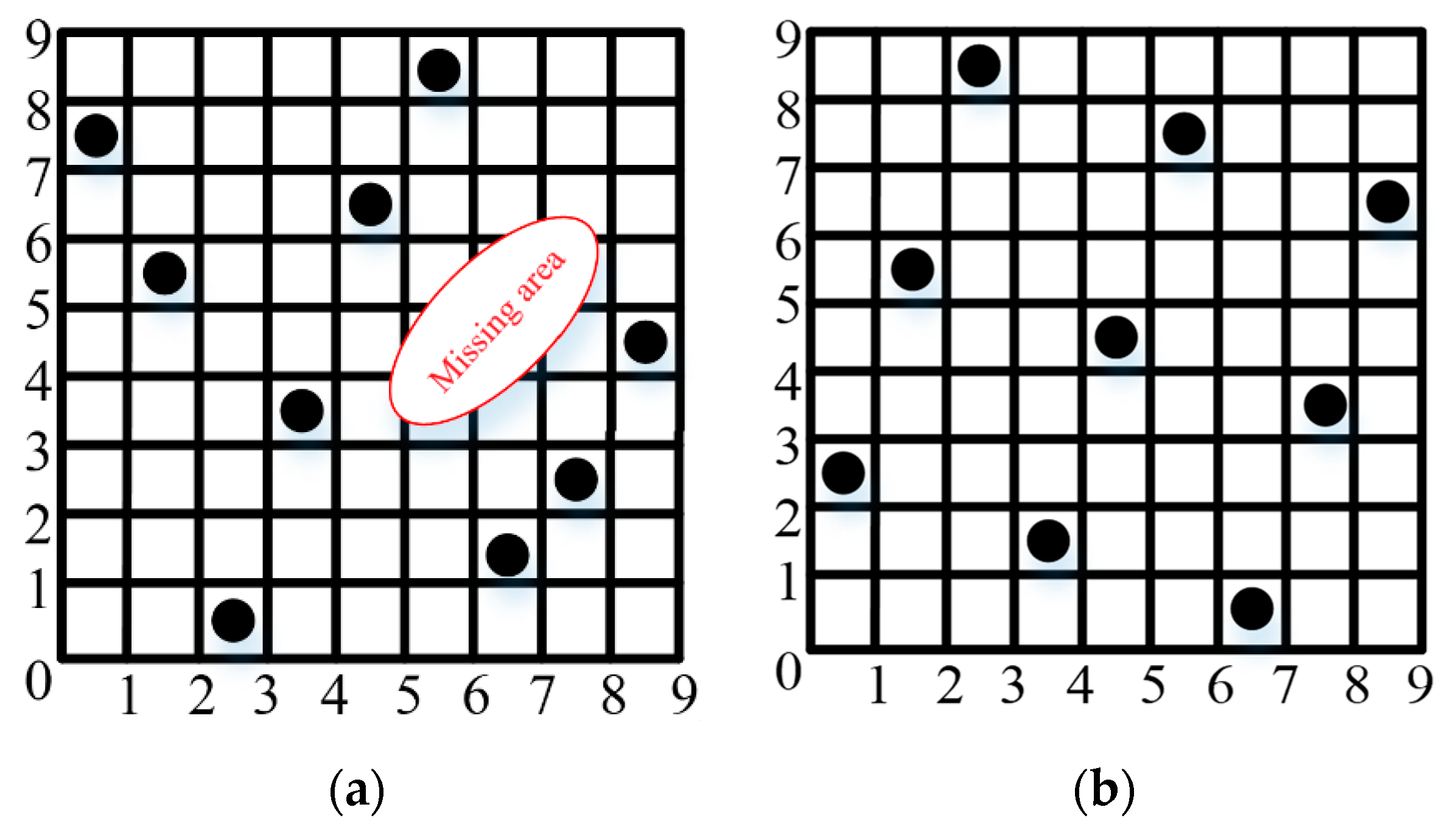
Based on the screened design variables, the design of the experiments was reconducted. Compared with traditional sampling methods, Latin Hypercube Sampling (LHS) has a more uniform filling performance in the design domain. However, some sample points in LHS cannot be evenly selected in the design domain, so the fitting accuracy of the surrogate model may be biased. Optimal Latin Hypercube Sampling (OLHS) improves LHS by increasing the distance between sample points. It distributes all sample points as evenly as possible within the design domain, which can show better uniformity and space filling. It can thus fit the relationship between variables and responses more accurately and truly.
As can be seen from Figure 10a, sample points in some areas of LHS are too concentrated, and samples in other areas are missed. By contrast, sample points in OLHS are more even and there is no missing area, as shown in Figure 10b.
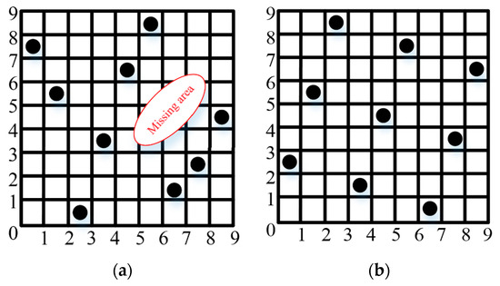
Figure 10.
Comparison of LHS and OLHS: (a) Latin hypercube Sampling; (b) optimal Latin hypercube sampling.
Based on the results of multivariate variance analysis, 60 samples were selected via the OLHS method. Statics and turning simulation analysis were conducted to obtain the weight, stress, deformation, life, and main cutting force at these sample points. Partial sample points are shown in Table 14.
Table 14.
Partial sample points of optimal Latin hypercube sampling.
4.5. Integrated Optimization Process
In order to keep the axle bridge strength and cutting force within the allowable range, and minimize the total cost of structure and turning processes, the RBF model and multi-island genetic algorithm were introduced in the integrated optimization of the axle bridge. The integrated optimization process is shown in Figure 11.
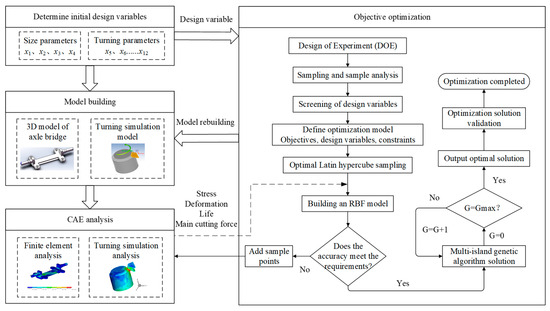
Figure 11.
Integrated optimization process of axle bridge structure and turning processes.
Step 1: Determine the initial design variables and value range. In this paper, the existing structural and turning parameters were used as the initial design variables, whose ranges were determined according to the requirements of the enterprise.
Step 2: Screening of design variables. Firstly, 49 groups of sample points were obtained via 12-factor and 4-level orthogonal experiments. The performance responses of each group of sample points were obtained using ANSYS statics and AdvantEdge turning simulation analysis. Then, multivariate variance analysis was conducted to select the design variables which have great impact on weight, stress, deformation, and the main cutting force.
Step 3: Optimal Latin hypercube sampling and RBF modeling. Based on the screened design variables in Step 2, 60 groups of sample points were selected using the OLHS method, and simulation analysis was carried out. On this basis, the RBF surrogate model was built to fit the implicit relationship between the design variables and performance responses.
Step 4: Optimization solution and result validation. The multi-island genetic algorithm was used to optimize the surrogate model, and the results were verified.
4.6. Optimization Solution
In the integrated optimization process of the axle bridge structure and process, the initial design variables consisted of the structural parameters of the axle bridge, and machining parameters including roughing, semi-finishing, and finishing cutting, denoted as to . Through multivariate variance analysis on these initial design variables, key variables significantly impacting the performance responses were identified, including the axle bridge dimension parameters , the feed rate in the finishing process , and the turning depth . The reduction in dimension parameters after optimization achieved a structural weight reduction, thereby lowering the raw material cost of the axle bridge. Additionally, the reduction in turning parameters led to a decrease in machining costs, resulting in reduced overall cost.
The integrated optimization model of the axle bridge was solved via multi-island genetic algorithm. The comparison of design variables before and after optimization is shown in Table 15 and Table 16.
Table 15.
Comparison of design variables before and after optimization.
Table 16.
Performance before and after optimization, and comparison between predicted and true values.
As can be seen from Table 16, compared with the initial value, the total cost after sequential optimization was reduced by 7.439%, from $706.392 to $653.843. Furthermore, the total cost of integrated optimization is $646.65, which is 1.1% lower than that of sequential optimization.
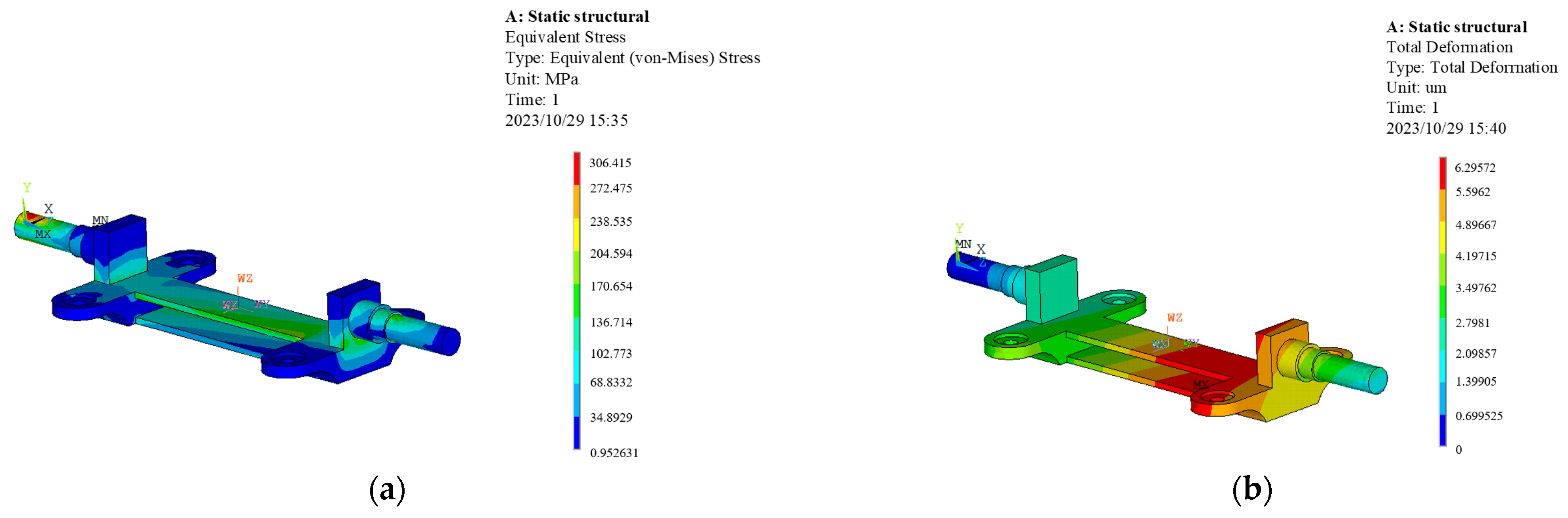
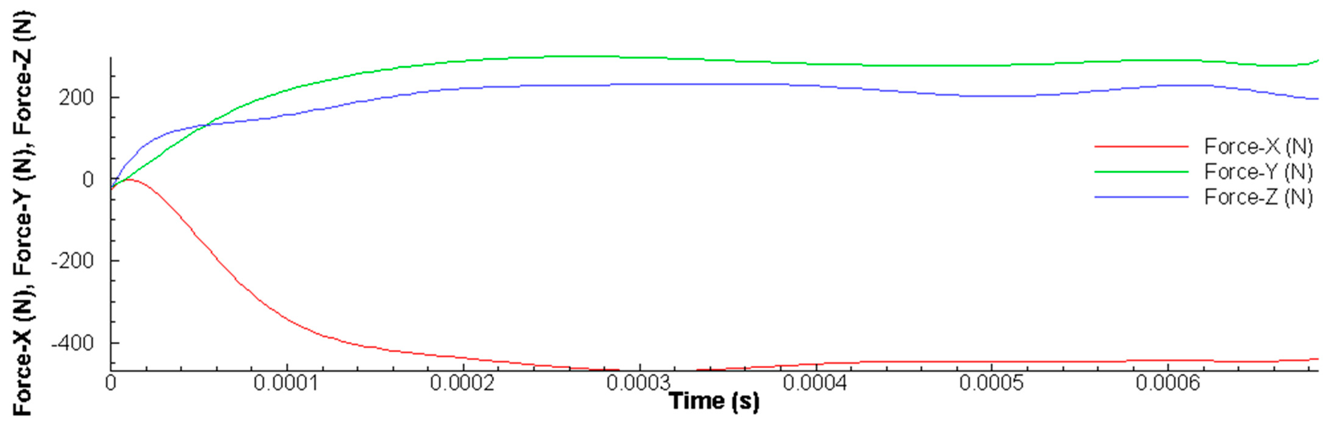
Based on the design variables after optimization, the 3D model and turning model of the axle bridge were rebuilt. After simulation, the stress, deformation, and precision machining cutting force were obtained, as shown in Figure 12 and Figure 13, which are all within the allowable range.
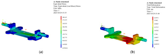
Figure 12.
Nephogram of maximum stress and deformation: (a) maximum stress nephogram; (b) maximum deformation nephogram.
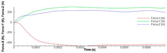
Figure 13.
Curve of cutting force for precision machining.
5. Conclusions
In this paper, an integrated optimization approach for both axle bridge structure and turning processes based on RBF was proposed.
- (1)
- The optimization of the structural parameters of the axle bridge was conducted. A full factorial experiment with 4-factor and 3-level was designed, from which 64 groups of sample points were randomly selected, and the parametric model was used for simulation. Based on the simulation data, the RBF model was built to fit the implicit relationship between the design variables and the performance responses. In addition, a multi-island genetic algorithm was used for the optimization solution. The total cost was reduced by $47.56 after structural optimization, with a reduction ratio of 8.05%.
- (2)
- Using the optimal structural parameters of the axle bridge, the optimization of the turning parameters of the axle bridge was conducted. An orthogonal experiment with 8-factor and 4-level was designed, whose performance responses were simulated using the 3D turning simulation model built by AdvantEdge software 7.3. Based on simulation data, the RBF model was built to fit the implicit relationship between the turning parameters and performance responses. Finally, a multi-island genetic algorithm was used to solve the optimization model of the process parameter. The total turning cost after optimization was $110.63, which was $4.99 lower than the cost before optimization, with a decrease of 4.316%.
- (3)
- The integrated optimization of the structural and turning parameters was conducted. By combining orthogonal experiments and multivariate variance analysis, design variables that have great impacts on the performance responses were selected. The optimal Latin hypercube experiment and simulation were then used to select 60 groups of sample points, which were used to build the RBF model to fit the implicit relationship between design variables and performance responses. Finally, a multi-island genetic algorithm was used to solve the integrated optimization model. Through verifying tests, the total cost after integrated optimization was $646.65, which was 8.457% lower than the total cost before optimization, and 1.1% lower than the total cost of sequential optimization, proving the effectiveness of the proposed method.
- (4)
- Through the integrated optimization, the total cost of the axle bridge structure and turning is reduced. The proposed method can also be used in structural and machining process optimization for other products, which provides theoretical insights for enterprises to reduce manufacturing costs and enhance product competitiveness. However, in practical applications, there may be deviations in manufacturing costs among different companies for the same product (e.g., due to variations in labor hours), and raw material prices may fluctuate over time. Therefore, in future research, consideration will be given to these uncertainties during the optimization process, further enhancing the practical effectiveness of the integrated optimization method.
Author Contributions
X.L.: Conceptualization, Writing—original draft. W.X.: Formal analysis, Writing—original draft. Q.J.: Investigation, Validation. Z.C.: Funding acquisition, Supervision. W.Z.: Investigation, Validation. Y.X.: Investigation, Validation. Y.C.: Funding acquisition, Supervision. W.M.: Investigation, Validation. J.M.: Creative idea, Supervision, Investigation. All authors have read and agreed to the published version of the manuscript.
Funding
This research was funded by National Natural Science Foundation of China (grant number 52375236) and Key Scientific and Technological Research Projects in Henan Province (grant number 232102220099).
Data Availability Statement
The raw data supporting the conclusions of this article will be made available by the authors on request.
Conflicts of Interest
Author Wenbo Zhao was employed by the company Luoyang TiHot Railway Machinery Manufacturing Co., Ltd. The remaining authors declare that the research was conducted in the absence of any commercial or financial relationships that could be construed as potential conflicts of interest.
References
- Brinkmann, A.; Jenne, S.; Kasprzyk, T. Next generation of wheelsets and independent wheel axles for advanced low-floor Light Rail Vehicles (LRV). In Proceedings of the International Wheelset Congress, Chengdu China, 7–10 November 2016. [Google Scholar]
- Qu, S.; Zhao, J.; Wang, T. Experimental study and machining parameter optimization in milling thin-walled plates based on NSGA-II. Int. J. Adv. Manuf. Technol. 2016, 89, 2399–2409. [Google Scholar] [CrossRef]
- Tian, C.; Zhou, G.; Lu, F.; Chen, Z.; Zou, L. An integrated multi-objective optimization approach to determine the optimal feature processing sequence and cutting parameters for carbon emissions savings of CNC machining. Int. J. Comput. Integr. Manuf. 2019, 33, 609–625. [Google Scholar] [CrossRef]
- Yang, Q.; Yin, R.; Li, C.; Feng, X. An Optimization Model of Cutting Path and Parameters for Low Cost and Carbon Emissions in a NC Milling Process; IOP Publishing Ltd.: Bristol, UK, 2022. [Google Scholar] [CrossRef]
- Pourmostaghimi, V.; Zadshakoyan, M.; Badamchizadeh, M.A. Intelligent model-based optimization of cutting parameters for high quality turning of hardened AISI D2. Artif. Intell. Eng. Des. Anal. Manuf. 2020, 34, 421–429. [Google Scholar] [CrossRef]
- Qu, S.; Yao, P.; Gong, Y.; Chu, D.; Yang, Y.; Li, C.; Wang, Z.; Zhang, X.; Hou, Y. Environmentally friendly grinding of C/SiCs using carbon nanofluid minimum quantity lubrication technology. J. Clean. Prod. 2022, 366, 132898. [Google Scholar] [CrossRef]
- Li, C.; Li, X.; Wu, Y.; Zhang, F.; Huang, H. Deformation mechanism and force modelling of the grinding of YAG single crystals. Int. J. Mach. Tools Manuf. 2019, 143, 23–37. [Google Scholar] [CrossRef]
- Gupta, P.K.; Agrawal, S.; Ghosh, G.; Kumar, V.; Paramasivam, P. Seismic behaviour of the curved bridge with friction pendulum system. J. Asian Archit. Build. Eng. 2023, 1–14. [Google Scholar] [CrossRef]
- Gupta, P.K.; Ghosh, G.; Kumar, V.; Paramasivam, P.; Dhanasekaran, S. Effectiveness of LRB in curved bridge isolation: A numerical study. Appl. Sci. 2022, 12, 11289. [Google Scholar] [CrossRef]
- Zhou, Q.; Yang, Y.; Song, X.; Han, Z.; Cheng, Y.; Hu, J.; Shu, L.; Jiang, P. Survey of multi-fidelity surrogate models and their applications in the design and optimization of engineering equipment. J. Mech. Eng. 2020, 56, 219–245. [Google Scholar]
- Marimuthu, P.; Durakovic, B.; Kunda, S.R. Modelling the effect of feed rate on residual stresses induced due to milling using experimental and numerical methods. Period. Eng. Nat. Sci. 2021, 9, 76–81. [Google Scholar] [CrossRef]
- Yufei, W.U.; Teng, L.; Renhe, S.; Gary, W.G. A Rapid Mode Pursuing Sampling Method for High Dimensional Optimization Problems. J. Mech. Eng. 2019, 55, 138–146. [Google Scholar] [CrossRef]
- Gao, X.; Hou, H.; Huang, L.; Yu, G.; Chen, C. Evaluation of Kriging-NARX Modeling for Uncertainty Quantification of Nonlinear SDOF Systems with Degradation. Int. J. Struct. Stab. Dyn. 2021, 21, 2150060. [Google Scholar] [CrossRef]
- An, Z.G.; Zhou, J.; Zhao, J.; Zhang, Y. Simulation Research for Sheet Metal Forming Process Based on Response Surface Methodology of Radius Basis Function. J. Syst. Simul. 2009, 16, 183–189. [Google Scholar] [CrossRef]
- Wei, Z.; Tao, T.; ZhuoShu, D.; Zio, E. A dynamic particle filter-support vector regression method for reliability—ScienceDirect. Reliab. Eng. Syst. Saf. 2013, 119, 109–116. [Google Scholar] [CrossRef]
- Wang, L.; Zhao, X.; Li, J. Optimization of gear grinding parameters with worm grinding wheel. China Mech. Eng. 2021, 32, 2136. [Google Scholar] [CrossRef]
- Wang, P.-J.; Li, L.; Wu, J.-B. Research on the lightweight structural optimization design of the front collector of the polymetallic nodule miner. Ocean Eng. 2023, 267, 113275. [Google Scholar] [CrossRef]
- Gao, Z.; Shao, X.; Jiang, P.; Cao, L.; Zhou, Q.; Yue, C.; Liu, Y.; Wang, C. Parameters optimization of hybrid fiber laser-arc butt welding on 316L stainless steel using Kriging model and GA. Opt. Laser Technol. 2016, 83, 153–162. [Google Scholar] [CrossRef]
- Wang, D.; Xie, C.; Liu, Y.; Xu, W.; Chen, Q. Multi-objective collaborative optimization for the lightweight design of an electric bus body frame. Automot. Innov. 2020, 3, 250–259. [Google Scholar] [CrossRef]
- Li, X.; Yan, F.; Ma, J.; Chen, Z.; Wen, X.; Cao, Y. RBF and NSGA-II based EDM process parameters optimization with multiple constraints. Math. Biosci. Eng. 2019, 16, 5788–5803. [Google Scholar] [CrossRef] [PubMed]
- Gao, Y.; Liu, Q.; Wang, Y.; Zhao, W. Lightweight design with weld fatigue constraints for a three-axle bogie frame using sequential approximation optimisation method. Int. J. Veh. Des. 2017, 73, 3–19. [Google Scholar] [CrossRef]
- Dai, Z. Strength analysis and structural design of the axle-bridge for 100% low-floor tram. Technol. Mark. 2021, 28, 1–4+7. [Google Scholar]
- TB/T 3549.1-2019; Strength Design and Test Accreditation Specification for Rolling Stock—Bogie—Part 1: Bogie Frame. National Railway Administration of PRC: Beijing, China, 2019; pp. 1–26.
- Chen, L.; Chen, W.; Huang, Q. Effect of ultrasonic vibration on quality and properties of laser EA4T steel. J. Mater. Eng. 2019, 47, 79–85. [Google Scholar]
- Mellal, M.A.; Williams, E.J. Cuckoo optimization algorithm for unit production cost in multi-pass turning operations. Int. J. Adv. Manuf. Technol. 2015, 76, 647–656. [Google Scholar] [CrossRef]
- Vijayakumar, K.; Prabhaharan, G.; Asokan, P.; Saravanan, R. Optimization of multi-pass turning operations using ant colony system. Int. J,. Mach. Tools Manuf. 2003, 43, 1633–1639. [Google Scholar] [CrossRef]
- Elbestawi, M. Metal cutting theory and practice. Mach. Sci. Technol. 1998, 2, 383–384. [Google Scholar] [CrossRef]
- Yu, X.; Xu, T.; Wang, J. Sound Velocity Profile Prediction Method Based on RBF Neural Network. In Proceedings of the 11th China Satellite Navigation Annual Conference, Chengdu, China, 23–25 November 2020. [Google Scholar] [CrossRef]
- Lan, F.; Zhou, J.; Lai, F.; Chen, J. Lightweight Design of BIW Based on Radial Basis Function Neural Networks. Mech. Des. Manuf. 2018, 8, 29–32. [Google Scholar] [CrossRef]
- Li, X.; Zhu, H.; Chen, Z.; Ming, W.; Cao, Y.; He, W.; Ma, J. Limit state Kriging modeling for reliability-based design optimization through classification uncertainty quantification. Reliab. Eng. Syst. Saf. 2022, 224, 108539. [Google Scholar] [CrossRef]
- Liu, X. Construction and application of multivariate analysis of variance model. Stat. Decis. Mak. 2019, 35, 75–78. [Google Scholar] [CrossRef]


Disclaimer/Publisher’s Note: The statements, opinions and data contained in all publications are solely those of the individual author(s) and contributor(s) and not of MDPI and/or the editor(s). MDPI and/or the editor(s) disclaim responsibility for any injury to people or property resulting from any ideas, methods, instructions or products referred to in the content. |
© 2024 by the authors. Licensee MDPI, Basel, Switzerland. This article is an open access article distributed under the terms and conditions of the Creative Commons Attribution (CC BY) license (https://creativecommons.org/licenses/by/4.0/).