Abstract
The creep life prediction of austenitic heat-resistant steel is necessary to guarantee the safe operation of the high-temperature components in thermal power plants. This work presents a machine learning model that can be applied to predict the creep life of austenitic steels, offering a novel method and approach for such predictions. In this paper, creep life data from six typical austenitic heat-resistant steels are used to predict their creep life using various machine learning models. Moreover, the dissimilarities between the machine learning model and the conventional lifetime prediction method are compared. Finally, the influence of different input characteristics on creep life is discussed. The results demonstrate that the prediction accuracy of machine learning depends on both the model and the dataset used. The Gaussian model based on the second dataset achieves the highest level of prediction accuracy. Additionally, the accuracy and the generalization ability of the machine learning model prediction are significantly better than those of the traditional model. Lastly, the effect of the input characteristics on creep life is generally consistent with experimental observations and theoretical analyses.
1. Introduction
Austenitic heat-resistant steel is traditionally used for the high-temperature components of thermal power plant boilers due to its high creep strength and excellent organizational stability. Due to the prolonged exposure to high temperatures and coupled stresses in service, creep damage is a major failure mode of austenitic steels. Therefore, the creep life prediction of austenitic steels, especially the remaining life prediction, is necessary to guarantee the safe operation of thermal power boilers.
The creep life assessment of high-temperature pressurized components has long been a focus of attention for various research institutions in different countries [1,2]. A variety of creep life prediction methods have been developed from different perspectives in the past, such as the isotherm method, the Larson–Miller (LM) parametric method, the θ projection method, the Omega model, and the continuous-damage-based method. The isotherm method predicts the creep rupture life at a specific temperature by accounting for the persistent rupture time at that temperature, whereas the LM method factors in the variations of stress, time, and temperature. For the LM method, most of the research has focused on the acquisition of the C-value. According to Ghatak et al. [3], parameter C of the LM model has a correlation with the applied stress level. As a result, Ghatak modified the LM formula to obtain more accurate results. The effect of different C-values on the prediction accuracy of the LM parametric method was discussed by Guštin et al. [4], who arrived at similar conclusions as Ghatak regarding the parameter. Cheng et al. [5], Fu et al. [6,7], and Evans et al. [8] achieved better models for predicting life using the θ model by changing the number of parameters or increasing the constraints applied to the model. Moreover, life prediction can be achieved by combining finite element analysis with damage theory. Salifu [9] developed a finite element model of the component and predicted the time to creep failure of the component using creep constitutive relation and time-cumulative damage theory. Li et al. [10] constructed a finite element model of crystal plasticity containing creep damage based on the microscopic theory of crystal plasticity, achieving the leap of predicting the macroscopic lifetime through a microscopic mechanism. The creep damage evolution of materials under multiaxial stress was predicted by Goyal et al. [11] through a combination of finite element analysis and the continuum damage theory. In addition to the above phenomenological theories, other researchers have tried to achieve the prediction through dislocation motion, grain boundary slip, cavity growth, and other micro-mechanisms [12,13,14,15,16].
In general, creep in austenitic heat-resistant steel is a slow deformation behavior under high temperature and low stress. The progression from creep deformation to creep fracture is influenced by several factors. These factors include the alloy chemical composition, the initial microstructure, variations in the microstructure during creep, and the environmental conditions (stress and temperature). Thus, creep life prediction can be summarized as a complex non-linear link between high-dimensional data. Conventional life prediction methods involve only one or two of the factors mentioned above. For example, the isotherm method incorporates only stress, while the LM method and the θ projection method consider both stress and temperature. Additionally, the micromechanical method includes the environmental conditions and microstructure. The small number of factors covered in the model limits its generalizability. Machine learning allows for training and prediction on extensive amounts of data and has diverse applications in predicting the material performance and developing new materials. Moreover, machine learning approaches have been used to predict material lifetimes in recent years [17,18,19,20]. Wang et al. [21], Tan et al. [22], and Wang et al. [23] combined machine learning, such as neural networks and integrated learning, into conventional models to predict the creep life of alloys and achieved greater precision in life prediction. Han et al. [24] developed a two-model linkage approach that successfully addressed the low accuracy of lifetime prediction for small datasets. Chai et al. [25] constructed a Gaussian process regression model with test stress, test temperature, tempering time, S, and Cr content as inputs and successfully predicted the creep life of 9Cr-1Mo steel. Zhang et al. [26,27] and Gu et al. [28] predicted the creep-fatigue life of different alloys using traditional and modified machine learning models, demonstrating the possibility of machine learning in coupled damage life prediction.
The essence of machine learning models constructed to predict material creep life is regression analysis. Commonly used regression modeling algorithms include the Support Vector Machine, Decision Tree, integrated learning, Gaussian Regression, and the BP Neural Network [29,30,31,32,33]. The Support Vector Machine uses kernel functions and non-linear transformations to achieve linear divisibility in high-dimensional spaces and solves the classification problems in high-dimensional spaces. Moreover, based on Support Vector Machine classification, an insensitive loss function is introduced so that it can be used to solve the regression problem. Decision Trees are based on tree structure, which is simple, efficient, and capable of handling irrelevant input features. Additionally, the Decision Tree can achieve satisfactory outcomes for large data sources within a relatively brief amount of time. The shortcomings of Decision Trees are their susceptibility to overfitting and neglecting the interdependence of attributes within the dataset. Integration learning generally attains a greater generalization performance compared to a single learner by amalgamating multiple base learners. In order to achieve a better integration performance, the following two fundamental conditions must be met: (1) the base classifiers must demonstrate a certain level of performance, at least not inferior to that of random guessing; and (2) the base learners should be variant. The Gaussian Regression process uses Bayesian techniques, resulting in a non-parametric probabilistic model. One main advantage of Gaussian Regression is the ability to predict the output of the unknown inputs while also quantifying the uncertainty of the projected output. The BP Neural Network has the ability to learn and store numerous input–output pattern mapping connections without the requirement of predefining the mathematical equations for such mappings. The learning procedure employs a rapid descent method in order to consistently modify the weights and thresholds of the network via backpropagation, which aims to minimize the sum of the squared errors of the network. Its main characteristics are the forward propagation of the signal and the reverse propagation of the error.
Previous studies have shown that machine learning is a viable method for predicting creep life. However, no research has been reported in the area of predicting the creep life of austenitic heat-resistant steels using machine learning. In this study, machine learning models for the creep life prediction of austenitic steel are developed. The prediction results of the machine learning model are compared with those of the conventional model, using S30432 steel as an example. Finally, the trend of the influence of the input features on creep life is discussed.
2. Data Collection and Machine Learning Model Selection
2.1. Establishment of Dataset
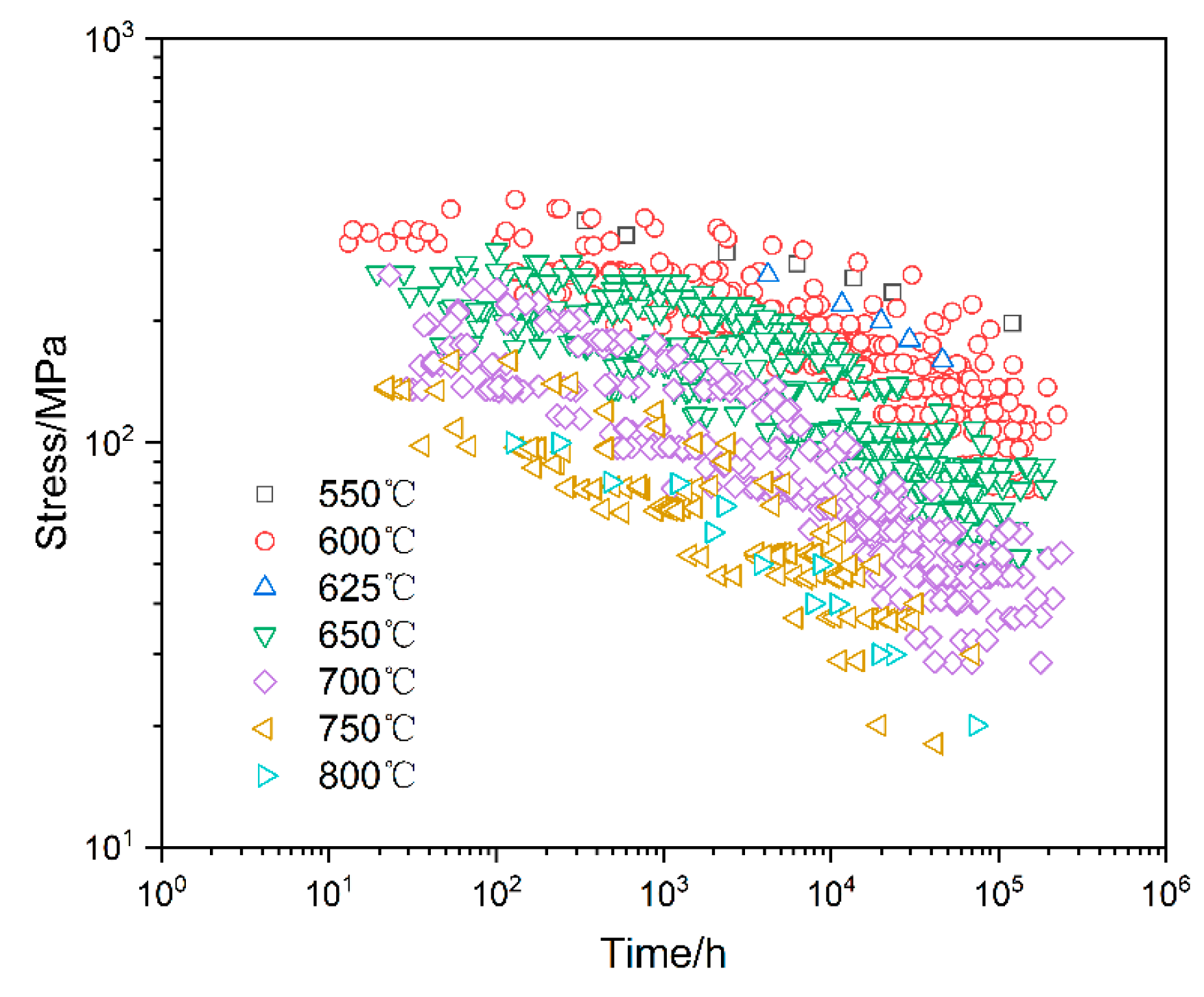
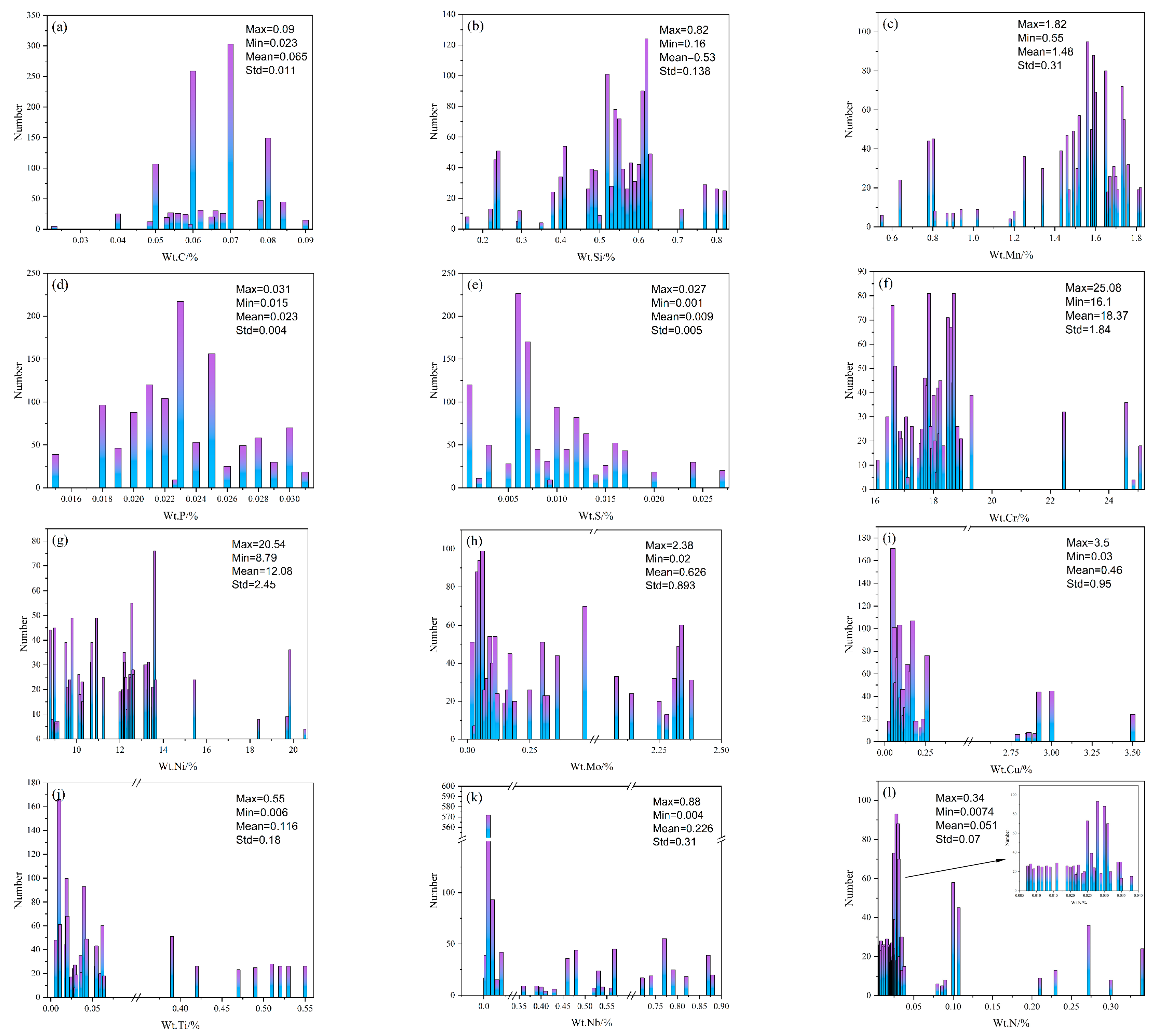
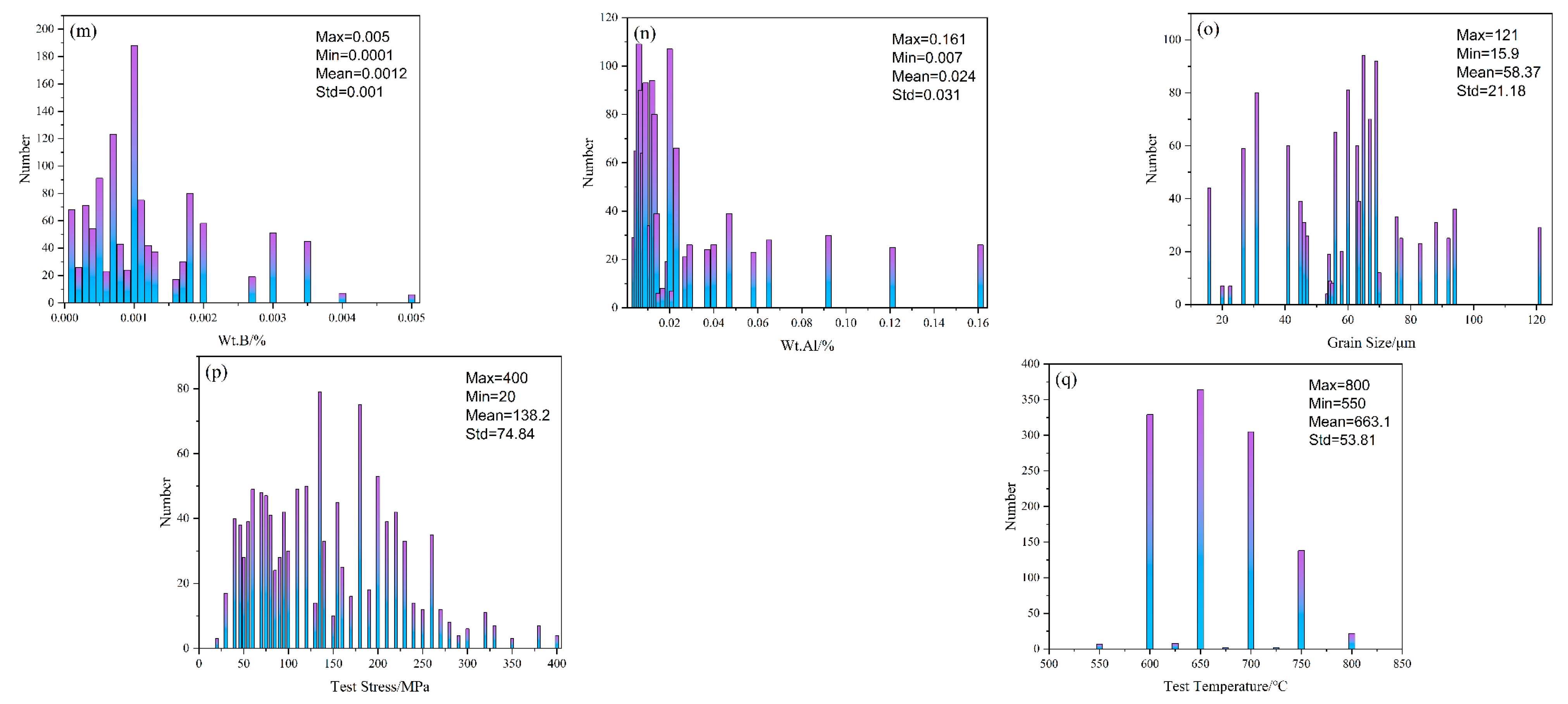
Figure 1 shows the distribution behaviors of the creep life collected for this study. As illustrated in Figure 1, the creep rupture life data are distributed between 10 and 2 × 10⁵ h, the stress data range from 18 to 400 MPa, and the experimental temperature varies between 550 and 800 °C. Moreover, the creep data are obtained from experiments of tube specimens. The following six materials are included in the data: TP304H, TP321H, TP316H, TP347H, S30432, and TP310HCbN [34,35,36,37,38]. A total of 1060 datasets are collected, and the data numbers for each material are 207, 231, 245, 194, 117, and 66, respectively. The characteristic parameters in the data are the chemical composition, the grain size, the test temperature, and the test stress. The data distribution of the characteristic parameters is shown in Figure 2. The x-axis denotes the content of each element within the dataset, while the y-axis represents the frequency of occurrence of an element’s content within the dataset. In general, characteristics such as the compositional features, the processing characteristics, the microstructure, and the experimental conditions are typical input features for life prediction. The materials used in this study are austenitic steels, therefore, the grain size is used as the input feature for the microstructure. The precipitation, as a generated phase during the creep, is one of the important factors affecting the creep properties of austenitic steels. However, the input features of the precipitated phases are unavailable in this study since no data on them are present in the literature to which the dataset belongs. Fortunately, the precipitation and growth of the phase is related to the chemical composition; therefore, the effect of precipitation on creep fracture can be reflected to some extent by the chemical composition as an input feature.
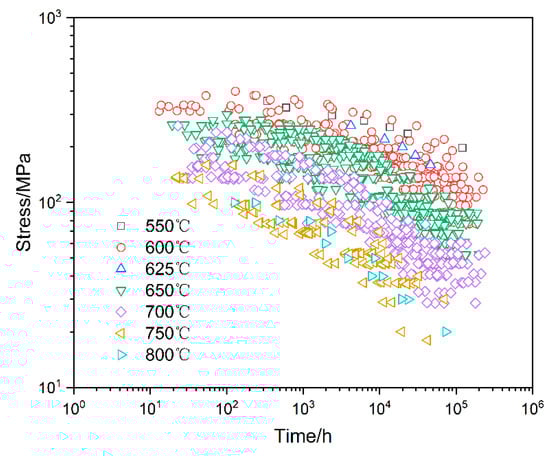
Figure 1.
Creep lifetime distribution in the dataset.

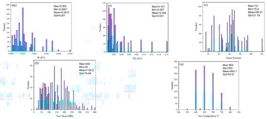
Figure 2.
Distribution of input features in the dataset. ‘max’, ‘min’, ‘mean’, and ‘std’ represent the maximum, minimum, average, and standard deviation, respectively. (a) C; (b) Si; (c) Mn; (d) P; (e) S; (f) Cr; (g) Ni; (h) Mo; (i) Cu; (j) Ti; (k) Nb; (l) N; (m) B; (n) Al; (o) grain size; (p) test stress; and (q) test temperature.
2.2. Feature Extraction and Dataset Creation
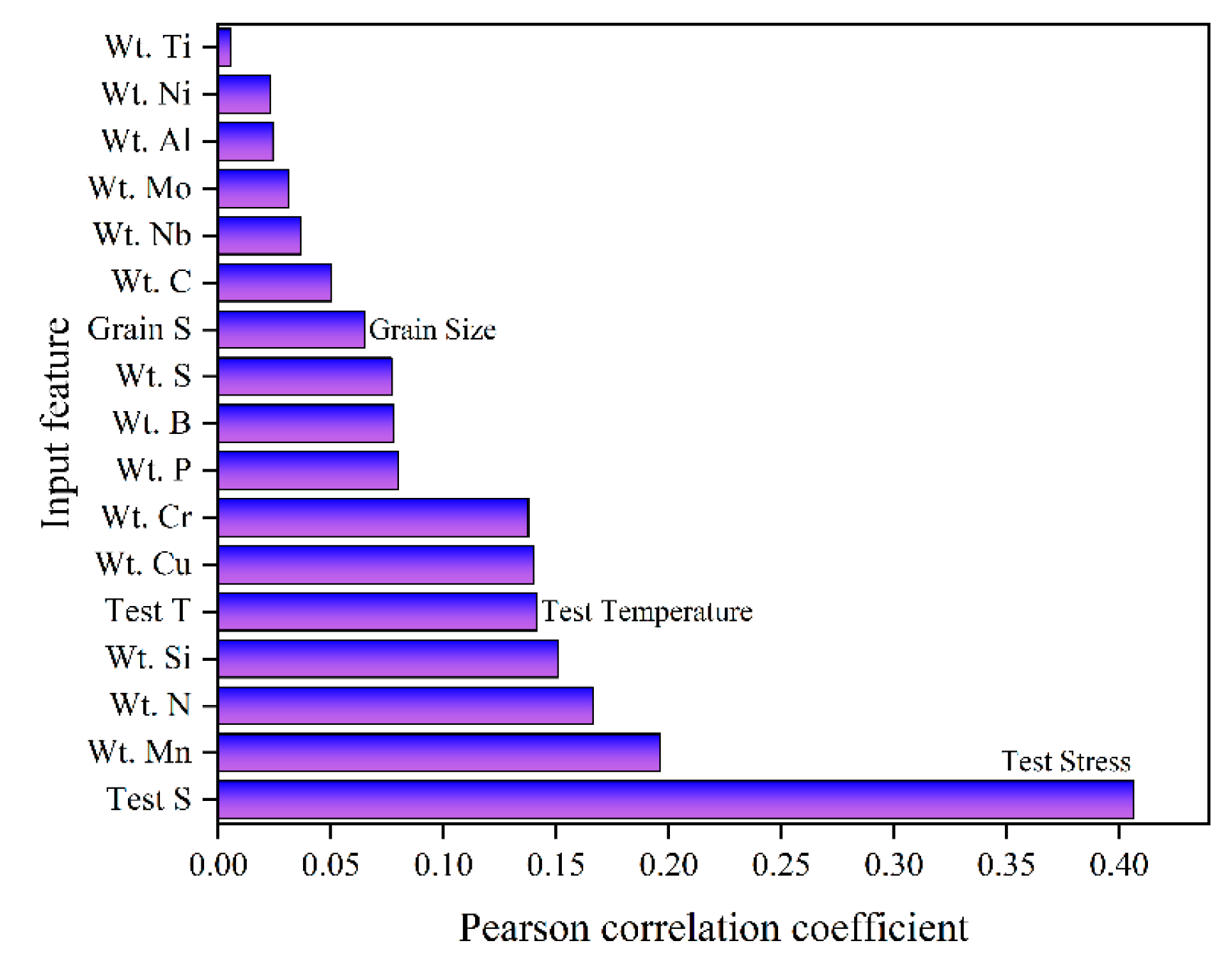
Sensitivity analysis is a statistical technique used to investigate the degree and direction of the linkages between two or more characteristic variables. In this study, Pearson’s correlation coefficient is used to investigate the effect of various input characteristic coefficients on the creep rupture time of austenitic steel. The formula is as follows:
where Cov stands for covariance; Var represents variance; Xi represents the austenitic-steel-influencing factor attribute, where I ranges from 1 to 17; and Y denotes the creep fracture time attribute. The Pearson’s correlation coefficient ranges from −1 to 1; furthermore, a correlation coefficient closer to 1 indicates a stronger impact of the variable on creep fracture life.
Figure 3 presents the correlation coefficients between the various input features and the creep rupture time for the austenitic steels. It shows that all of the feature coefficients have correlation coefficients of <0.5, indicating that the creep rupture time of the austenitic steels is affected by the non-linear interaction of several feature coefficients. In other words, establishing an accurate relationship between the creep life and the features is not possible when the input features are small. Furthermore, the correlation coefficient for the test stress (Test S) is the highest among all of the input features, and it is twice as high as the second highest coefficient. There are essentially equivalent correlation coefficients for the contents of the elements Mn, N, Si, Cu, and Cr, and the test temperature (Test T). The correlation coefficients for the input features, other than those mentioned above, exhibit a small value.
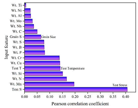
Figure 3.
Correlation coefficient between input features and creep life.
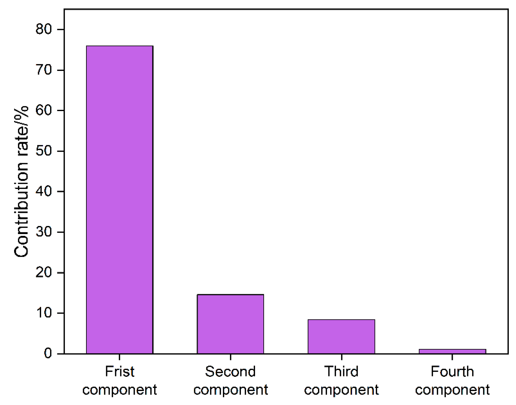
As shown in Figure 2, a total of 17 types of input parameters related to the creep fracture are identified in this study. Generally, the input feature’s high dimensionality may result in a disaster of dimensionality or overfitting on the machine learning model. Reducing the input features from a high-dimensional space to a low-dimensional space is essential and can be achieved through the Principal Component Analysis (PCA) method. By obtaining low-latitude input features in this manner, the main information of the input attributes is retained, and noise reduction is achieved. Figure 4 illustrates that 17 types of input features are transformed into 4 classes of principal components after the PCA processing. The first principal component can express over 75% of the information from the original set of features. Furthermore, by combining the first and second principal components, over 90% of the data can be expressed. Three datasets are constructed based on the results of the Principal Component Analysis (PCA), as presented in Table 1. We treat the first principal component as a separate dataset, the second dataset consists of the first and second principal components, and the third dataset encompasses all of the features.

Figure 4.
Contributions of different principal components.

Table 1.
Grouping and composition of dataset.
2.3. Data Preprocessing
The input features of the dataset show that the values of the different data classes are significantly variable. In order to reduce their impact on model training and improve the training speed, the normalization of the input features is required. In this study, the values of the different input features are transformed into the interval [0, 1] by normalization.
2.4. Selection and Evaluation of the Machine Learning Model
Machine learning algorithms, as a whole, are divided into unsupervised and supervised learning. For lifetime prediction, a regression algorithm with supervised learning is most appropriate. This section evaluates the performance of five candidate machine learning algorithms in order to determine the best prediction model for the creep fracture life of austenitic steel. The five methods are the Support Vector Machine (SVM), integrated learning (Ensemble), Gaussian Regression (Gaussian), Decision Tree (DT), and the BP Neural Network (BPNN). Generally, the ability of a model to predict generalization to unknown data is a measure of its applicability. The training dataset is 80% of the total dataset, i.e., 848 datapoints, and the rest are the test dataset. Moreover, the training dataset is not partitioned into the training and validation datasets. A 10-fold cross-validation method is used to assess the generalization ability of the model during the training of the dataset. To assess the model performance using cross-validation, the initial dataset is subjected to 200 divisions, modeling, and predictions, in order to eliminate the random errors generated by a single training and test set division for model prediction. The prediction error of the algorithm is then determined as the minimum of the 200 model errors observed. Finally, the test dataset is employed to assess the generalization capability of the models. In addition, the predictive performance of the model was assessed using the coefficient of determination (R2), as demonstrated in Equation (2).
where and represent the experimental creep life and the creep life predicted by the model for austenitic steels, respectively. Additionally, represents the average of all of the experimental values.
3. Results and Discussion
3.1. Predictive Results of the Machine Learning Methods
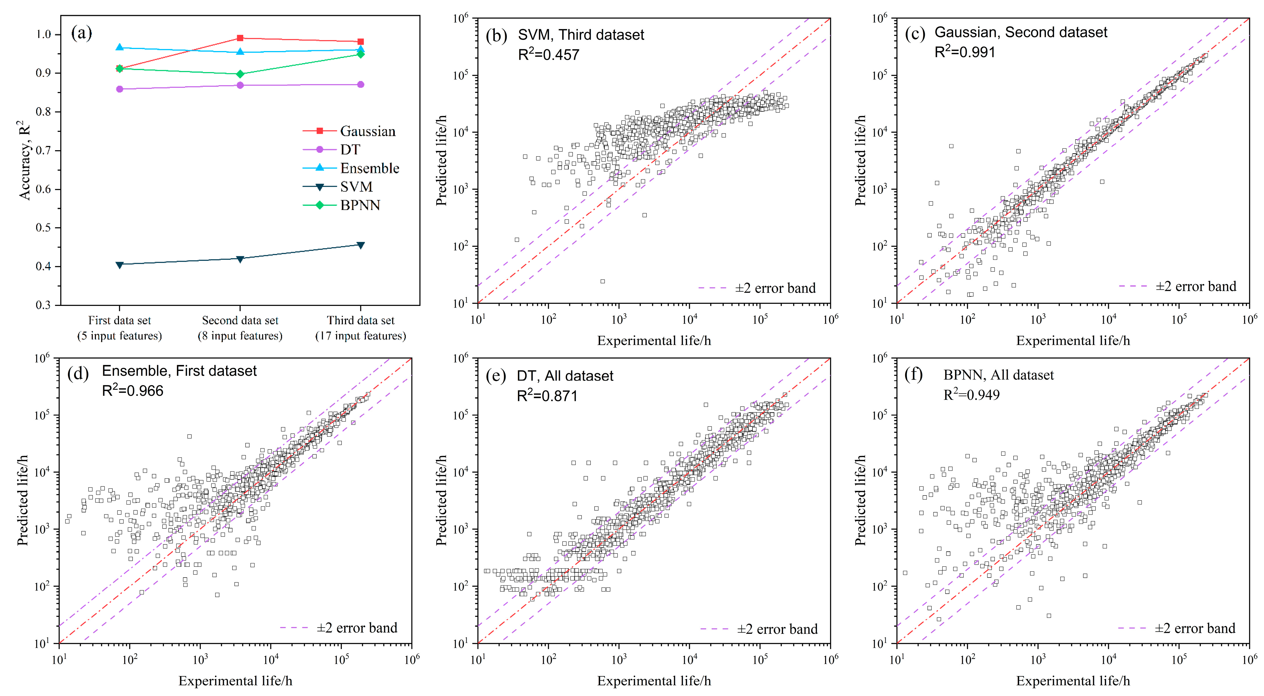
Figure 5a shows a comparison of the prediction accuracy of the machine learning models after being trained on various datasets. It is evident from Figure 5a that the SVM model provides a low prediction accuracy of 0.40–0.48. Moreover, as the number of input features in the dataset increases, the prediction accuracy of the SVM model gradually improves. Nonetheless, the other four prediction models exhibit superior prediction accuracy in comparison to the SVM model. Similar to the SVM model, the prediction accuracy of the Gaussian, Ensemble, and BPNN models varies with the size of the dataset. When the number of input features in the dataset increases, the accuracy of the Gaussian model predictions first increases and then decreases. At the second dataset, it achieves its highest prediction accuracy of 0.998. Both the Ensemble model and the BPNN model show a pattern of decreasing and increasing. The Ensemble model displays the highest accuracy at the first dataset, while the BPNN model achieves the highest accuracy at the third dataset. In contrast to the above models, the prediction accuracy of the DT model remains relatively stable with increasing input features and is between 0.85 and 0.86. In general, based on the predictive accuracy scores, the models are ranked as follows: Gaussian (second dataset) > Ensemble (first dataset) > BPNN (third dataset) > DT (third dataset) > SVM (third dataset). Moreover, this indicates that enhancing the dimensions of the input features in the database does not necessarily enhance the accuracy of the prediction. Enhancing the accuracy of the prediction necessitates matching the input feature dimensions with the prediction model.
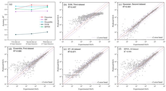
Figure 5.
Predicted life of machine learning models with different datasets. (a) Prediction accuracy of machine learning models; (b) SVM, Third dataset; (c) Gaussian, Second dataset; (d) Ensemble, First dataset; (e) DT, Third dataset; and (f) BPNN, Third dataset.
Figure 5b,f illustrates a comparison between the predicted and the experimental values for the different models’ highest prediction accuracies. Using 104 h as a threshold, the data longer than or equal to 104 h are considered part of the long-life interval, while data shorter than that are considered part of the short-life interval. As shown in Figure 5b, a notable discrepancy exists between the anticipated and the actual SVM model outcomes over the full-life interval. Additionally, a mere 40% of the total data fall within the ±2 error boundaries. In the long-life data, the predicted values of the Gaussian model are in agreement with the experimental values, except for a few individual datapoints that lie outside of the ±2 error band (Figure 5c). The difference between the predicted and the experimental values increases, especially for the short lifetime intervals, particularly those of ≤103 h. The Ensemble and BPNN models demonstrate minor variations in the predicted values when compared to the experimental data for the long-life interval. Over 90% of the data predicted by both of the models fall within the ±2 error limit; however, their accuracy is still weaker than that of the Gaussian model (Figure 5d,e). Furthermore, just like the Gaussian model, both of the models exhibit noticeable variation from the experimental results when it comes to predicting the short-life data. Unlike the above models, the prediction accuracy of the DT model over the full-life interval does not differ much, as shown in Figure 5f. Over the full-life interval, more than 80% of the predicted data fall within the ±2 error band. However, the predictions of the DT model are more discrete within the ±2 error band than the predictions made by the Gaussian, Ensemble, and BPNN models for the long-life interval.
3.2. Comparison of Predictive Results Using Machine Learning and the Conventional Method
There are two commonly used methods for predicting the creep fracture life of austenitic steels: the isotherm method and the LM parametric method. The isotherm method predicts the creep rupture life at a given temperature based only on the persistence time of the different stresses. In contrast, the LM parametric method considers the effects of stress, time, and temperature variations. The LM method connects the three previously mentioned variables using the following equation:
where T is the experimental temperature, t is the creep rupture time, C is the LM constant to be determined, and k is the exponent of the higher order term of the polynomial, k = 2 [9,27]. In addition, b0, b1, and b2 are the parameters to be fitted.
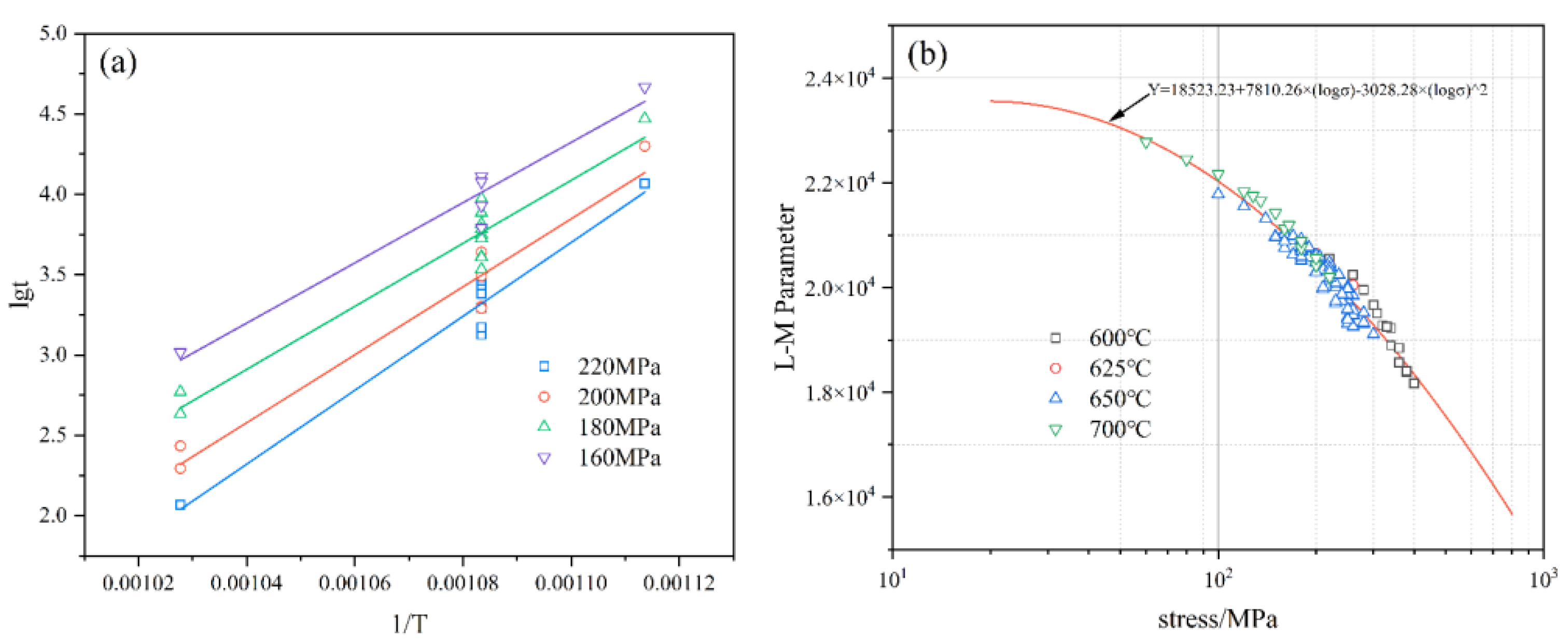
A comparison of the prediction results of machine learning and the conventional methods using S30432 steel is used as an example here. Figure 6a presents the lgt vs. 1/T plot for the LM constant C using the intersection method. Additionally, the data used in the plot include information from the literature [38] and from our research group. The figure shows C-values for 220, 200, 180, and 160 MPa as 16.29585, 17.47969, 19.41373, and 21.6, respectively. To obtain the average C-value, Cave, we take the arithmetic mean of the above values as Cave = 18.6973. Furthermore, the parameters of the LM are fitted with b0 = 18523.23, b1 = 7810.26, and b2 = −3028.28, according to Equation (3), which is illustrated in Figure 6b.
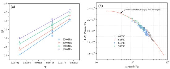
Figure 6.
Acquisition of the LM model parameters. (a) Plot of lgt vs. 1/T and (b) fit curve of the LM model.
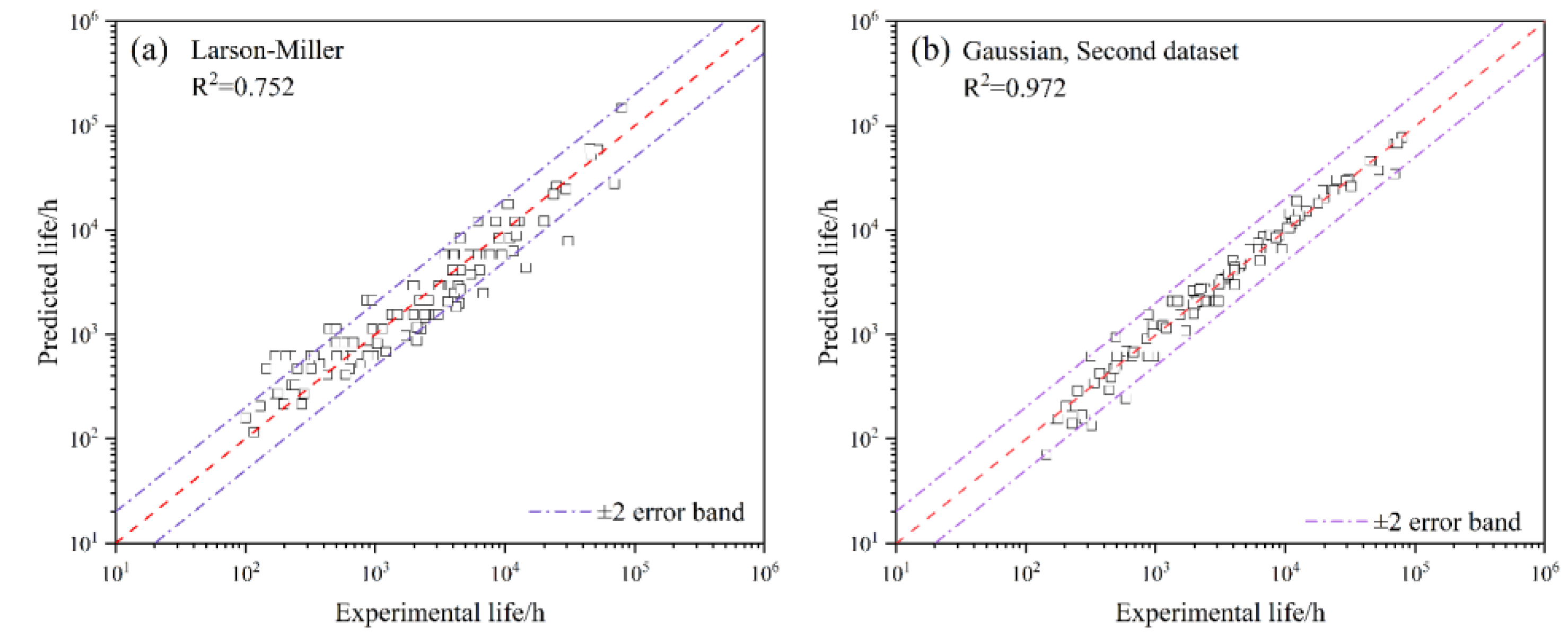
Figure 7 shows the predicted creep life of S30432 austenitic steel using various methods. It illustrates that the conventional LM method predicts high dispersion, with an accuracy of 0.752, while the Gaussian model, based on the second dataset, predicts a high accuracy of 0.972. Additionally, the LM method is based on a dataset of S30432 steel, while the Gaussian model utilizes a dataset that includes various austenitic steels. Compared to the LM model, the machine learning Gaussian model exhibits superior prediction accuracy and steel grade adaptability.
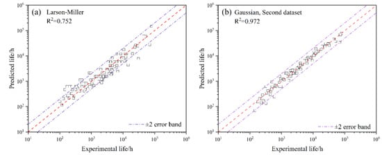
Figure 7.
The predicted life of LM model and Gaussian model. (a) LM model and (b) Gaussian model.
3.3. Effect of Input Features on Creep Fracture Lifetime
To improve the creep life of austenitic steel, introducing alloy atoms into the matrix, optimizing the morphology of austenite, and regulating the precipitation of the second phase can be effective strategies. In this section, the influences of the element content and the grain size on the creep life of S30432 austenitic steel are investigated. Equation (4) is used to normalize the different characteristic parameters to the interval [0, 1], since their variation range is not consistent. The normalization is used to convert the different characteristic parameters to the interval [0, 1].
where x represents the relative amount of input features after normalization, Mx is the actual amount of an input feature, and Mmax and Mmin are the maximum and minimum values of an input feature, respectively, taken from the ASME SA-213M standard [39].
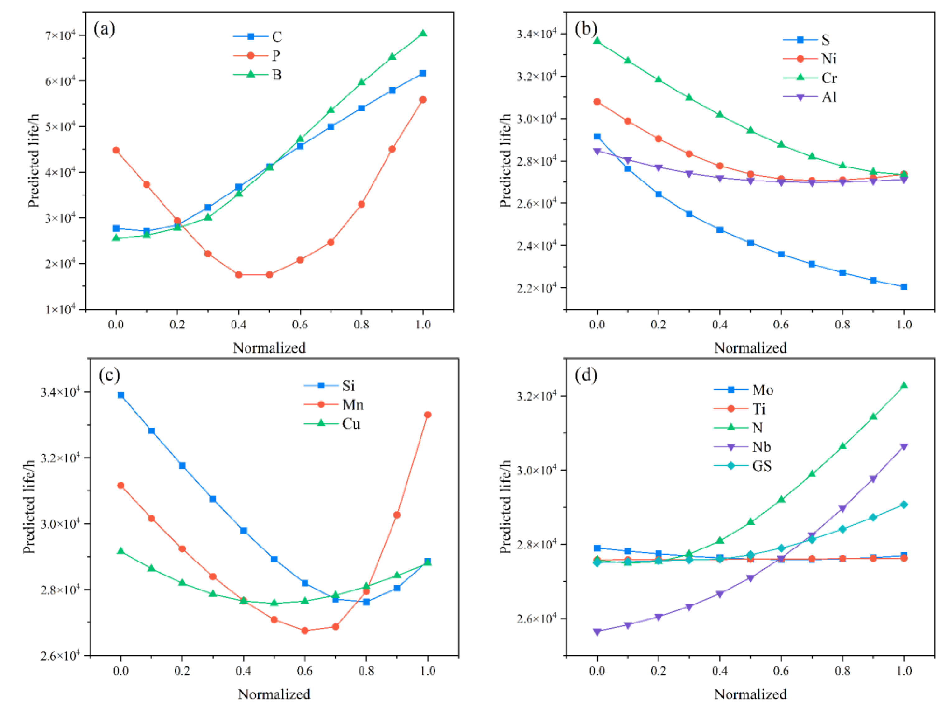
The trend in the impact of various input characteristics on the creep rupture life is shown in Figure 8. In general, the lifespan of S30432 steel varies significantly between 15,000 h and 70,000 h, as the contents of C, P, and B elements vary. Comparatively, the impact of the changes in the other characteristics on the lifespan of S30432 steel is relatively limited.
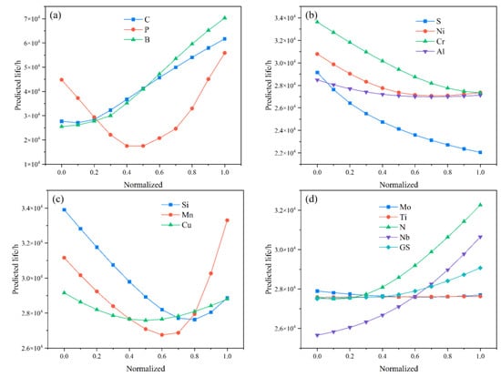
Figure 8.
Effect of different input characteristics on creep life. (a) C, P, and B; (b) S, Ni, Cr, and Al; (c) Si, Mn, and Cu; and (d) Mo, Ti, N, Nb, and GS (grain size).
According to Figure 8b, the creep life of S30432 steel decreases with the continuous increase in concentrations of Cr, Ni, Al, and S. As a general rule, when the level of Cr content rises, it inhibits the MX and M2CN precipitates; however, as for Ni, it inhibits the MX, the σ phase, and the Cu-rich phase [40,41]. Al has a strong affinity for both O and N and has the capability to refine the S30432 grains. However, an increase in Al reduces the bonding of N with the other alloying elements, such as Cr and Nb. Therefore, all three of the elements mentioned above reduce the precipitation strengthening effect of the precipitates in the steel. An increase in the S content may result in the formation of FeS and MnS at the grain boundaries, leading to weakened grain boundary bonding. Consequently, the high-temperature creep properties of the material may reduce.
Figure 8a,c indicates that the creep life initially decreases and then increases as the content of P, Cu, Mn, and Si increases. The research has revealed that the addition of a specific amount (0.1–0.3 mass%) of P promotes the precipitation of M23C6 and, consequently, increases the creep strength of the steel [35,42]. Meanwhile, Cu is distributed diffusely in the form of the Cu-rich phase in the matrix during the high-temperature creep, thereby enhancing the creep strength of the steel [41]. However, the effect of Cu is predicted to decrease and then increase, which is at variance with reality. This may be caused by the overly concentrated distribution of Cu data in the dataset. In contrast to P and Cu, the function mechanism of Mn and Si primarily affects the stacking fault energy of the steel. This indicates that Si reduces the stacking fault energy of the steel, whereas Mn increases it [43]. From the view of improving the creep strength, the Si content should be increased, while reducing the Mn content. However, an increase in Si increases the chance of ferrite nucleation, while a reduction in Mn has a detrimental effect on the austenite stabilization [44,45]. Thus, the two elements must be adequately proportioned in order to improve the creep strength.
It can be observed in Figure 8a,d that the creep life of the S30432 steel is positively correlated with the elemental contents of C, B, N, and Nb. Moreover, the Ti and Mo element contents have a minimal impact on the creep life of the S30432 steel. C, N, B, and Nb all contribute to the formation of the main precipitation strengthening phases (M23C6, MX) of the S30432 steel. An increase in their concentration promotes the nucleation of the precipitated phases. The Mo element has a significant impact on the corrosion properties of the S30432 steel, while Ti plays a crucial role in the deoxidation and fixing of carbon and nitrogen elements during steelmaking; however, both Mo and Ti elements have a minor effect on the creep properties of the S30432 steel. In general, the effect of the second phase on the creep life presented in the above analyses is a general phenomenon and excludes exceptional cases, including significant growth and merging of precipitation, the emergence of the second phases through atypical heat treatments, an unusual second phases added externally, etc.
According to Figure 8d, with increasing austenite grain size, the creep life gradually increases. The dataset reveals that the creep experiments were conducted at temperatures exceeding the isotropic temperature (approximately ≥ 0.5 Tm, Tm: melting point of the steel) of the austenitic steels [46]. At this time, the grain boundary strength is lower than that of the intragranular strength, and the creep mechanism is dominated by grain boundary slip. Consequently, increasing the grain size may reduce the grain boundary occupancy ratio and decrease the chance of cracks occurring due to grain boundary slip. This improves the creep life of the material.
4. Conclusions
In present work, five machine learning models are used to predict the creep life of austenitic stainless steels. The prediction results from the Gaussian model are compared with those from the conventional LM methods. Furthermore, the effect of different input features on the creep life of steel is investigated, using S30432 steel as an example. The main conclusions obtained are as follows:
- The prediction accuracy of the machine learning models varies widely. Moreover, the prediction accuracy varies with different datasets. The Gaussian (second dataset) model has the highest prediction accuracy (0.991), while the SVM (third dataset) model has the lowest prediction accuracy (0.457).
- The Gaussian (second dataset) model has a high prediction accuracy (0.972) and is suitable for the life prediction of a wide range of austenitic steels, as compared to the conventional LM methods.
- The machine-learning -predicted patterns of input features on the creep life are in general agreement with the results of experimental observations and theoretical analyses. In order to improve the creep life, it is advisable to increase the grain size (GS) and the amounts of C, B, and Nb, while decreasing the amounts of Cr, Ni, Al, and S. It is also important to monitor and limit the amounts of P, Cu, Mn, and Si to ensure that they do not fall within the mid-range of the ASME standard [39].
Author Contributions
L.W.: Resources, Methodology, Writing—original draft, Writing—review and editing, Validation, and Formal analysis. S.W.: Software and Validation. W.H.: Data curation. J.H.: Data curation. N.Q.: Resources, Methodology, and Validation. Y.L.: Supervision and Validation. J.Z.: Conceptualization, Supervision, and Project administration. All authors have read and agreed to the published version of the manuscript.
Funding
This work is supported by the National Key Research and Development Program of China, grant number 2021YFC3001803, and the Natural Science Foundation of Heilongjiang Province of China, grant number LH2022E076.
Data Availability Statement
The data and codes that support the findings of this study are available from the corresponding author upon reasonable request.
Conflicts of Interest
The authors declare that they have no known competing financial interests or personal relationships that could have appeared to influence the work reported in this paper.
References
- Spindler, M.W.; Andersson, H. ECCC Rupture Data for Austenitic Stainless Steels—Experiences Gained with Demanding Data Analyses. In Proceedings of the 5th International Conference on Advances in Materials Technology for Fossil Power Plants, Marco Island, FL, USA, 3–5 October 2007. [Google Scholar]
- Igarashi, M.; Semba, H.; Yonemura, M.; Hamaguchi, T.; Okada, H.; Yoshizawa, M.; Iseda, A. Advances in Materials Technology for USC Power Plant Boilers. In Proceedings of the Advances in Materials Technology for Fossil Power Plants-Proceedings from the 6th International Conference, Santa Fe, NM, USA, 31 August–3 September 2011. [Google Scholar]
- Ghatak, A.; Robi, P.S. Modification of Larson–Miller Parameter Technique for Predicting Creep Life of Materials. Trans. Indian Inst. Met. 2015, 69, 579–583. [Google Scholar] [CrossRef]
- Gustin, A.Z.; Zuzek, B.; Podgornik, B. Creep Life Prediction of 10CrMo9-10 Steel by Larson-Miller Model. Materials 2022, 15, 4431. [Google Scholar] [CrossRef] [PubMed]
- Cheng, L.; Guo, Q.; Yu, W.; Han, Y.; Cai, Q. Comparative Study of θ Projection Method and Its Modified Forms on Creep Life Prediction. Steel Res. Int. 2023, 94, 2200270. [Google Scholar] [CrossRef]
- Fu, C.; Chen, Y.; Yuan, X.; Tin, S.; Antonov, S.; Yagi, K.; Feng, Q. A modified θ projection model for constant load creep curves-I. Introduction of the model. J. Mater. Sci. Technol. 2019, 35, 223–230. [Google Scholar] [CrossRef]
- Fu, C.; Chen, Y.; Yuan, X.; Tin, S.; Antonov, S.; Yagi, K.; Feng, Q. A modified θ projection model for constant load creep curves-II. Application of creep life prediction. J. Mater. Sci. Technol. 2019, 35, 687–694. [Google Scholar] [CrossRef]
- Evans, M. A new statistical framework for the determination of safe creep life using the theta projection technique. J. Mater. Sci. 2011, 47, 2770–2781. [Google Scholar] [CrossRef]
- Salifu, S.; Desai, D.; Kok, S. Numerical simulation and creep-life prediction of X20 steam piping. Mater. Today Proc. 2021, 38, 893–898. [Google Scholar] [CrossRef]
- Li, Z.; Wen, Z.; Pei, H.; Yue, X.; Wang, P.; Ai, C.; Yue, Z. Creep life prediction for a nickel-based single crystal turbine blade. Mech. Adv. Mater. Struct. 2021, 29, 6039–6052. [Google Scholar] [CrossRef]
- Goyal, S.; Laha, K. Creep life prediction of 9Cr–1Mo steel under multiaxial state of stress. Mater. Sci. Eng. A 2014, 615, 348–360. [Google Scholar] [CrossRef]
- He, J.; Sandström, R. Modelling grain boundary sliding during creep of austenitic stainless steels. J. Mater. Sci. 2015, 51, 2926–2934. [Google Scholar] [CrossRef]
- Wen, J.-F.; Tu, S.-T. A multiaxial creep-damage model for creep crack growth considering cavity growth and microcrack interaction. Eng. Fract. Mech. 2014, 123, 197–210. [Google Scholar] [CrossRef]
- Viswanathan, G.; Vasudevan, V.; Mills, M. modification of the jogged screw model for creep of TiAl. Acta Mater. 1999, 47, 1399–1411. [Google Scholar] [CrossRef]
- Nabarro, F.R.N. Creep in commercially pure metals. Acta Mater. 2006, 54, 263–295. [Google Scholar] [CrossRef]
- He, J.; Sandström, R. Creep cavity growth models for austenitic stainless steels. Mater. Sci. Eng. A 2016, 674, 328–334. [Google Scholar] [CrossRef]
- Durodola, J.F. Machine learning for design, phase transformation and mechanical properties of alloys. Prog. Mater. Sci. 2022, 123, 100797. [Google Scholar] [CrossRef]
- Li, M.; Mesbah, M.; Fallahpour, A.; Nasiri-Tabrizi, B.; Liu, B. Mechanical strength estimation of ultrafine-grained magnesium implant by neural-based predictive machine learning. Mater. Lett. 2021, 305, 130627. [Google Scholar] [CrossRef]
- Mesbah, M.; Fattahi, A.; Bushroa, A.R.; Faraji, G.; Wong, K.Y.; Basirun, W.J.; Fallahpour, A.; Nasiri-Tabrizi, B. Experimental and Modelling Study of Ultra-Fine Grained ZK60 Magnesium Alloy with Simultaneously Improved Strength and Ductility Processed by Parallel Tubular Channel Angular Pressing. Met. Mater. Int. 2019, 27, 277–297. [Google Scholar] [CrossRef]
- Xie, Q.; Suvarna, M.; Li, J.; Zhu, X.; Cai, J.; Wang, X. Online prediction of mechanical properties of hot rolled steel plate using machine learning. Mater. Des. 2021, 197, 109201. [Google Scholar] [CrossRef]
- Wang, L.; Liu, X.; Fan, P.; Zhu, L.; Zhang, K.; Wang, K.; Song, C.; Ren, S. A creep life prediction model of P91 steel coupled with back-propagation artificial neural network (BP-ANN) and θ projection method. Int. J. Press. Vessel. Pip. 2023, 206, 105039. [Google Scholar] [CrossRef]
- Tan, Y.; Wang, X.; Kang, Z.; Ye, F.; Chen, Y.; Zhou, D.; Zhang, X.; Gong, J. Creep lifetime prediction of 9% Cr martensitic heat-resistant steel based on ensemble learning method. J. Mater. Res. Technol. 2022, 21, 4745–4760. [Google Scholar] [CrossRef]
- Wang, J.; Fa, Y.; Tian, Y.; Yu, X. A machine-learning approach to predict creep properties of Cr–Mo steel with time-temperature parameters. J. Mater. Res. Technol. 2021, 13, 635–650. [Google Scholar] [CrossRef]
- Han, H.; Li, W.; Antonov, S.; Li, L. Mapping the creep life of nickel-based SX superalloys in a large compositional space by a two-model linkage machine learning method. Comput. Mater. Sci. 2022, 205, 111229. [Google Scholar] [CrossRef]
- Chai, M.; He, Y.; Li, Y.; Song, Y.; Zhang, Z.; Duan, Q. Machine Learning-Based Framework for Predicting Creep Rupture Life of Modified 9Cr-1Mo Steel. Appl. Sci. 2023, 13, 4972. [Google Scholar] [CrossRef]
- Zhang, X.C.; Gong, J.G.; Xuan, F.Z. A physics-informed neural network for creep-fatigue life prediction of components at elevated temperatures. Eng. Fract. Mech. 2021, 258, 108130. [Google Scholar] [CrossRef]
- Zhang, X.C.; Gong, J.G.; Xuan, F.Z. A deep learning based life prediction method for components under creep, fatigue and creep-fatigue conditions. Int. J. Fatigue 2021, 148, 106236. [Google Scholar] [CrossRef]
- Gu, H.H.; Wang, R.Z.; Zhu, S.P.; Wang, X.W.; Wang, D.M.; Zhang, G.D.; Fan, Z.C.; Zhang, X.C.; Tu, S.T. Machine learning assisted probabilistic creep-fatigue damage assessment. Int. J. Fatigue 2022, 156, 106677. [Google Scholar] [CrossRef]
- Ferreño, D.; Serrano, M.; Kirk, M.; Sainz-Aja, J.A. Prediction of the Transition-Temperature Shift Using Machine Learning Algorithms and the Plotter Database. Metals 2022, 12, 186. [Google Scholar] [CrossRef]
- Rasmussen, C.E. Gaussian Processes in Machine Learning. In Advanced Lectures on Machine Learning; Bousquet, O., von Luxburg, U., Rätsch, G., Eds.; Lecture Notes in Computer Science; Springer: Berlin/Heidelberg, Germany, 2003; Volume 3176. [Google Scholar] [CrossRef]
- Mitra, S.; Konwar, K.M.; Pal, S.K. Fuzzy decision tree, linguistic rules and fuzzy knowledge-based network: Generation and evaluation. IEEE Trans. Syst. Man Cybern. Part C (Appl. Rev.) 2002, 32, 328–339. [Google Scholar] [CrossRef]
- Kohonen, T. An Introduction to Neural Computing. Neural Netw. 1988, 1, 3–16. [Google Scholar] [CrossRef]
- Burges, C.J. A Tutorial on Support Vector Machines for Pattern Recognition. Data Min. Knowl. Discov. 1998, 2, 121–167. [Google Scholar] [CrossRef]
- Abe, F.; Tanaka, H.; Murata, M. Effect of Nb on long-term creep life of JIS SUS304HTB and JIS SUS347HTB steels –heat-to-heat variation and life assessment of stainless steels. Mater. High Temp. 2016, 33, 626–635. [Google Scholar] [CrossRef]
- Matsuo, T.; Shinoda, T.; Tanaka, R. Effect of Nitrogen, Boron and Phosphorous on High Temperature Strength of 18Cr-10Ni and 18Cr-10NiMo Austenitic Steels Bearing Small Amounts of Titanium and Niobium. Tetsu Hagane 1973, 59, 907–918. [Google Scholar] [CrossRef] [PubMed]
- Abe, F. Heat-to-Heat Variation in Creep Life and Fundamental Creep Rupture Strength of 18Cr-8Ni, 18Cr-12Ni-Mo, 18Cr-10Ni-Ti, and 18Cr-12Ni-Nb Stainless Steels. Metall. Mater. Trans. A 2016, 47, 4437–4454. [Google Scholar] [CrossRef]
- Hatakeyama, T.; Sawada, K.; Sekido, K.; Hara, T.; Kimura, K. Influence of dynamic microstructural changes on the complex creep deformation behavior of 25Cr–20Ni–Nb–N steel at 873 K. Mater. Sci. Eng. A 2021, 814, 141270. [Google Scholar] [CrossRef]
- Kimura, K.; Sawada, K. Creep Deformation Property and Creep Life Evaluation of Super304H. J. Press. Vessel. Technol. 2022, 144, 021507. [Google Scholar] [CrossRef]
- An International Code 2021 ASME Boiler & Pressure Vessel Code. ASME SA-213/ SA-213M Specification for Seamless Ferritic and Austenitic Alloy- Steel Boiler, Superheater, and Heat-Exchanger Tubes; American Society of Mechanical Engineers: New York, NY, USA, 2021; pp. 285–300. [Google Scholar]
- Ou, P.; Xing, H.; Wang, X.; Sun, J.; Cui, Z.; Yang, C. Coarsening and Hardening Behaviors of Cu-Rich Precipitates in Super304H Austenitic Steel. Metall. Mater. Trans. A 2015, 46, 3909–3916. [Google Scholar] [CrossRef]
- Bai, J.W.; Liu, P.P.; Zhu, Y.M.; Li, X.M.; Chi, C.Y.; Yu, H.Y.; Xie, X.S.; Zhan, Q. Coherent precipitation of copper in Super304H austenite steel. Mater. Sci. Eng. A 2013, 584, 57–62. [Google Scholar] [CrossRef]
- Froes, F.H.; Wells, M.G.H.; Banerjee, B.R. Influence of Phosphorus on the Nucleation of M23C6 Carbides in Austenitic Stainless Steels. Met. Sci. J. 1968, 2, 232–234. [Google Scholar] [CrossRef]
- Li, D.; Feng, Y.; Song, S.; Liu, Q.; Bai, Q.; Ren, F.; Shangguan, F. Influences of silicon on the work hardening behavior and hot deformation behavior of Fe–25 wt%Mn–(Si, Al) TWIP steel. J. Alloys Compd. 2015, 618, 768–775. [Google Scholar] [CrossRef]
- Lai, J.K.L.; Shek, C.H.; Lo, K.H. (Eds.) Stainless Steels: An Introduction and Their Recent Developments; Bentham Science Publishers: Sharjah, Sharjah, United Arab Emirates, 2012. [Google Scholar]
- Xiong, R.; Peng, H.; Wang, S.; Si, H.; Wen, Y. Effect of stacking fault energy on work hardening behaviors in Fe–Mn–Si–C high manganese steels by varying silicon and carbon contents. Mater. Des. 2015, 85, 707–714. [Google Scholar] [CrossRef]
- Dai, Y.; Kong, Q. On the Physical Origin of Equicohesive Temperature for Creep. Strength Met. Alloys 1989, 2, 959–964. [Google Scholar] [CrossRef]
Disclaimer/Publisher’s Note: The statements, opinions and data contained in all publications are solely those of the individual author(s) and contributor(s) and not of MDPI and/or the editor(s). MDPI and/or the editor(s) disclaim responsibility for any injury to people or property resulting from any ideas, methods, instructions or products referred to in the content. |
© 2023 by the authors. Licensee MDPI, Basel, Switzerland. This article is an open access article distributed under the terms and conditions of the Creative Commons Attribution (CC BY) license (https://creativecommons.org/licenses/by/4.0/).