Article

On the Use of Machine Learning Algorithms to Predict the Corrosion Behavior of Stainless Steels in Lactic Acid

Mechanical Engineering Department, École de technologie supérieure, 1100, Rue Notre-Dame Ouest, Montréal, QC H3C 1K3, Canada
*
Author to whom correspondence should be addressed.
Metals 2023, 13(8), 1459; https://doi.org/10.3390/met13081459
Submission received: 7 July 2023 / Revised: 9 August 2023 / Accepted: 11 August 2023 / Published: 13 August 2023
(This article belongs to the Special Issue Corrosion Prediction in Different Environment)

Abstract

:
Predicting the corrosion behavior of materials in specific environmental conditions is important for establishing a sustainable manufacturing system while reducing the need for time-consuming experimental investigations. Recent studies started to explore the application of supervised Machine Learning (ML) techniques to forecast corrosion behavior in various conditions. However, there is currently a research gap in utilizing classification ML techniques specifically for predicting the corrosion behavior of stainless steel (SS) material in lactic acid-based environments, which are extensively used in the pharmaceutical and food industry. This study presents a ML-based prediction model for corrosion behavior of SSs in different lactic acid environmental conditions, using a database that described the corrosion behavior by qualitative labels. Decision tree (DT), random forest (RF) and support vector machine (SVM) algorithms were applied for classification. Training and testing accuracies of, respectively 97.5% and 92.5% were achieved using the DT classifier. Four SS alloy composition elements (C, Cr, Ni, Mo), acid concentration, and temperature were found sufficient to consider as input data for corrosion prediction. The developed models are reliable for predicting corrosion degradation and, as such, contribute to avoiding failures and catastrophes in industry.

1. Introduction

A material’s chemical composition and various environmental or operational factors, including temperature, pH, chloride content [1,2], humidity [3,4], stray currents [5], oxygen levels [6], and impurity levels [7] have a significant impact on corrosion processes. Therefore, it is difficult to link individual environmental factors to corrosion processes or predict corrosion lifetimes from physics-based corrosion laws. Predicting corrosion behavior of materials in any given environmental condition is important, because testing materials in each possible environmental condition is time-consuming and expensive [8]. In addition, analyzing corrosion data and predicting corrosion behavior needs advanced data mining methods [9,10]. The predictive capability of corrosion behavior in stainless steel (SS), which is widely employed in various industries, plays a crucial role in maintaining sustainable manufacturing processes and mitigating the detrimental effects of corrosion [11,12]. The present study focuses on the corrosion behavior prediction of different SSs in a lactic acid environment. This type of corrosive environment is typical for applications in health-related industries such as food, pharmaceuticals, and cosmetics [12,13,14].
In the field of materials research, machine learning (ML) techniques have gained significant popularity due to their effective data mining abilities [9]. Instead of relying on pre-established equations, ML algorithms learn from input data and previous experiences. ML techniques like Random Forest (RF), Support Vector Regression (SVR), and Artificial Neural Networks (ANN) have recently found application in corrosion research to explore corrosion behavior [8,10,15,16]. ML algorithms can be divided into two categories: unsupervised learning and supervised learning. Typically, in unsupervised learning the data has no labels, thus the model must generate a reasonable output without external support. In supervised learning processes, a network is provided with the desired output. Here, the output for specific inputs should be available to train the model and find the mapping function, and then the model can be used to predict the output of new inputs [17].
To model corrosion processes, supervised ML algorithms are mainly deployed. In such cases, typically, the chemical composition of the alloy and environmental factors are considered as input features, and the corrosion rate is considered as output to establish a ML-based corrosion rate prediction model [9,10,15]. Supervised ML techniques are applied in corrosion research for various objectives. These include predicting corrosion rates [16,18,19,20], forecasting pitting corrosion behavior [8], and modeling the maximum dimensions of pits [21]. Additionally, ML methods are utilized to explore the corrosion behavior by considering the underlying physic-based corrosion laws in physic-based models. These models utilize various physical factors associated with corrosion, such as material properties, temperature, salinity, humidity, and more, in order to establish a deterministic relationship [22]. As an example, Shi et al. [23], have used Arrhenius equation in the ANN, which relates the rate of chemical reactions (corrosion) to temperature and activation energy, providing insight into how temperature affects stress corrosion crack growth rates of Inconel alloy 600.
Literature reports various applications of ML in corrosion research, including data visualization, simulation, correlation analysis, and multivariate fitting. ML techniques offer distinct advantages over traditional regression analysis methods [24,25]. ML algorithms can handle diverse features, perform robust regression analyses, and effectively generalize data sets of any scale [26]. Consequently, ML enables in-depth investigations into corrosion behavior and enhances the prediction capabilities through improved technical conditions.
Typically, supervised ML techniques were used to predict corrosion behavior, and the technique was selected based on the size and the type of dataset. Most of the studies applied regression methods and ANNs for prediction [18,23,27,28]. However, there is a lack of research using classification ML techniques, and analyzing their performance for predicting corrosion behavior. Although, often, in practical use cases, datasets are classified based on labels, which needs classification-based predictive models to assign a class label to input numerical data.
Hence, the main objective of this contribution is to determine and evaluate whether categorized (i.e., labeled) datasets are applicable and accurate for prediction of corrosion behavior using classification methods. The studied algorithms include Decision Tree (DT), RF, and Support Vector Machine (SVM), as a classification problem can typically be solved using one of these supervised ML algorithms [29]. As presented in Figure 1a, a DT algorithm has the structure of a tree and is used for classification and prediction. It contains root and internal nodes (non-leaf nodes), which are used to separate instances based on their features. Internal nodes are the result of attributed test cases and leaf nodes (or terminal nodes) denoting the class label [30]. The SVM algorithm applies supervised learning techniques, utilizing support vectors to identify an optimal hyperplane that separates classes within the n-dimensional plane, enabling accurate predictions [31]. In Figure 1b, a two-dimensional data set is considered as a sample, and the hyperplane divides the training data represented by red circles and blue squares. As shown in Figure 1c, in the RF algorithm, multiple randomized DTs are combined, and their predictions are aggregated as a final class [32]. RF is capable of handling high-dimensional data and non-linear classification tasks [33]. Indeed, DTs are widely employed for classification tasks due to their simplicity, interpretability, and capacity to handle both numerical and categorical features. Given the mixed feature types in the dataset of this study, DTs offer a straightforward approach to capture and comprehend the decision-making process, enabling the extraction of meaningful insights from the model [34]. In addition, RF is utilized as an ensemble learning method to address overfitting and check the possible enhancement in the overall accuracy. Generally, by combining multiple decision trees and aggregating their predictions, RF demonstrates a tendency to generalize well on unseen data, making it a suitable choice for improving the model’s robustness and performance [35]. Furthermore, SVM is a powerful classifier renowned for its effectiveness in high-dimensional spaces and ability to handle complex decision boundaries [31]. Considering the presence of multiple features and potentially ©ntricate relationships between them in the dataset of this study, SVM was selected to explore non-linear decision boundaries and establish a competitive baseline for comparison with other algorithms.
This study proposes the use of classification methods to categorize and predict the SS alloys’ corrosion behavior based on the literature data published in the ASM Handbook of Corrosion Data (2nd edition) [38]. The dataset’s features comprise the chemical composition of SS alloys, which includes 13 elements, the electrolyte temperature and the concentration of lactic acid in the electrolytic solution. Various corrosion behaviors within this dataset were qualitatively labeled as Resistant, Good, Poor, and Questionable, with each label defined as follows:
  • Resistant: Corresponding to a mass loss rate of less than 0.1 g/h/m2 or less than 0.11 mm/year decrease in thickness.
  • Good: Corresponding to a mass loss rate ranges from 0.1 to 1.0 g/h/m2 or 0.11 to 1.10 mm/year decrease in thickness.
  • Poor: Corresponding to a mass loss rate ranges from 1.0 to 10.0 g/h/m2 or 1.1 to 11.0 mm/year decrease in thickness.
  • Questionable: Corresponding to a mass loss rate exceeding 10.0 g/h/m2 or 11.0 mm/year decrease in thickness, or being susceptible to local corrosion, pitting, crevice, or stress corrosion.
On this dataset, it was proposed to develop and apply ML classification techniques that map the chemical composition of steel, acid concentration, and temperature to a label, which was defined based on the corrosion rate. Different ML techniques were analyzed by comparing their accuracies. The effect of feature selection and reduction on the accuracy of the models was studied. Finally, the prediction accuracy was improved using hyperparameter tuning techniques.

2. Methodology

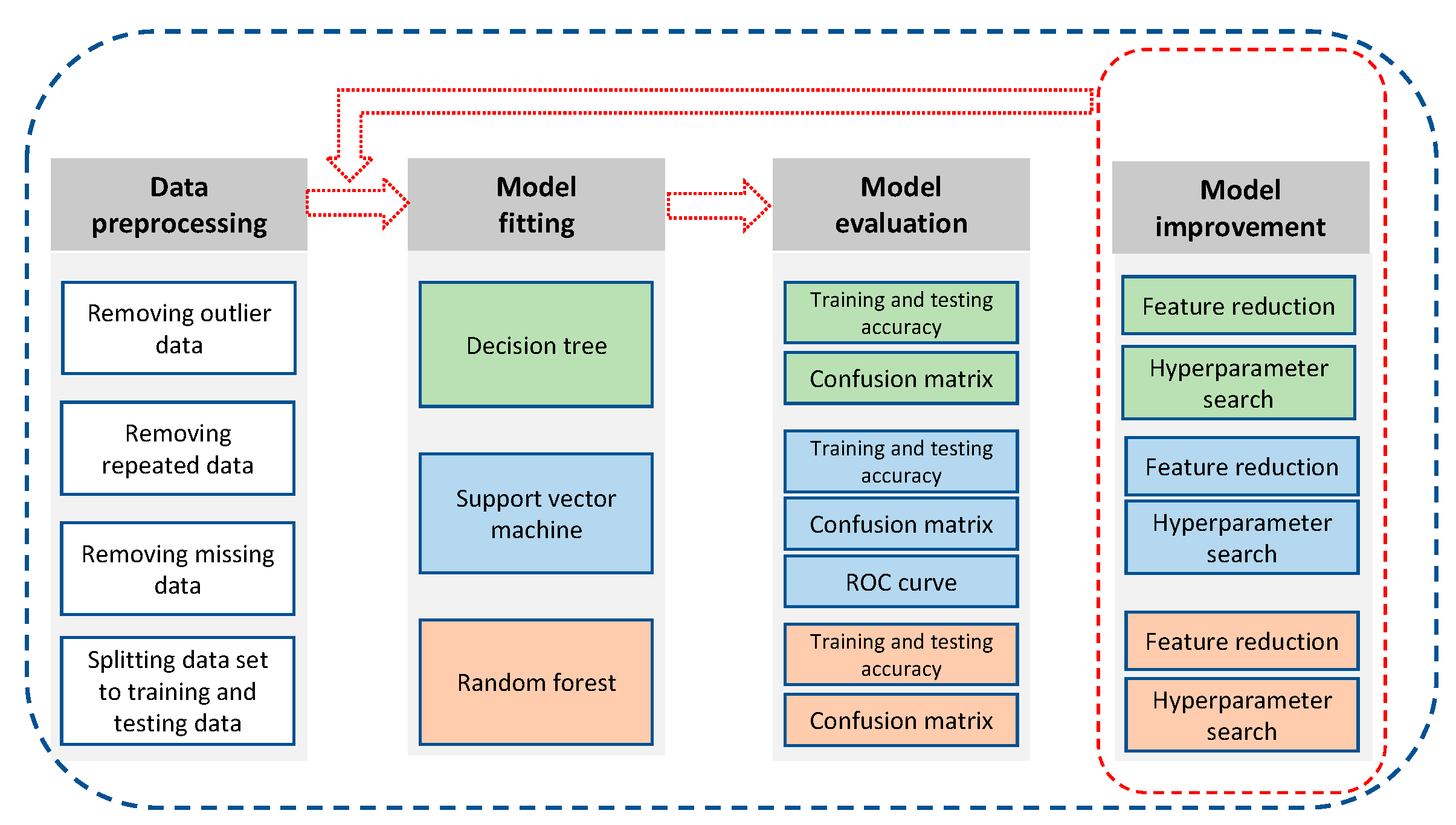
Figure 2 illustrates a schematic representation of the proposed methodology for assessing the corrosion condition of SSs in lactic acid. In the first step, the corrosion data are preprocessed before being transferred to the modeling step. Three ML algorithms, including DT, RF, and SVM, are considered as classification methods. After fitting the model, its performance is assessed by computing training and testing accuracies. Additionally, the models are evaluated using the confusion matrix and Receiver Operator Characteristic (ROC) curves to provide a comprehensive assessment. Hyperparameter tuning is conducted to optimize the model’s hyperparameters, leading to subsequent enhancements in the model’s performance [17]. In addition, feature selection is performed based on the importance of input features to improve the model performance by maintaining high accuracies, while using fewer inputs.
The following Section 2.1, Section 2.2 and Section 2.3 provide the details of the database, the preprocessing methods, the fitted models, and the feature reduction methods utilized in the developed classification ML.

2.1. Corrosion Data Preprocessing

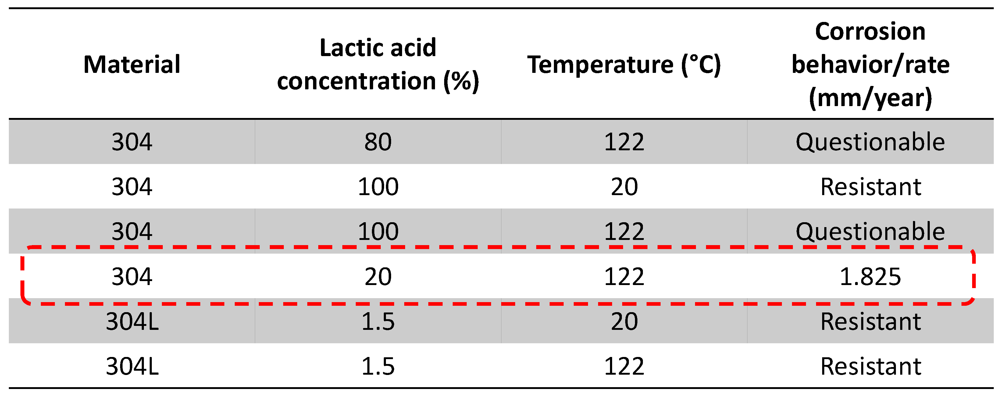
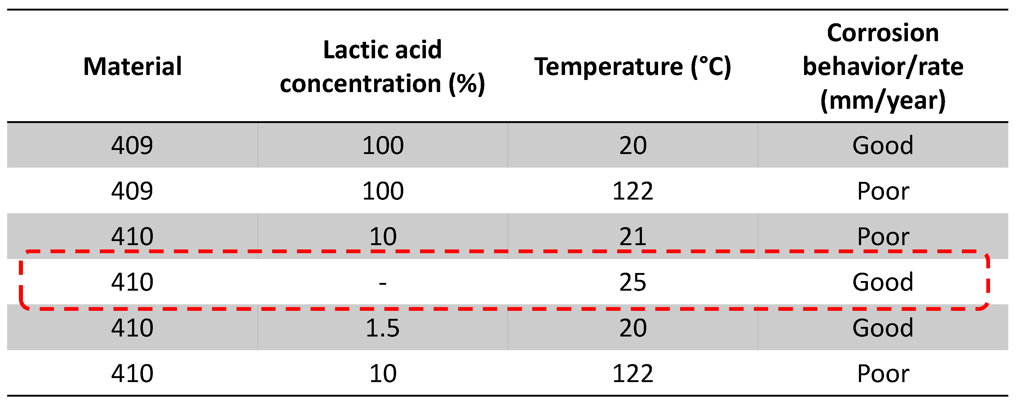
It is necessary to prepare the dataset for ML approaches with the help of preprocessing techniques. At first, the database underwent a uniformity check. The majority of the corrosion behavior labels are qualitative; however, as the experimental data provided in the handbook originated from different references, some data were not qualitative (see the red box in Figure 3) and the corrosion rate was reported numerically in these cases. For a few data series, some features were missing, shown as a red box in Figure 4, where the lactic acid concentration was not reported and, consequently, they were removed from the database. Hence, these undesirable data were removed in the first step of preprocessing to make a uniform dataset. After these manipulations, 198 rows of data were obtained in total.
The chemical compositions of SSs were obtained from the literature [39]. This resulted in the definition of 15 features: 13 representing the elemental compositions in the SS alloy (Table 1), and two features indicating the environmental conditions (electrolyte temperature and acid concentration) as shown in Table 2. The corrosion behavior is also listed in Table 2 as the output feature.

2.2. ML Approach

This study compares the performance of corrosion rate prediction of different ML algorithms, including DT, SVM, and RF. For these three training methods, respectively 80% and 20% of the data are considered as training and testing data sets. As shown in Table 3, four classes of corrosion behavior present in this database and the number of available data for each class is: Resistant—95 labels, Good—58 labels, Poor—22 labels, and Questionable—23 labels. The symbolic labels, Questionable, Poor, Good, and Resistant, are quantified automatically by defining a function label_encoder. The performance of each model was assessed by calculating its test and train accuracy using the sklearn.metrics.accuracy_score function from the Scikitlearn library [40]. For each model, a confusion matrix was generated to examine misclassified labels. The training set was created using two variables, x_train and y_train, and a DT classifier was trained on these variables with random_state = 0. Also, the maximum DT depth was set to the default value max_depth = None to expand nodes until all leaves are pure (i.e., there is only one class on that node). Based on the plotted DT, with max_depth = 10, the lowest class impurity was achieved. Hyperparameter tuning led to a tuned set of parameters with max_depth = 5 and criterion = ‘gini’. In the next step, K-fold cross validation [40] was applied, where the data were divided into k = (2, 3, …, 11) equally sized chunks and each chunk had its turn “pretending” to be a test set. Comparing these validation results with the obtained test accuracies, it can be concluded that the K-fold cross validation is a reasonable and conservative estimate of the testing accuracies for the used ML approaches.
Initially, the SVM model was fitted on the training data using the default hyperparameters (C = 1 and gamma = ‘scale’) with a kernel of ‘rbf’. Subsequently, hyperparameter tuning was conducted to enhance the model’s accuracy. This tuning involved inspecting the regularization parameter C and the kernel coefficient gamma with a reciprocal random distribution. The resulting optimized hyperparameters were found to be C = 1.38 and gamma = 0.019. After applying the SVM algorithm, the RF algorithm was also employed for comparison. To do so, the RF Classifier with random_state = 0 was fitted to the training data. A hyperparameter tuning process was performed to determine the best number of trees in the forest (n_estimators) for this algorithm. The optimal number of estimators, in this case, was identified as 8 for RF classification. It is important to note that further increasing the parameter n_estimators did not yield any positive influence on the accuracy of the model.
The ROC curve is a common and effective method to visualize the performance of the classifier [41,42]. To draw the ROC curve, the false positive rate (FPR) and true positive rate (TPR) values, as shown in Equations (1) and (2) below, were evaluated.
T P R = T p T p + F n
F P R = F p F p + T n
Here, Tp represents the correctly classified known positives (“True positives”), Tn represents the correctly classified known negatives (“True negatives”), Fp represent the incorrectly classified known positives (“False positives”), and Fn represents the incorrectly classified known negatives (“False negatives”). In order to draw a ROC curve for a multiclassification problem, binarization is applied to the data series. Therefore, the function label_binarize from the sklearn.preprocessing library [40] was deployed.

2.3. Feature Reduction

Model development and training for predictive modelling problems can be slow due to the large number of involved variables. To reduce the number of input variables, related features can be selected according to their effectiveness for predicting the target variable (here: corrosion behavior). Some models perform worse when the target variable has a low correlation with the input variables [43]. Therefore, the main reason for feature selection and reduction is to increase the classification accuracy and decrease the training time. As we have numerical input and classified output, the most common feature selection technique is the analysis of variance (ANOVA) [44,45,46]. In this study, the most related features for training models were adopted using the ANOVA feature selection method.

3. Results and Discussion

In this section, the training and testing accuracies for each model are reported separately. To visualize the erroneous predictions, the confusion matrixes and the ROC curves are constructed. In addition, the influence of feature reduction on the accuracy of the models is presented.

3.1. DT Model

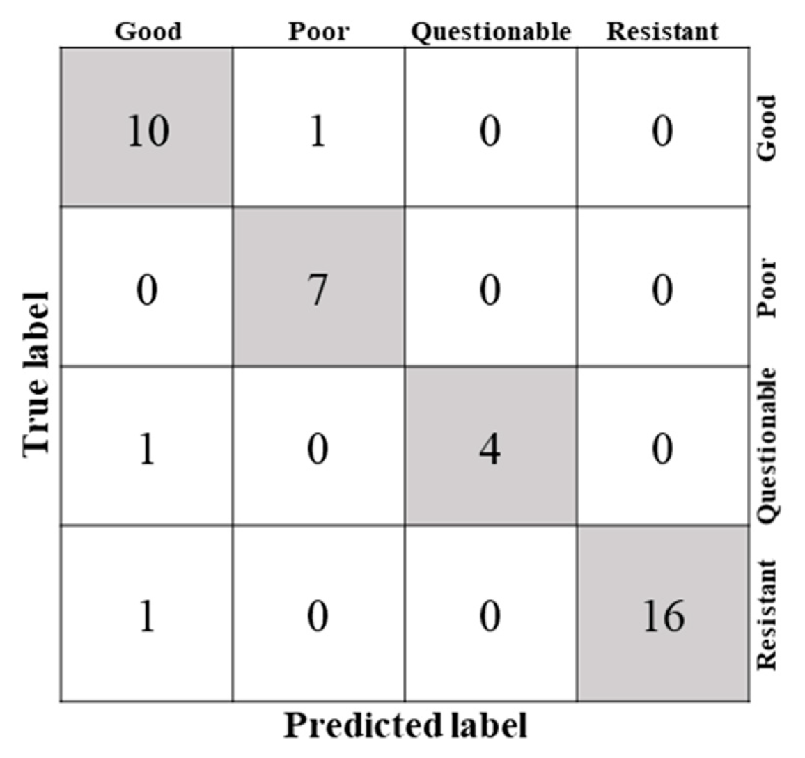
The training and testing accuracies of the developed DT model, calculated by sklearn.metrics.accuracy_score [40], are 98.73% and 90.00%, respectively. After the hyperparameter tuning and using the optimized parameters, the obtained accuracies changed to 97.47% and 92.50%. The confusion matrix (Figure 5) visualizes the number of correct and wrong predictions for each category. In each row, the sum of horizontal values represents the total data series associated with its corrosion label. In other words, in the testing data set, there are 11 datapoints with a Good label, 7 datapoints with a Poor label, 5 datapoints with a Questionable label, and 17 datapoints with a Resistant label. For the data series corresponding to the Good label, 10 of them are classified correctly (Tp), and one is mislabeled by Poor (Fn). For the data series with Questionable and Resistant labels, one Fn classification with a Good label was made. All data series with Poor labels are Tp and are therefore classified correctly.
The DT classifier achieved an average accuracy of 83.92% across all 11 folds with a standard deviation of 5.5%. These results demonstrate the stability and consistency of the model’s performance during cross-validation. It is worth noting that the model exhibits consistent performance across different folds, indicating a good level of generalization. No overfitting is observed, as the performance on the validation sets remained relatively close to the training set accuracy.

3.2. RF Model

The training and testing accuracies of the applied RF model are, respectively, 98.10% and 87.50%. In Figure 6, the confusion matrix shows that all Poor and Questionable labels, which corresponds to an undesired corrosion behavior, were correctly classified. However, some mislabeling for Good and Resistant labels did occur. In other words, the Fn for the Good and Resistant labels are equal to 2 and 3, respectively.

3.3. SVM Model

Considering the default hyperparameter values for the SVM model, the obtained training and testing accuracies are, respectively, 60.13% and 55.00%, which indicates a low performance of this model on the dataset. Figure 7a indicates that none of the Good and Poor classes were classified correctly by the model, and all of them were mistakenly predicted (Fn) as Questionable and Resistant. After applying the hyperparameter tuning, the accuracies improved to 93.04% and 87.50%, respectively. Figure 7b also shows an improvement in detecting the right label for each class. All the Resistant classes are predicted correctly in the dataset; however, some errors in predicting the right label for Good, Questionable, and Poor classes still remain.
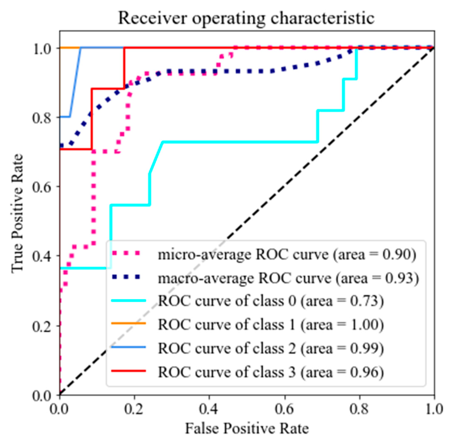
Figure 8 presents a ROC curve for the developed SVM multi-class model, where each curve represents a class (here: class 0 to class 3). The area under each ROC curve represents the degree of separability; the closer this area is to 1, the higher is the capability of distinguishing between classes. For the specific class of TPR equaling 1, all data belonging to that class were classified correctly. In the case of a class with FPR equaling 0, not a single data was considered erroneous for this class. The ROC curve of Figure 8, representing the corrosion behavior of SS in lactic acid, demonstrates that all the Poor labels were correctly classified, and the area under the Questionable curve is very close to 1. Indeed, this is of great importance for practical use, because wrongly classified Poor or Questionable classes (i.e., when wrongly classified as Good or Resistant) may result in a disaster such as failure of systems, accidents and leakage of hazardous substances in industrial applications exposed to corrosive environments.

3.4. Feature Reduction

Due to the large number of variables involved in predictive modelling problems, model development and training can be slow. However, input variables can be reduced by selecting features that are most useful for target variable prediction. Moreover, in the database considered for this study, it is not possible to measure the atomic percentage of all elements, so it is preferred to have a simplified model based on a smaller number of elements. Therefore, feature selection and reduction are aimed to increase classification accuracy, decrease training time, and save time and costs for preparing experimental data that are used to train the models. Table 4 shows the list of input features ranked by deploying the ANOVA technique.
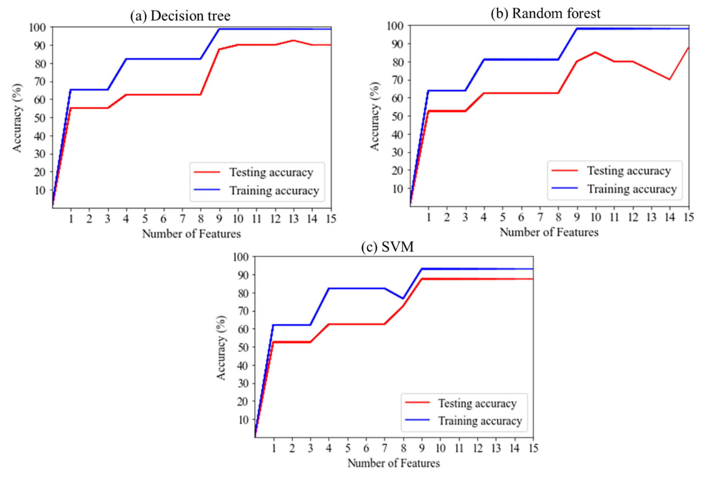
A comparison of training and testing accuracies based on different input numbers for each model (DT, RF and SVM) is shown in Figure 9 to determine the required number of features to be considered as input.
Figure 9 presents the obtained graphs of accuracy versus number of features for each model (Figure 9 (a) DT, (b) RF and (c) SVM). It can be concluded that the highest training accuracy was achieved when considering the first nine features, and further increasing the number of input features has no influence on training accuracy. Testing accuracy varies, specifically for RF, but it can still be considered as stable. Thus, we can conclude from Figure 9 that considering nine input features, including Fe, Ni, Cr, temperature, Mn, C, N, Mo, and lactic acid concentration will provide the same training accuracy compared to considering all 15 input features. The testing accuracy only reduced 2.5%, 7.5%, and 0% for DT, RF and SVM models, respectively. Therefore, feature reduction has a minor impact on the training and testing accuracies. The ROC curves of the SVM models after feature reduction are shown in Figure 10. The latter gives a good indication on how the ML performance is affected. It can be observed that the values remain almost unchanged, indicating no significant influence on the model’s performance.
According to materials science literature, in SS alloys; Ni, Cr, Mo, and C are essential elements in the chemical composition to form corrosion-resistant passive layers [47]. The aforementioned elements are considered to be the most important influencing factors. Thus, feature reduction is also justified from a materials science perspective. It should be highlighted that the feature reduction step, which excludes Si, Al, S, P, Nb, Ta, and Ti elemental composition as input features does not impact prediction accuracy, however, it is not necessarily implying that these elements have no influence on the corrosion behavior of SS in lactic acid. It is important to note that the developed prediction in this study is qualitative, where each label describes a range of corrosion rates, as explained in the introduction Section 1. To comprehensively discuss the effect of the elements Si, Al, S, P, Nb, Ta, and Ti on the corrosion behavior of SSs in lactic acid, conducting experiments and numerical evaluations are necessary next steps in future studies.
ROC curves and accuracy measurements show no major negative impacts after feature reduction. It was proven that the number of inputs can be reduced to keep modeling and prediction faster, and to prepare the experimental data in a more time- and cost-effective manner.

4. Conclusions

In the present study, different ML algorithms were used to model and predict the corrosion behavior of SS alloys in an aqueous environment containing different lactic acid concentrations at varying temperatures. It was demonstrated that using the DT classifier, training and testing accuracies of, respectively, 97.47% and 92.50% could be achieved. The training and testing accuracies of the RF algorithm were 98.1% and 87.5%, respectively, which are close to the DT classifier results. Using the SVM algorithm, a training accuracy of 60.1% and testing accuracy of 55.0% were obtained. To improve the model, hyperparameter tuning was applied, leading to values to 93.0% and 87.5%, respectively. To evaluate the FPR and TPR parameters, an ROC curve for multiclassification was constructed. Based on its graph, it was shown that the area under the curve of the Poor class is equal to 1, which is highly important from a material selection perspective. Finally, ANOVA feature selection was applied to the pre-processed data set and nine input features including Fe, Ni, Cr, temperature, Mn, C, N, Mo, and lactic acid concentration were found as the most influencing factors on the corrosion behavior of SSs in a lactic acid environment. Finally, it can be concluded that SVM, RF, and DT techniques are useful to predict the corrosion behavior of data sets, which consists of quantitative input and qualitative output (labeled) data. The models can predict the corrosion behavior of SS in ‘unseen’ situations (lactic acid concentration and temperature), and then label or classify the corrosion behavior of the material as Poor, Good, Questionable, or Resistant.
Although corrosion engineers prefer to work with quantitative corrosion data, such as corrosion rate or corrosion current density, in some cases, categorization of materials based on their corrosion behavior in different environments is useful and, often, the only information available in practical use cases. This study successfully demonstrates that labeled corrosion behavior of relatively small datasets can be correctly predicted using ML algorithms. In addition, it was observed that, according to the obtained accuracies, DT is the best model to train and test; whereas, according to the confusion matrixes, RF performs best in terms of identifying all Poor and Questionable labels.

Author Contributions

S.P.: Conceptualization, Methodology, Software, Formal analysis, Writing—Original Draft; S.H.: Conceptualization, Methodology, Investigation, Software, Writing—Original Draft; A.-H.B.: Resources, Writing—Review and Editing; L.A.H.: Project administration, Methodology, Resources, Supervision, Writing—Review and Editing. All authors have read and agreed to the published version of the manuscript.

Funding

This research and the APC were funded by the Natural Sciences and Engineering Research Council of Canada (NSERC) through the Discovery Grant (RGPIN-2019-05973 and RGPIN-2021-03780) and École de technologie supérieure.

Data Availability Statement

The raw data that was used and the codes developed to replicate these results can be accessed for download from the provided Github repository: https://github.com/Soroosh-HKN/ML-lactic-acid-corrosion. Accessed on 7 July 2023.

Conflicts of Interest

The authors declare that they have no known competing financial interests or personal relationships that could have appeared to influence the work reported in this paper.

References

  1. Dastgerdi, A.A.; Brenna, A.; Ormellese, M.; Pedeferri, M.P.; Bolzoni, F. Experimental Design to Study the Influence of Temperature, PH, and Chloride Concentration on the Pitting and Crevice Corrosion of UNS S30403 Stainless Steel. Corros. Sci. 2019, 159, 108160. [Google Scholar] [CrossRef] [Green Version]
  2. Wang, Z.; Zhang, L.; Zhang, Z.; Lu, M. Combined Effect of PH and H2S on the Structure of Passive Film Formed on Type 316L Stainless Steel. Appl. Surf. Sci. 2018, 458, 686–699. [Google Scholar] [CrossRef]
  3. Xu, M.; Zhang, Q.; Yang, X.; Wang, Z.; Liu, J.; Li, Z. The Journal of Supercritical Fluids Impact of Surface Roughness and Humidity on X70 Steel Corrosion in Supercritical CO2 Mixture with SO. J. Supercrit. Fluids 2016, 107, 286–297. [Google Scholar] [CrossRef]
  4. Patel, S.; Rogalsky, A.; Vlasea, M. Towards Understanding Side-Skin Surface Characteristics in Laser Powder Bed Fusion. J. Mater. Res. 2020, 35, 2055–2064. [Google Scholar] [CrossRef]
  5. Xu, W.; Li, Y.; Li, H.; Wang, K.; Zhang, C.; Jiang, Y.; Qiang, S. Corrosion Mechanism and Damage Characteristic of Steel Fiber Concrete under the Effect of Stray Current and Salt Solution. Constr. Build. Mater. 2022, 314, 125618. [Google Scholar] [CrossRef]
  6. Huang, S.; Yang, Y.; Li, Z.; Liu, Y.; Su, D. Corrosion Behavior and Mechanism of P110 Casing Steel in Alkaline-Activated Persulfate-Based Preflush Fluid. Eng. Fail. Anal. 2023, 152, 107482. [Google Scholar] [CrossRef]
  7. Sun, J.; Tang, H.; Wang, C.; Han, Z.; Li, S. Effects of Alloying Elements and Microstructure on Stainless Steel Corrosion: A Review. Steel Res. Int. 2022, 93, 2100450. [Google Scholar] [CrossRef]
  8. Jiménez-Come, M.J.; de la Luz Martín, M.; Matres, V. A Support Vector Machine-Based Ensemble Algorithm for Pitting Corrosion Modeling of EN 1.4404 Stainless Steel in Sodium Chloride Solutions. Mater. Corros. 2019, 70, 19–27. [Google Scholar] [CrossRef] [Green Version]
  9. Yan, L.; Diao, Y.; Lang, Z.; Gao, K. Corrosion Rate Prediction and Influencing Factors Evaluation of Low-Alloy Steels in Marine Atmosphere Using Machine Learning Approach. Sci. Technol. Adv. Mater. 2020, 21, 359–370. [Google Scholar] [CrossRef] [Green Version]
  10. Pei, Z.; Zhang, D.; Zhi, Y.; Yang, T.; Jin, L.; Fu, D.; Cheng, X.; Terryn, H.A.; Mol, J.M.C.; Li, X. Towards Understanding and Prediction of Atmospheric Corrosion of an Fe/Cu Corrosion Sensor via Machine Learning. Corros. Sci. 2020, 170, 108697. [Google Scholar] [CrossRef]
  11. Gedge, G. Structural Uses of Stainless Steel—Buildings and Civil Engineering. J. Constr. Steel Res. 2008, 64, 1194–1198. [Google Scholar] [CrossRef]
  12. Zaffora, A.; Di Franco, F.; Santamaria, M. Corrosion of Stainless Steel in Food and Pharmaceutical Industry. Curr. Opin. Electrochem. 2021, 29, 100760. [Google Scholar] [CrossRef]
  13. Moradi, M.; Guimarães, J.T.; Sahin, S. Current Applications of Exopolysaccharides from Lactic Acid Bacteria in the Development of Food Active Edible Packaging. Curr. Opin. Food Sci. 2021, 40, 33–39. [Google Scholar] [CrossRef]
  14. Alsaheb, R.A.A.; Aladdin, A.; Othman, Z.; Malek, R.A.; Leng, O.M.; Aziz, R.; Enshasy, H.A. El Lactic Acid Applications in Pharmaceutical and Cosmeceutical Industries. J. Chem. Pharm. Res. 2015, 7, 729–735. [Google Scholar]
  15. Diao, Y.; Yan, L.; Gao, K. Improvement of the Machine Learning-Based Corrosion Rate Prediction Model through the Optimization of Input Features. Mater. Des. 2021, 198, 109326. [Google Scholar] [CrossRef]
  16. Lv, Y.J.; Wang, J.W.; Wang, J.; Xiong, C.; Zou, L.; Li, L.; Li, D.W. Steel Corrosion Prediction Based on Support Vector Machines. Chaos Solitons Fractals 2020, 136, 109807. [Google Scholar] [CrossRef]
  17. Wang, A.Y.T.; Murdock, R.J.; Kauwe, S.K.; Oliynyk, A.O.; Gurlo, A.; Brgoch, J.; Persson, K.A.; Persson, K.A.; Sparks, T.D. Machine Learning for Materials Scientists: An Introductory Guide toward Best Practices. Chem. Mater. 2020, 32, 4954–4965. [Google Scholar] [CrossRef]
  18. Kamrunnahar, M.; Urquidi-Macdonald, M. Prediction of Corrosion Behavior Using Neural Network as a Data Mining Tool. Corros. Sci. 2010, 52, 669–677. [Google Scholar] [CrossRef]
  19. Wen, Y.F.; Cai, C.Z.; Liu, X.H.; Pei, J.F.; Zhu, X.J.; Xiao, T.T. Corrosion Rate Prediction of 3C Steel under Different Seawater Environment by Using Support Vector Regression. Corros. Sci. 2009, 51, 349–355. [Google Scholar] [CrossRef]
  20. Hakimian, S.; Pourrahimi, S.; Bouzid, A.H.; Hof, L.A. Application of Machine Learning for the Classification of Corrosion Behavior in Different Environments for Material Selection of Stainless Steels. Comput. Mater. Sci. 2023, 228, 112352. [Google Scholar] [CrossRef]
  21. Cavanaugh, M.K.; Buchheit, R.G.; Birbilis, N. Modeling the Environmental Dependence of Pit Growth Using Neural Network Approaches. Corros. Sci. 2010, 52, 3070–3077. [Google Scholar] [CrossRef]
  22. Li, X.; Jia, R.; Zhang, R.; Yang, S.; Chen, G. A KPCA-BRANN Based Data-Driven Approach to Model Corrosion Degradation of Subsea Oil Pipelines. Reliab. Eng. Syst. Saf. 2022, 219, 108231. [Google Scholar] [CrossRef]
  23. Shi, J.; Wang, J.; Macdonald, D.D. Prediction of Primary Water Stress Corrosion Crack Growth Rates in Alloy 600 Using Artificial Neural Networks. Corros. Sci. 2015, 92, 217–227. [Google Scholar] [CrossRef]
  24. Chico, B.; Díaz, I.; Simancas, J.; Morcillo, M. Annual Atmospheric Corrosion of Carbon Steel Worldwide. An Integration of ISOCORRAG, ICP/UNECE and MICAT Databases. Materials 2017, 10, 601. [Google Scholar] [CrossRef] [Green Version]
  25. Cai, Y.; Zhao, Y.; Ma, X.; Zhou, K.; Wang, H. Application of Hierarchical Linear Modelling to Corrosion Prediction in Different Atmospheric Environments. Corros. Eng. Sci. Technol. 2019, 54, 266–275. [Google Scholar] [CrossRef]
  26. Pruksawan, S.; Lambard, G.; Samitsu, S.; Sodeyama, K.; Naito, M. Prediction and Optimization of Epoxy Adhesive Strength from a Small Dataset through Active Learning. Sci. Technol. Adv. Mater. 2019, 20, 1010. [Google Scholar] [CrossRef] [PubMed] [Green Version]
  27. Shi, Y.; Fu, D.; Zhou, X.; Yang, T.; Zhi, Y.; Pei, Z.; Zhang, D.; Shao, L. Data Mining to Online Galvanic Current of Zinc/Copper Internet Atmospheric Corrosion Monitor. Corros. Sci. 2018, 133, 443–450. [Google Scholar] [CrossRef]
  28. Pintos, S.; Queipo, N.V.; Troconis De Rincón, O.; Rincón, A.; Morcillo, M. Artificial Neural Network Modeling of Atmospheric Corrosion in the MICAT Project. Corros. Sci. 2000, 42, 35–52. [Google Scholar] [CrossRef]
  29. Singh, S.; Singhania, S.; Pandya, V.; Singal, A.; Biwalkar, A. East Meets West: Sentiment Analysis for Election Prediction. Stud. Comput. Intell. 2022, 1027, 9–20. [Google Scholar] [CrossRef]
  30. Han, J.; Kamber, M.; Kaufmann, M. Data Mining: Concepts and Techniques, 2nd ed.; Classification and Prediction; Morgan Kaufmann: San Francisco, CA, USA, 2006. [Google Scholar]
  31. Noble, W.S. What Is a Support Vector Machine? Nat. Biotechnol. 2006, 24, 1565–1567. [Google Scholar] [CrossRef]
  32. Gill, S.; Pathwar, P. Prediction of Diabetes Using Various Feature Selection and Machine Learning Paradigms. Stud. Comput. Intell. 2022, 1027, 133–146. [Google Scholar] [CrossRef]
  33. Jalal, N.; Mehmood, A.; Choi, G.S.; Ashraf, I. A Novel Improved Random Forest for Text Classification Using Feature Ranking and Optimal Number of Trees. J. King Saud. Univ.-Comput. Inf. Sci. 2022, 34, 2733–2742. [Google Scholar] [CrossRef]
  34. Safavian, S.R.; Landgrebe, D. A Survey of Decision Tree Classifier Methodology. IEEE Trans. Syst. Man Cybern. 1991, 21, 660–674. [Google Scholar] [CrossRef] [Green Version]
  35. Belgiu, M.; Drăgu, L. Random Forest in Remote Sensing: A Review of Applications and Future Directions. ISPRS J. Photogramm. Remote Sens. 2016, 114, 24–31. [Google Scholar] [CrossRef]
  36. Armaghani, D.J.; Asteris, P.G.; Askarian, B.; Hasanipanah, M.; Tarinejad, R.; Van Huynh, V. Examining Hybrid and Single SVM Models with Different Kernels to Predict Rock Brittleness. Sustainability 2020, 12, 2229. [Google Scholar] [CrossRef] [Green Version]
  37. Mennitt, D.; Sherrill, K.; Fristrup, K. A Geospatial Model of Ambient Sound Pressure Levels in the Contiguous United States. J. Acoust. Soc. Am. 2014, 135, 2746–2764. [Google Scholar] [CrossRef]
  38. Craig, B.D.; Anderson, D.B. Lactic Acid. In Handbook of Corrosion Data, 2nd ed.; ASM International: Almere, The Netherlands, 1995; pp. 488–492. ISBN 978-0-87170-518-1. [Google Scholar]
  39. Society of Automotive Engineers; American Society for Testing and Materials. Metals & Alloys in the Unified Numbering System; SAE International: Warrendale, PA, USA, 2008; p. 583. [Google Scholar]
  40. Pedregosa, F.; Michel, V.; Grisel, O.; Blondel, M.; Prettenhofer, P.; Weiss, R.; Vanderplas, J.; Cournapeau, D.; Pedregosa, F.; Varoquaux, G.; et al. Scikit-Learn: Machine Learning in Python. J. Mach. Learn. Res. 2011, 12, 2825–2830. [Google Scholar]
  41. Hanley, J.A.; McNeil, B.J. The Meaning and Use of the Area under a Receiver Operating Characteristic (ROC) Curve. Radiology 1982, 143, 29–36. [Google Scholar] [CrossRef] [Green Version]
  42. Cortes, C.; Mohri, M. AUC Optimization vs. Error Rate Minimization. Adv. Neural Inf. Process. Syst. 2003, 16, 313–320. [Google Scholar]
  43. Kuhn, M.; Johnson, K. Applied Predictive Modeling; Springer: New York, NY, USA, 2013; pp. 1–600. [Google Scholar]
  44. Lin, H.; Chen, W. Prediction of Thermophilic Proteins Using Feature Selection Technique. J. Microbiol. Methods 2011, 84, 67–70. [Google Scholar] [CrossRef] [PubMed]
  45. Ding, H.; Guo, S.H.; Deng, E.Z.; Yuan, L.F.; Guo, F.B.; Huang, J.; Rao, N.; Chen, W.; Lin, H. Prediction of Golgi-Resident Protein Types by Using Feature Selection Technique. Chemom. Intell. Lab. Syst. 2013, 124, 9–13. [Google Scholar] [CrossRef]
  46. Ding, H.; Feng, P.M.; Chen, W.; Lin, H. Identification of Bacteriophage Virion Proteins by the ANOVA Feature Selection and Analysis. Mol. Biosyst. 2014, 10, 2229–2235. [Google Scholar] [CrossRef] [PubMed]
  47. Olefjord, I.; Elfstrom, B.O. The Composition of the Surface during Passivation of Stainless Steels. Corrosion 1982, 38, 46–52. [Google Scholar] [CrossRef]
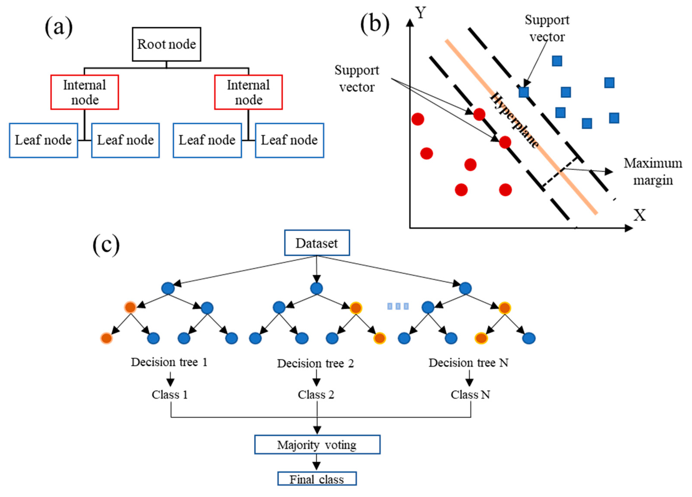
Figure 1. Conceptual diagram of (a) DT algorithm indicating root node, internal nodes, and leaf nodes (inspired from [30]); (b) SVM algorithm in a 2D data set (inspired from [36]); (c) RF algorithm consisting of N decision trees (inspired from [37]).
Metals 13 01459 g001
Figure 2. Diagram illustrating the designed and implemented procedures for classifying and predicting corrosion behavior.
Metals 13 01459 g002
Figure 3. A sample which has a quantified corrosion behavior label is highlighted within the red box (based on database [38]).
Metals 13 01459 g003
Figure 4. A sample which lacks the lactic acid concentration feature is highlighted within the red box (based on database [38]).
Metals 13 01459 g004
Figure 5. Confusion matrix for DT model, presenting the number of Tp and Fn labels.
Metals 13 01459 g005
Figure 6. Confusion matrix for RF, presenting the number of Tp and Fn labels.
Metals 13 01459 g006
Figure 7. Confusion matrix for SVM model (a) before hyperparameter tuning (b) after hyperparameter tuning, presenting the number of Tp and Fn labels.
Metals 13 01459 g007
Figure 8. Receiver operating characteristic (ROC) curve for corrosion behavior labels.
Metals 13 01459 g008
Figure 9. Training and testing accuracies based on number of input features for (a) DT; (b) RF; and (c) SVM.
Metals 13 01459 g009
Figure 10. ROC curve after feature reduction.
Metals 13 01459 g010
Table 1. The chemical composition of the studied SSs [39].
Stainless Steels%C%Mn%Si%P%S%Cr%Mo%Ni%N%Ti%Nb + Ta%Al%Fe
3010.15210.0450.0316-6----74.77
3020.1520.750.050.0317-80.1---71.92
3030.15210.20.3517-8----71.3
3040.0820.750.050.0318-80.1---70.99
304L0.0320.750.050.0318-80.1---71.04
304LN0.0320.750.050.0318-80.16---70.98
3160.0820.750.050.03162100.1---68.99
316L0.0320.750.050.03162100.1---69.04
316LN0.03210.050.03162100.3---68.59
316 Ti0.08210.050.03162100.10.7--68.04
317L0.03210.050.03183110.1---64.79
317LN0.03210.050.03183110.22---64.67
3210.0820.750.050.0317-90.10.7--70.29
3290.05210.050.02251.34.50.05---66.04
3470.08210.050.0317-9--1-69.84
4030.15210.050.0311.5------85.27
4050.08110.050.0311.5-----0.186.24
4090.08110.050.0510.5-0.5-0.7--86.13
4100.15110.050.0311.5-0.75----85.52
4160.151.2510.060.1512------85.39
4200.15110.050.0312------85.77
4300.12110.050.0316------81.8
4340.08110.050.03160.75-----81.09
F510.03210.050.03212.54.50.08---68.81
Table 2. Features list used in models for the corrosion classification.
FeatureUnitDescriptions
Materialwt%C amount
Mn amount
Si amount
P amount
S amount
Cr amount
Mo amount
Ni amount
N amount
Ti amount
Nb and Ta amount
Al amount
Fe amount
Lactic acid concentration%-
Temperature°C-
Corrosion behaviorQualitativeQuestionable
Poor
Good
Resistant
Table 3. Labels and the defined values.
LabelsNumber of LabelsDefined Value
Questionable232
Poor221
Good580
Resistant953
Table 4. Rank of feature importance based on ANOVA feature selection technique.
RankFeature NameRankFeature NameRankFeature Name
1Fe6C11Al
2Ni7N12S
3Cr8Mo13P
4Temperature9Lactic acid concentration14Nb, Ta
5Mn10Si15Ti
Disclaimer/Publisher’s Note: The statements, opinions and data contained in all publications are solely those of the individual author(s) and contributor(s) and not of MDPI and/or the editor(s). MDPI and/or the editor(s) disclaim responsibility for any injury to people or property resulting from any ideas, methods, instructions or products referred to in the content.