Article

Estimation of Component Activities and Molar Excess Gibbs Energy of 19 Binary Liquid Alloys from Partial Pair Distribution Functions in Literature

Faculty of Metallurgical and Energy Engineering, Kunming University of Science and Technology, Kunming 650093, China
*
Author to whom correspondence should be addressed.
Metals 2023, 13(5), 996; https://doi.org/10.3390/met13050996
Submission received: 17 April 2023 / Revised: 19 May 2023 / Accepted: 19 May 2023 / Published: 21 May 2023
(This article belongs to the Special Issue Computational Modeling of Alloys)

Abstract

:
This work proposes a new method for estimating the molar excess Gibbs energy and activity of liquid alloy based on recent research. The local composition theory provides a connection between the structures of liquid alloys and the thermodynamic models. The partial pair distribution function (PPDF) was utilized to calculate the parameters of the MIVM, RSM, Wilson, and NRTL. The statistics of the number of molecular pairs of MIVM and RSM were rewritten, which resulted in new forms of the two models. To enhance the NRTL’s estimation performance, the coordination number was incorporated into it (M-NRTL). The aforementioned model and Quasi-chemical model (QCM) were utilized to estimate the excess Gibbs energy and activity of 19 alloys. The alloys contained multiple sets of PPDFs, which enabled the calculation of multiple sets of model parameters. The work examined the impact of expressing the model parameters as first-order linear functions of the components or as constants on the accuracy of the estimation. The parameters were treated as constants. MIVM, RSM, and M-NRTL provided an average relative deviation (ARD) of activity of less than ±20% for 15, 10, and 9 alloys by estimation. When model parameters were expressed as a function of components, QCM showed the best estimation performance, having nine alloys with an ARD of less than ±20%. The number of alloys with an ARD of less than ±20% corresponding to MIVM, RSM, Wilson, NRTL, and M-NRTL was six, five, three, five, and two, respectively. This new method offers simplicity, numerical calculation stability, and excellent reproducibility.

1. Introduction

The excess Gibbs energy and activity thermodynamics models are widely used in gas-liquid phase equilibrium reactions [1,2,3,4]. Engineers usually obtain the model parameters by using experimentally-determined excess Gibbs energy and activity to fit a regression equation [5,6,7,8,9,10]. Therefore, it is challenging to use the thermodynamic models to estimate gas-liquid equilibrium without relying on experimental thermodynamic values [11,12,13]. In 1999, Sam et al. used ab initio molecular dynamics (AIMD) simulations to obtain the molecular pair potential from clusters of eight atoms composed of water and alcohol (acid) as the UNIQUAC model parameters. The prediction worked well, while Wilson’s model did not [14,15]. In 2002, Raabe et al. combined AIMD with NRTL to predict the gas-liquid equilibria of nitrogen-ethane mixtures, and the estimates were in good agreement with experimental data [16]. In 2004, Neiman et al. used a conductor-like screening model for real solvents (COSMO-RS) and combined AIMD with UNIQUAC to predict the phase equilibria of 16 binary organic mixtures. The predicted results deviated greatly from the experimental results. Neiman also used combined AIMD with Wilson’s model and the NRTL model to predict the phase equilibria of 16 binary organic mixtures, but also obtained poor results. Neiman et al. pointed out that there are two basic issues to consider when using AIMD to calculate thermodynamic model parameters: the first is whether the potential parameters of the model are true molecular pair potentials, and the second is whether the liquid structure interaction potential can be expressed as the molecular cluster potential [17]. The thermodynamic model parameters using first principles are contentious, and researchers have been actively exploring new methods. In 2015, Haghtalab et al. used a PPDF of five binary organic mixtures obtained by molecular dynamics to calculate the model parameters of Wilson, NRTL, and UNIQUAC. This approach used an adjustable parameter, the local structure radius, to determine the upper limits of integration for the PPDF [18]. Ravichandran et al. expressed the NRTL model parameter as a function of the molecular pair potentials, molecular diameter, and local structure radius. They predicted the gas-liquid equilibria of 14 binary organic mixtures. That study showed that completely miscible mixtures provided good prediction results, while partially miscible mixtures did not [19,20]. That work necessitated the simultaneous calculation of molecular pair potentials and PPDF, as the method to obtain the local structure radius was not standardized, which may result in disparate findings in different studies. In 2019, Dorini et al. proposed a combined PPDF and QCM to predict the excess Gibbs energy [21,22]. The key to this approach was the application of the short-range ordering σ as a bridge between the PPDF and the model parameters β and ω. Dorini’s method provided good prediction results for Bi-Pb and Bi-Li liquid alloys, and the method required fitting β under a multi-component mixture to obtain ω. In that work, a single-component PPDF was employed to solve for ω, yielding complex solutions for parameters. This demonstrated that the PPDF and QCM combined method was not flawless. At present, the specific methods for predicting excess Gibbs energy and activity have different shortcomings. Most research on the excess Gibbs energy and activity thermodynamics models has been focused on finding a prediction method with strong physical significance, straightforward parameters, excellent reproducibility, and superior estimative capability.
In this context, this work proposes a method in which PPDF combines the MIVM [23], RSM [24], NRTL [25], and Wilson’s model [15] to estimate the excess Gibbs energy and activity of liquid mixtures. The L-PPDF was separated from PPDF in order to calculate the local coordination number and molecular pair potential, which were then used to derive the model’s parameter expression. Based on the understanding of the local structure theory, a new description of the number of molecular pairs in the derivation process of MIVM and RSM was provided, along with a new rewritten form of MIVM and RSM. To enhance the performance of NRTL, NRTL was incorporated with coordination numbers. The above models and Dorini’s method were used to estimate the excess Gibbs free energy and activity of 19 liquid metals to enrich the research on the thermodynamic properties of liquid systems estimated by thermodynamic models.

2. Thermodynamic Models and Calculating Parameters

2.1. Obtaining Local Structure Parameters from Partial Pair Distribution Function

The PPDF of liquid alloys can depict the liquid structure of short-range and long-range ordering [26,27,28]. Figure 1 shows a typical PPDF, which exhibits a distinct peak near the origin. The PPDF reflects the probability distribution of an atom interacting with the central atom. Researchers define atom distributions that interact solely with the central atom and are unaffected by the third atom as the first coordination shell, also referred to as the local partial pair distribution function (L-PPDF) [29,30,31,32]. The L-PPDF holds crucial local liquid structure information and can be combined with liquid lattice theory. Extracting L-PPDF from the first peak of PPDF is the key in this work. Different researchers have different understandings of the specific form of L-PPDF. In Waseda, Mikolaj, and Cahoon’s study, they took PPDF in the range of r0-r1 as the L-PPDF or used the left side of the peak to represent its right side [33,34,35]. These two methods of defining L-PPDF are, in fact, not appropriate. Based on a theoretical study in which L-PPDF is equal to PPDF at the distance r0-rm, the PPDF within the range rm-r1 is a superposition result of the first coordination shell with the second coordination shell. Obtaining the independent first peak by extrapolating the first peak of PPDF in the range rm-r1 is an objective method, as shown in the blue curve in Figure 1. The shape of the peak closely matches a Gaussian function, so the Gaussian function was adopted as the mathematical form of the L-PPDF [30]:
g i j ( r ) = g i j r m exp r m r 2 2 u i j 2 r < r m g i j r m exp r r m 2 2 v i j 2 r m < r
where r0 is the starting coordinate of gij(r) and is not 0; r1 is the position of the first valley of gij(r); gij(r) is the local partial pair distribution function of ij; uij and vij are found by fitting the data on the left side of the peak and the coordinates of point 2 [(rm + r1)/2, gij((rm + r1)/2)]. This same method was used to obtain the L-PPDF of molecular pairs ii and jj. Next, gii(r), gjj(r), and gij(r) = gji(r) represent L-PPDF, but not PPDF. The total number of atoms in the L-PPDF shell was defined as the local coordination number. For the i-j binary liquid mixture, the empirical equation of the local coordination number assumed by MIVM can be redefined by L-PPDF as [23]:
Z i i = x i ρ 0 4 π r 0 r 1 r 2 g i i ( r ) d r ;    Z i j = x j ρ 0 4 π r 0 r 1 r 2 g i j ( r ) d r ;   Z j j = x j ρ 0 4 π r 0 r 1 r 2 g j j ( r ) d r ;    Z j i = x i ρ 0 4 π r 0 r 1 r 2 g i j ( r ) d r ;
where xi and xj are the molar fractions of i and j; ρ0 is the average number density and is a function of xj and temperature. In Dorini’s work, the short-range ordering parameter σ and the average coordination number (Z) can be written in terms of local coordination numbers [21]:
σ = x i Z i j Z i i + Z i j + x j Z j i Z j j + Z j i
Z = x i ( Z i i + Z i j ) + x j ( Z j i + Z j j )
The molecular pair potentials function is a crucial factor in the study of liquid structures, and also plays a decisive role in the thermodynamic properties [36,37]. The PPDF is the outcome of dynamic equilibrium under the pair potential function [33] (pages 20 and 21). In the case of low density gases, Davidson uses the virial equation and pair distribution function to derive the function expressions of the pair distribution function with pair potential function [38]. Assuming that this equation can be approximately used to calculate the pair potential function of binary liquid alloys, then:
ε i i r = k T ln g i i ( r ) ε j j r = k T ln g j j ( r ) ε i j r = ε j i r = k T ln g i j ( r )
where T is the temperature of the mixture; k is the Boltzmann constant. The molecular pair potentials in the thermodynamic models are numerical rather than functional and indicate the meaning of the average values of local molecular pair potentials. As per the definition of L-PPDF, the probability density distribution function of atoms (j) in the first coordination shell with atoms (i) as the center is expressed as follows:
P i i r = x i ρ 0 g i i ( r ) Z i i = g i i ( r ) r 0 r 1 4 π g i i ( r ) r 2 d r P j j r = g j j ( r ) r 0 r 1 4 π g j j ( r ) r 2 d r ; P i j r = g i j ( r ) r 0 r 1 4 π g i j ( r ) r 2 d r
where Pii(r), Pjj(r), and Pij(r) = Pji(r) are the probability density functions of pairs ii, jj, and ij, respectively. Utilizing the expectation principle [39], the molecular pair potentials can be expressed as:
ε i i k T = r 0 r 1 ε i i r g i i ( r ) r 0 r 1 4 π g i i ( r ) r 2 d r d V = r 0 r 1 ln g i i ( r ) g i i ( r ) r 2 d r r 0 r 1 g i i ( r ) r 2 d r ε j j k T = r 0 r 1 ln g j j ( r ) g j j ( r ) r 2 d r r 0 r 1 g j j ( r ) r 2 d r ; ε i j k T = r 0 r 1 ln g i j ( r ) g i j ( r ) r 2 d r r 0 r 1 g i j ( r ) r 2 d r
According to the integral characteristics of the integral function, the integration simplification method of Gaussian functions can be used to write Equations (2) and (7) in a non-integral form [30]. Taking Zii and εii/kT as examples, the specific non-integral expressions are:
Z i i = x i ρ 0 4 π g i i ( r m ) u i i 3 + v i i 3 2 π 2 + u i i + v i i r m 2 2 π 2 2 r m u i i 2 v i i 2
ε i i k T = 1 ln g i i ( r m ) + u i i 3 + v i i 3 2 π u i i + v i i r m 2 2 π 2 u i i 3 + v i i 3 2 π + 2 u i i + v i i r m 2 2 π + 8 r m v i i 2 u i i 2
The local coordination number containing structural information and pair potential containing energy information are all the information that is required to calculate the model parameters.

2.2. Thermodynamic Model

In this work, five models, MIVM, RSM, Wilson’s model, NRTL, and QCM, were used to estimate the excess Gibbs energy and activity of liquid alloys. The corresponding model equations are provided in this section.

2.2.1. Four-Parameter Molecular Interaction Volume Model (MIVM)

To combine the MIVM model with the L-PPDF and obtain good estimative performance, a novel form of MIVM was derived. It is known that the molar excess Gibbs energy of a mixture can be expressed by the initial MIVM [23]:
G m E = R T x i ln Φ i x i + x j ln Φ i x j + Δ ε p 2 k T
Φ i = x i i V m i x i i V m i + x i j V m j Φ j = x j j V m j x j j V m j + x j i V m i
Δ ε p = Z i x i x i i ε i i + x i j ε i j ε i i + Z j x j x j j ε j j + x j i ε j i ε j j
where R is the gas constant; Vmi and Vmj are the molar volumes of i and j [40]; Zi and Zj are the first coordination number of pure substances i and j [33] (Pages 54 and 55); xii, xjj, xij, and xji are local mole fractions [15,41]. xij is defined as a ratio of the number of j atoms surrounding the center atom i in a sphere relative to the total number of surrounding atoms. Therefore, the local mole fractions can be expressed by their local coordinate numbers [23,41]:
x i i = Z i i Z i i + Z i j ;   x i j = Z i j Z i i + Z i j ;   x j j = Z j j Z j j + Z j i ;   x j i = Z j i Z j j + Z j i
Equations (2), (7), (11), and (12) can be substituted into Equation (10) to obtain the four parameters of the MIVM expressions:
G m E R T = x i ln V m i x i V m i + x j V m j B i j + x j ln V m j x j V m j + x i V m i B j i + x i x j 2 Z i B i j λ i j x i + x j B i j + Z j B j i λ j i x j + x i B j i
B i j = r 0 r 1 r 2 g i j r d r r 0 r 1 r 2 g i i r d r ; B j i = r 0 r 1 r 2 g i j r d r r 0 r 1 r 2 g j j r d r
λ i j = ε i j ε i i k T ;   λ j i = ε j i ε j j k T
MIVM employs the local structure theory of liquid mixtures to calculate the number of molecular pairs in the derivation. Based on an understanding of the local structure theory, the expression for the number of molecular pairs of i-j mixtures can be rewritten and incorporated into the deduction process of MIVM. This results in a new form of the M-MIVM Equation (17). Further details of the deduction process can be found in the Supplementary Materials.
G m E R T = x i ln V m i x i V m i + x j V m i B i j + x j ln V m j x j V m j + x i V m i B j i 2 π x i x j ρ 0 ψ i j + ψ j i
ψ i j = r 0 r 1 ln g i j ( r ) g i j ( r ) r 2 d r r 0 r 1 ln g i i ( r ) g i i ( r ) r 2 d r ψ j i = r 0 r 1 ln g j i ( r ) g j i ( r ) r 2 d r r 0 r 1 ln g j j ( r ) g j j ( r ) r 2 d r
Comparing Equation (17) with (14), it can be seen that the entropy term containing the volume information was consistent, while the enthalpy term containing the energy of the pair potential was different. Equations (17) and (14) represent macroscopic thermodynamic properties on the left side of the equal sign, with the parameters on the right side of the equal sign being L-PPDF. The equation itself relates the microstructure to macroscopic properties.

2.2.2. Regular Solution Model (RSM)

In 1929, Hildebrand et al. proposed the theory of regular solution when the mixing entropy vanished at constant temperature and constant volume [24]. Lennard-Jones gave the cell theories of liquids [42]. Guggenheim combined cell theories with the regular solution theory, and Equation (19) was obtained [43,44]:
G m E R T = w k T x i x j
where w, the interchange energy, is a function of Z and the molecular pair potential:
w k T = Z ε i j k T ε i i + ε j j 2 k T
By substituting Equations (4) and (7) into Equation (20), the value of w/kT can be determined. Guggenheim employed a simplification for the derivation of Equation (19) to account for the variation of the coordination number during the liquid mixing process, wherein the coordination numbers of the i, j, and i-j mixtures used the same coordination number Z. As per the theory of the pair distribution function, the coordination numbers of pure substances i and j are distinct. The four coordination numbers in the i-j mixture are not necessarily associated with the coordination numbers of pure substances i and j. The relationship based on the coordination number of molecular pairs given by Guggenheim in the derivation of Equation (19) can be made more consistent with the liquid local structure theory, yielding the new form of M-RSM shown in Equation (21). The detailed derivation process is provided in the Supplementary Materials.
G m E R T = 2 π ρ 0 x i x j ψ i j + ψ j i

2.2.3. Wilson’s Model

Wilson presented an expression for the excess Gibbs energy of a mixture based on local structure considerations [15]:
G m E R T = x i ln x i + A i j x j x j ln x j + A j i x i
where Aij and Aji can be expressed by the molar volume and local molar fraction as follows:
A i j = V i x i x i j V j x j x i i = V m i exp ( ε i j k T ) V m j exp ( ε i i k T ) A j i = V m j exp ( ε i j k T ) V m i exp ( ε i i k T )
Equation (23) is the original form derived by Wilson in his work [15]. If this equation were used for calculation, Equations (7), (13), and (23) would be in conflict, as Wilson expressed the local mole fraction as a function of the molecular pair potential, which differs from the expression used in this work. Equation (13) is more appropriate, so Aij and Aji were rewritten in this work. If Aij and Aji retain the volume term, the G m E and activity estimated from Wilson’s model are unreasonable. In this work, the method of Haghtalab was followed, which eliminates the volume ratio. Consequently, the expressions of Aij and Aji are [18]:
A i j = x i x i j x j x i i = r 0 r 1 r 2 g i j r d r r 0 r 1 r 2 g i i r d r ; A j i = x j x j i x i x j j = r 0 r 1 r 2 g i j r d r r 0 r 1 r 2 g j j r d r
The form of Equations (15) and (24) are identical. Equation (24) is consistent with Haghtalab’s, and the difference is the specific integral functions used. The integral function in Equation (24) is L-PPDF, which represents local structural characteristics, while Haghtalab’s integral function is PPDF, with the upper limit of integration determined by fitting adjustment.

2.2.4. Nonrandom Two-Liquid (NRTL) Model

Renon et al. used the concept of a local component to derive the nonrandom two-liquid equation, which is applicable to both partially miscible and completely miscible mixtures [25,45]:
G m E R T = x i x j τ j i exp α i j τ i j x i + x j exp α i j τ i j + τ i j exp α i j τ i j x j + x i exp α i j τ i j
The value of αij is set to 0.3; τij, τij can be expressed in terms of the molecular pair potential:
τ i j = ε i j ε i i k T ; τ j i = ε j i ε j j k T
Equations (16) and (26) are identical. In practice, we observed that the NRTL estimation value is usually low. Adding a coordination number to NRTL improved its estimation performance. The M-NRTL Equation (27) is a form of the NRTL equation with the addition of a coordination number. This equation is obtained through practical application and its rationale is not explained theoretically.
G m E R T = x i x j Z j τ j i exp α i j τ i j x i + x j exp α i j τ i j + Z i τ i j exp α i j τ i j x j + x i exp α i j τ i j

2.2.5. Quasi-Chemical Model (QCM)

Guggenheim’s quasi-lattice theory assumes that the mixing of different kinds of atoms is random. The quasi-lattice theory is also called strict-regular solution theory; it can derive the RSM expression [46]. Since w/kT in RSM is not zero, the molecular pair cannot be randomly mixed. Guggenheim therefore proposed a quasi-chemical approximation method to deal with the deviation from randomness, which was called the QCM [22,47].
G m E R T = ω k T x i x j 2 β + 1
β = 1 + 4 x i x j exp ω Z k T 2 1
where ω/kT is the exchange energy of a mixture (theoretically, ω = w) and β is the random mixing factor. Dorini expressed σ in terms of β [21]:
σ = 4 x i x j β + 1
Dorini postulated that Z is a linear function of xj [21]:
Z = Z 0 + Z c x j
By performing Z regression, the values of Z0 and Zc can be determined. ω can be solved by substituting β and Equation (31) into Equation (29). In the practical application of Dorini’s calculation of β with multiple components, Equation (29) should be used to fit a regression in order to calculate ω/kT.
The excess Gibbs energy quantities describe the energy changes following a mixture of components. The gas-liquid phase equilibrium also requires knowing the activity. According to the relationship between partial molar quantities and molar quantities in solution thermodynamics:
g i = g + g x i n i , C j = 1 C 1 x j g x j n j , C ; g C = g j = 1 C 1 x j g x j n j , C
where g i = G i E R T , g C = G C E R T , and g = G m E R T . Here,   x C = 1 j = 1 C 1 x j   is chosen as a subordinate variable. C is the number of components. For the i-j system, C = 2, and xj = 1 − xi was chosen as the subordinate variable.
ln γ i = G i E R T = g + g x i x i g x i = g + x j g x i    a i = γ i x i ln γ j = G j E R T = g x i g x i    a j = γ j x j  
where γi and γj are the activity coefficients of i, j, and ai, aj are the activities of i, j. Substituting the above Equations (14), (17), (19), (21), (23), (25), (27), and (28) into Equation (33), the corresponding activity equation can be obtained. These expressions are thermodynamically consistent because Equation (33) is equivalent to the Gibbs-Duhem equation [48].

3. Results and Discussion

3.1. Calculation of Thermodynamic Model Parameters

In the process of exploring the PPDF-thermodynamic model method, we noticed that for the same liquid alloy, different parameters are calculated for gij(r) with different components (xi). In order to present the variation of model parameters with components (xi), the liquid alloys selected are those with multiple sets of PPDFs. To ensure the credibility of the method, it is necessary to do validation of a large number of systems, and liquid alloys that can be found in the literature are used as the target of method validation. The PPDF data used in this work were obtained from the published literature, and the specific alloys were Al-Au [49], Al-Cu [50], Al-Co [51], Al-Ge [52], Al-In [53], Al-Mg [54], Al-Si [55], Al-Sn [56], Bi-Pb [57], Co-Ni [58], Cs-K [59], Cu-Fe [60], Cu-Mg [61], Cu-Sb [62], Cu-Zr [63], Fe-Ni [58], K-Na [64], Mg-Si [65], and Mg-Zn [66]. Hardy and Flemr respectively considered model parameters containing molecular potential energy information to be a function of composition [67,68]. In practice, they are typically treated as constants that do not vary with composition. In this work, both parameter treatments were employed to compare which parameter has better estimation performance. The relationship between model parameters and components is described by a first-order linear function, with Equation (34) as the specific form.
Y ( x i ) = P 1 Y x i + P 2 Y    Y Z , w Z k T , B i j , B j i , λ i j , λ j i , ψ i j , ψ j i
where P 1 Y and P 2 Y are determined by fitting. Table S42 in the Supplemental Material gives the P 1 Y and P 2 Y corresponding to the model parameters of each alloy. A more representative approach to dealing with the parameter constants involves taking the average of the parameters across different components. To objectively compare the performance of the two parameters above, we also give the parameters with the best estimation performance for each alloy as a comparison. Table S41 in the Supplemental Material gives the two types of parameters.
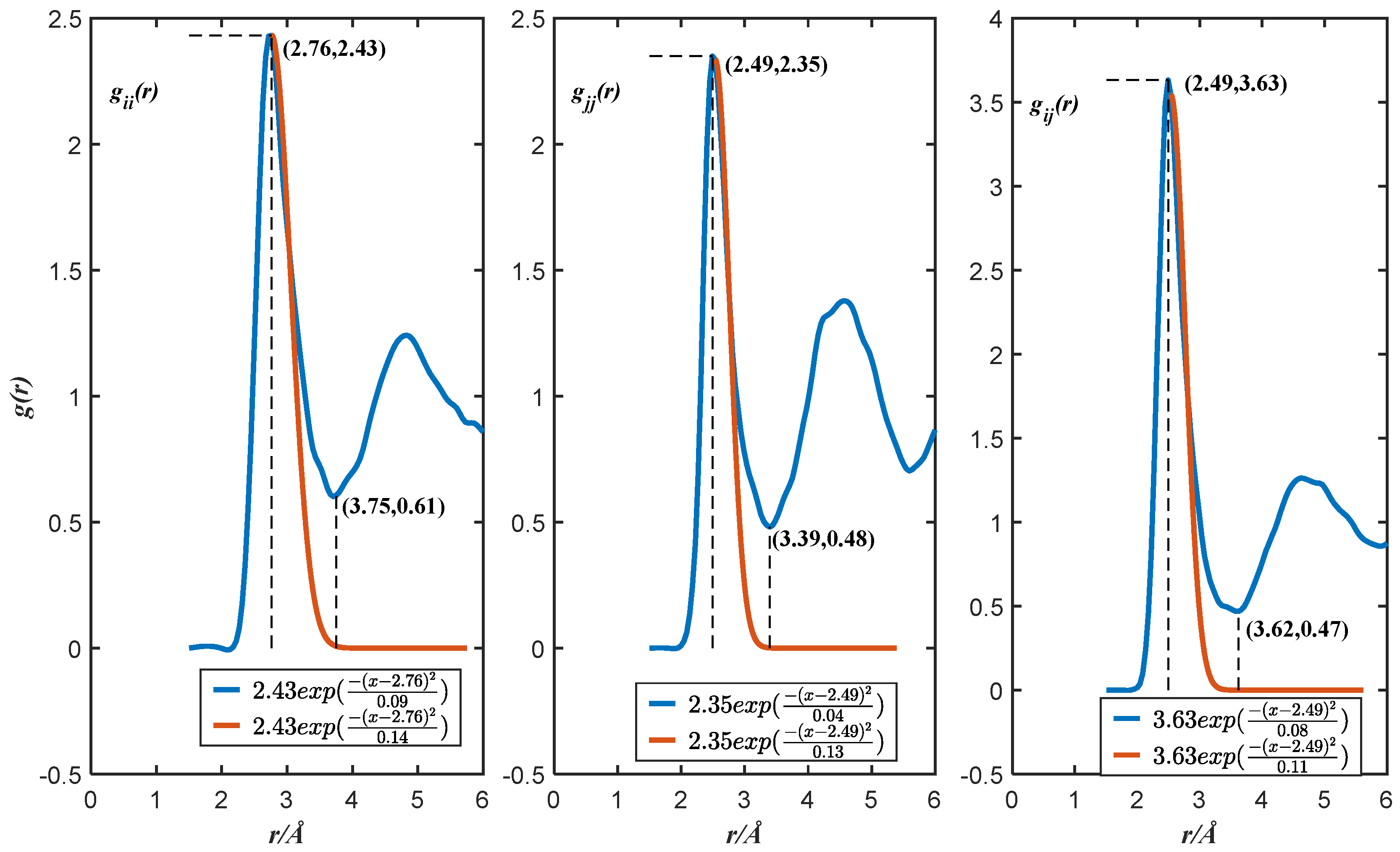
To clearly explain the method of combining PPDF and the thermodynamic model for estimations, Al0.6Cu0.4 was used as an example to estimate excess Gibbs free energy and activity. The corresponding L-PPDF mathematical expression was obtained according to Equation (1) [50], Equation (35) is the corresponding mathematical equation, Figure 2 is the L-PPDF function graph, and Table 1 lists the structural parameter tables.
g i i ( r ) = 2.43 exp 2.76 r 2 0.09 2.43 exp r 2.76 2 0.14 ; g j j ( r ) = 2.35 exp 2.41 r 2 0.04 2.35 exp r 2.41 2 0.13 ; g i j ( r ) = 3.63 exp 2.49 r 2 0.08 r < r m 3.63 exp r 2.49 2 0.11 r m < r
By substituting the data in Table 1 into Equations (8) and (9), the corresponding partial coordination numbers and pair potentials can be obtained. According to the model parameter equation, the specific model parameter values can be obtained. All model parameter values are listed in Table 2.
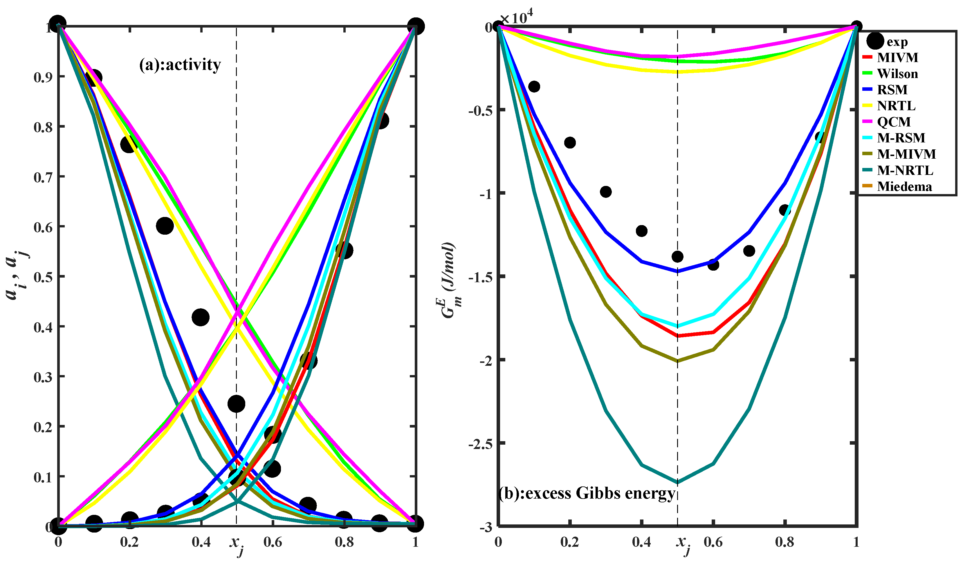
Substituting the model parameters in Table 2 into Equations (14), (17), (19), (21), (22), (25), (27), (28), and (33), the estimated values of molar excess Gibbs energy and activity by the eight equations can be achieved and compared with experiment data of the liquid Al-Cu at T = 1400 K [69], as shown in Figure 3
Analyzing Figure 3, it can be seen that the molar excess Gibbs energy of Al-Cu is a negative deviation system, which is not symmetric, about xj = 0.5, and the activity exhibits a deviation characteristic of moderate strength. All models are able to correctly describe the type of deviation of the molar excess Gibbs energy of Al-Cu, which is the most basic requirement for the reliability of the prediction methods. All models of molar excess Gibbs energy seem to be symmetric with xj = 0.5 and do not have a description of the asymmetric character of molar excess Gibbs energy. The difference between the models is the difference in the intensity of the deviations. The accuracies of the eight models describing molar excess Gibbs energy from good to bad are: RSM, M-RSM, MIVM, M-MIVM, M-NRTL, NRTL, Wilson, and QCM. The models can be divided into two classes; the absolute values of molar excess Gibbs free energy of Wilson, NRTL, and QCM are smaller than the experimental values, and the absolute values of molar excess Gibbs free energy of RSM, M-RSM, MIVM, M-MIVM, and M-NRTL are larger than the experimental values. RSM is based on cell theories and is the best performer, and the main problem of RSM is that it is not adapted to asymmetric systems. M-RSM is strongly correlated with RSM, and the difference between the two equations is that the molecular pair statistics methods are different, but M-RSM inherits the main information of RSM, so M-RSM also performs better. The relationship between M-RSM and M-MIVM can be described by the formula: M-MIVM = M-RSM + Wilson. It is known that the molar excess Gibbs energy description given by Wilson is significantly small, and in M-MIVM, M-RSM plays a dominant role. Furthermore, due to the strong correlation between MIVM and M-MIVM, it can be deduced that the main role in MIVM is enthalpy term (energy term). It can be concluded that the suitability of Al-Cu on cell theories is the main reason for the good performance of RSM, M-RSM, MIVM, and M-MIVM. The reason for the poor performance of Wilson and NRTL can be attributed to the theoretical basis of the model, which is based on local structure theory and does not fully match the theoretical basis of the distribution function. The QCM and RSM are more alike and their poor performance is probably related to the calculation methods of the parameters. M-NRTL adds the coordination number based on NRTL, and it is not straightforward to know which one performs better, so quantitative analysis needs to be done. By applying the ARD Equation (36), the ARD values can be obtained and are listed in Table 3. The ARD of molar excess Gibbs energy and activity of NRTL are 84.67% and 459.87%, respectively, and the ARD of M-NRTL are 65.61% and 47.56%, respectively. Adding the coordination number to NRTL indeed has the effect of improving the model performance. The preliminary conclusion that we can obtain with the Al-Cu analysis is that the theoretical basis of the model is important for estimating performance. The method of calculation of model parameters affects the performance of the model.
± A R D % = 100 % N n = 1 N G m E exp n G m E c a l n G m E exp n ± A R D % = 100 % 2 N n = 1 N a i exp n a i cal n a i exp n + a j exp n a j cal n a j exp n

3.2. Estimating Thermodynamic Values

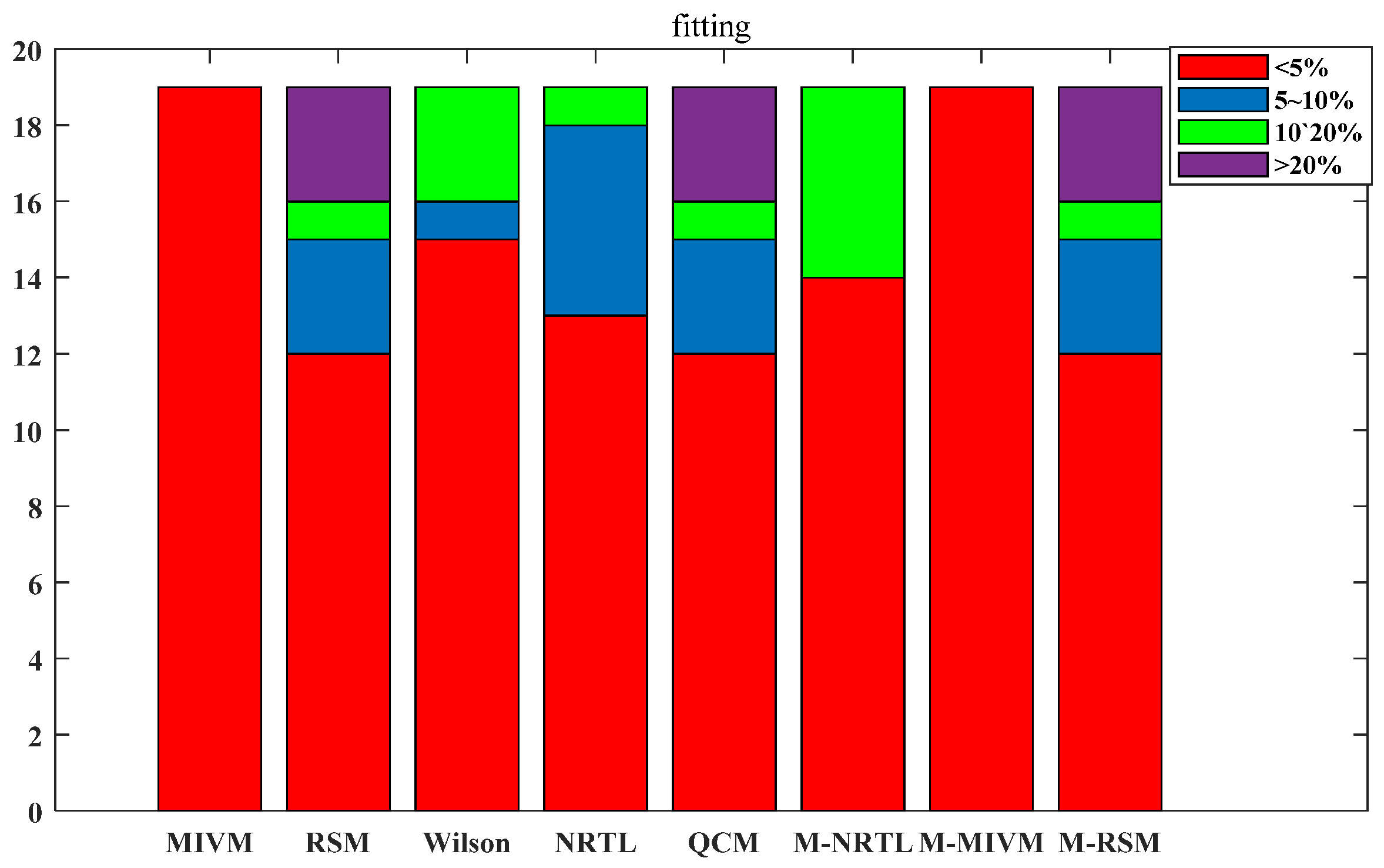
The descriptive capability of the model will be limited by its theoretical basis, and the adaptability of the model can be expressed by fitting. If the model has a poor fitting performance, it will naturally not have a satisfactory estimation performance. If the model has a poor fit performance, it cannot have a good estimation performance. Fitting analysis was conducted for the eight models, the ARD of the activities are shown in Figure 4. MIVM and M-MIVM showed superior performance in all 19 liquid alloys. The bar graphs of RSM, M-RSM, and QCM were consistent. This is because RSM, M-RSM, and QCM have different definitions of parameters, but when used for fitting, they are all essentially single-parameter models, thus exhibiting the same fitting performance. RSM, M-RSM, and QCM had three alloys with an ARD greater than ±20%: Al-Au: ±39.08%; Al-Cu: ±30.88%; Cu-Sb: ±24.94%. Their estimation performance was poor. When evaluating the estimative capabilities of the three models, the aforementioned three alloys should be excluded. NRTL, Wilson, and M-NRTL are two-parameter models, and they demonstrate well-fitting performances in most alloys with an ARD of less than ±20%, allowing for a reasonable description of the activity of all systems. The strength of the model fitting ability and the number of adjustable parameters were significantly correlated. The order of the fitting ability of the eight models was MIVM = M-MIVM > NRTL > Wilson > M-NRTL > RSM = M-RSM = QCM.
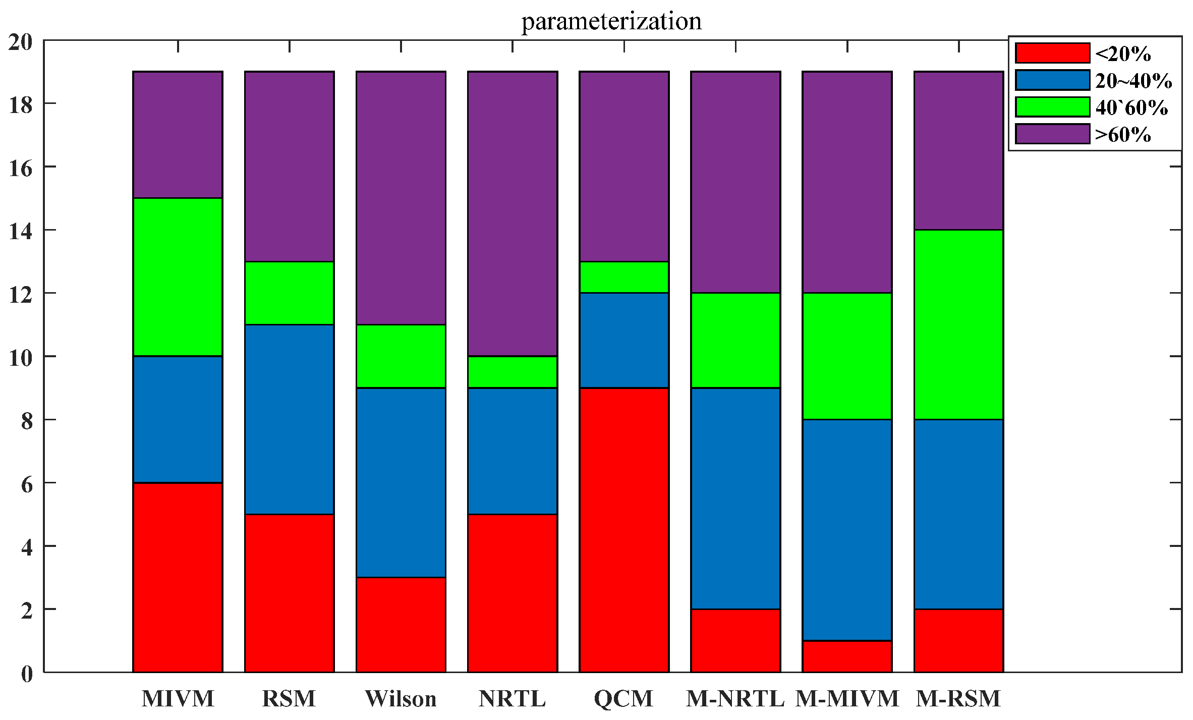
The data in Table S42 in the Supplemental Material were used to derive a first-order linear function of the parameters of components, which was then used to estimate the molar excess Gibbs energy and activity of each alloy using each model. The ARD of activity is visualized in Figure 5. After the parameters were expressed as functions, overall, the proportion of all models with an ARD < ±20% was relatively low, indicating that the model estimation performance was poor. Apart from the QCM, the other seven models had an ARD > ±40% for half of the alloys. This may indicate that obtaining the model parameters as a function of components was not advantageous in this work. The QCM performed better than other models because Dorini’s method uses multiple L-PPDFs for fitting and expresses Z and β as a function of the components. The other seven models introduced local structural parameters by solving the equations for the model parameters, which may be affected by fluctuations in the PDDF. If the model parameters were expressed as a function of the components, the fluctuations of the parameters could easily exceed the permissible limits of the model. The issue is that the variations in PPDF with components are objective, and the parameters should be dependent on the components. However, experience has demonstrated that expressing the model parameters as a linear function of composition is inadequate. In theory, to achieve a high-precision estimation, the model parameters should be represented as a function of components, which must be solved in subsequent research.
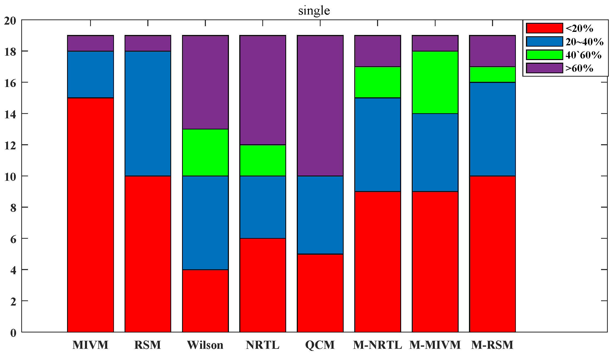
The parameters in Table S41 in the Supplemental Material were put into the model to estimate and evaluate the model’s performance when the parameter constants were manipulated. The ARDs with the best single-component estimation performance are shown in Figure 6, and the ARD with the average of the parameter values are shown in Figure 7. By analyzing Figure 6, it can be seen that MIVM achieved an ARD of less than ±20% for 15 alloys, indicating good performance. RSM and M-RSM achieved an ARD of less than ±20% for 10 alloys. M-NRTL and M-MIVM obtained an ARD of less than ±20% for nine alloys. Wilson, NRTL, and QCM estimations performed poorly, with only four, six, and five alloys having an ARD of less than ±20%, respectively. MIVM, RSM, M-NRTL, M-MIVM, and M-RSM had good estimating performance, all with a common high number of alloys with an ARD of less than ±20%, and a low proportion of alloys with an ARD greater than ±40%. The significant difference between Figure 5 and Figure 6 further confirms that representing the parameters of the above models as component functions drastically reduces the model’s estimative ability. The poor performance of the Wilson, NRTL, and QCM models is highlighted by the high proportion of alloys with an ARD greater than ±40%, indicating that the combinations of L-PPDF and these three models are still not mature enough. M-NRTL was originally an improved model of NRTL in practice. A comparison of the results of NRTL and M-NRTL revealed that the reasonableness of the model itself has an influence on the performance of the model parameters calculated using L-PPDF. Analyzing Figure 5, it shows that QCM has better estimative performance, making it reasonable to use multiple L-PPDFs and fitting regression to calculate the model parameters for QCM. However, the method of solving the model parameters by solving equations is unsuitable, indicating that the representation of parameters can also influence the estimative performance of the model.
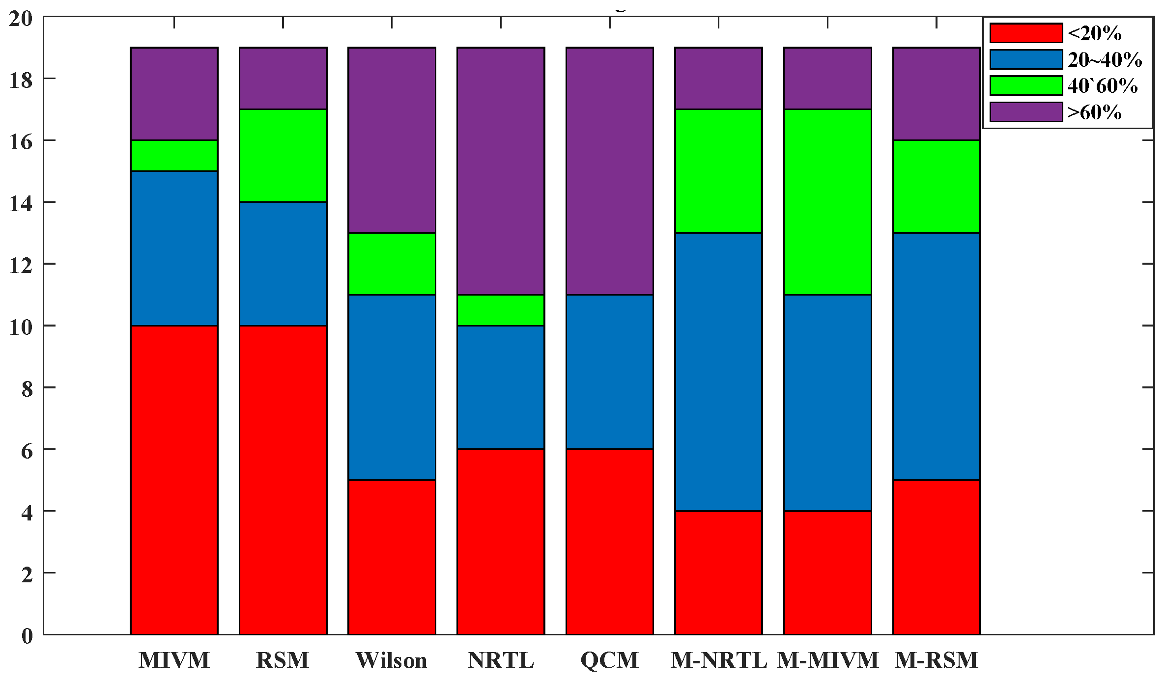
Figure 6 reflects the best model estimation performance, which is used to analyze the feasibility of L-PPDF combined with a thermodynamic model to estimate the excess Gibbs energy and activity. The purpose of parameter averaging is to demonstrate the average performance that an estimation made with parameters that any one component may have, which is more indicative of a model’s true estimative capability. Figure 7 shows the estimated ARD of the estimation graph corresponding to the average of the model parameters, which was significantly worse than in Figure 6. RSM and MIVM have good estimative performance, with an ARD of less than ±20% for 10 alloys. The corresponding numbers of alloys with an ARD less than ±20% for the Wilson, NRTL, QCM, M-NRTL, M-MIVM, and M-RSM were five, six, six, four, four, and five, respectively. The performance of MIVM, M-NRTL, M-MIVM, and M-RSM fluctuated greatly in Figure 6 and Figure 7, and the estimative performance of the four models decreased significantly after parameter averaging treatment. RSM, Wilson, NRTL, and QCM showed little variation in Figure 6 and Figure 7. After averaging MIVM model parameters, the estimation performance decreased, but half of the alloys still had an ARD of less than ±20%. The number of alloys with an ARD greater than 40% increased from one to four. The theoretical basis of the MIVM model is superior to that of the RSM, so naturally, it will perform better than the RSM in the optimal situation. In Figure 7, the performance of MIVM and RSM were similar, which is due to their common local structure theoretical basis. Compared with the other models, RSM showed better adaptability to parameter fluctuations, which made it suitable for treating parameters as constants. Thus, it can be expected that RSM will show similar performance when estimating with any set of L-PPDFs. The estimation performance of RSM is more dependent on the applicability of its model in the system. RSM is a strict regular solution model that is unsuitable for describing the energy changes caused by volume changes during liquid mixing processes. Consequently, RSM cannot accurately describe systems with asymmetric activity curves and mixing deviations, which limits its performance for such systems. Wilson, NRTL, and QCM used parameter averages with half the number of alloys having an ARD greater than ±60%, showing that these three models had poor estimation performance. A total of three models, M-MIVM, M-RSM, and M-NRTL, showed similar estimation performance. The significant features of the three models were that there were few alloys with an ARD of less than ±20% and greater than 60%. Most alloys had an ARD in the range of ±20 to ±40%. For these three models, the parameters are averages, and only reasonable estimations of low-precision estimates can be obtained.

4. Conclusions

In this work, the parameters of the MIVM, RSM, Wilson’s model, NRTL model, and QCM models were calculated using L-PPDF to estimate the excess Gibbs energy and activity of 19 alloys. MIVM achieved an ARD less than ±20% for 15 alloys; RSM had an ARD of less than ±20% for 10 alloys; QCM achieved an ARD of less than ±20% for nine alloys; NRTL itself had poor estimation performance, but upon increasing the coordination numbers, M-NRTL achieved an ARD of less than ±20% for 10 alloys. Based on an understanding of the local structure of a mixture, the representation of the neighboring molecular pairs in the derivation process of MIVM and RSM was changed to obtain two new model forms: M-MIVM and M-RSM. These achieved an ARD of less than ±20% for nine and eight alloys, respectively. Of the models mentioned in this paper, only Wilson’s estimation performance was always poor, with an ARD of less than ±20% for only five alloys. The experimental results show that the method proposed in this work for calculating the thermodynamic model parameters using L-PPDF to estimate the activity of mixtures is feasible and has a certain range of applicability.
The reliability of the method of combining PPDF and thermodynamic models to achieve molar excess Gibbs energy and activity estimation is demonstrated by statistical results for 19 liquid alloys. To prove the reliability of the approach, it needs to be validated in a larger number of systems. The present work does not analyze the PPDF-thermodynamic model performance differences in different types of liquid alloys. The performance of the method can be improved by studying the applicability of the PPDF-thermodynamic model in different systems. The L-PPDF representation of the potential function used in this work is simple and does not represent the true potential distribution of a liquid system. There are many studies on the calculation of the potential function using the distribution function, which can be combined with the method proposed in this work to improve the PPDF-thermodynamic model performance. In general, the PPDF-thermodynamic model for estimating the molar excess Gibbs energy and activity has a large potential, and with continued intensive research, the method has the potential to achieve an accuracy consistent with experimentally determined thermodynamic data.

Supplementary Materials

The following supporting information can be downloaded at: https://www.mdpi.com/article/10.3390/met13050996/s1, Figures S1–S19: The partial pair distribution function for 19 alloys; Figure S20–S38: The activity and molar excess Gibbs energy of the 19 alloys for eight equations; Figures S39–S42 depict the plots of w/ZkT and Z with xi for the nineteen alloys; Figures S43–S46 show the variations in the four model parameters, Bij, Bji, λij and λji with xi; Figures S47–S50 show the variation of the two model parameters, ψij and ψji with xi.; Tables S1–S19: The equation parameter of local partial distribution function gii(r), gjj(r), gij(r) of 19 alloys ; Tables S20–S38: The models parameters solved by local partial pair distribution function under the multiple mole fractions of 19 alloys; Tables S39–S40: Fitting parameters of eight models in nineteen alloys; Table S41 The constant model parameters for 19 alloys. Table S42 The coefficients of the first-order equation for the model parameters of 19 alloys. Tables S43–S46: The eight models applying four methods of calculating parameters to obtain the average relative deviation of Gibbs excess free energy and activity for 19 alloys; The MMIVM derivation process. The M-RSM derivation process.

Author Contributions

D.T. and X.C. conceived the idea of modifying the empirical equations of local coordination numbers and molecular interaction volume model (MIVM) by partial radial distribution function (PPDF) for estimating component activities and molar excess Gibbs energy of binary liquid alloys, and guided the paper writing. C.W. modified the models, calculated model parameters and estimated component activities and molar excess Gibbs energy of 19 binary liquid alloys by their PPDF in the literatures; wrote the paper. All authors have read and agreed to the published version of the manuscript.

Funding

This work was financially supported by the National Natural Science Foundation of China under Grant (Grant No. 51464022).

Data Availability Statement

Data available on request from the authors.

Conflicts of Interest

On behalf of all authors, the corresponding author states that there is no conflict of interest.

Nomenclature

Aij, AjiWilson’s model parameters
Bij, Bji, λij, λjimolecular interaction volume model (MIVM) parameters
Ψij,Ψjimodify molecular interaction volume model (MIVM) and modify regular solution model parameters
G m E molar excess Gibbs energy, J/mol
Pii(r), Pjj(r), Pij(r)probability density function of pairs i-i, j-j, i-j
Rgas constant, 8.314 J/(K·mol)
Tabsolute temperature, K
Vmi,Vmjmolar volume of i and j, cm3/mol
Zii, Zjj, Zij, Zjjlocal coordination number (the first subscript represents the central atom; the second subscript represents the surrounding atom)
Zi, Zjthe first coordination number of i and j
Z average coordination number of liquid alloy
Z0, Zcthe parameters in the first-order multinomial expression of Z
ai, ajactivity of component i and j
gii(r), gjj(r), gij(r), gji(r)local partial pair distribution functions. gij(r) is the probability of finding atom j in the spherical shell in the interval r to r + dr centered on atom i. gii(r), gjj(r) and gji(r) have similar meanings.
r0position of the starting coordinate of pair distribution function is not 0, Å
rmposition of the first peak of the partial pair distribution function, Å
r1coordinate of the valley of the partial pair distribution function, Å
kBoltzmann constant, 1.38 × 10⁻²³ J/K
xii, xij, xjj, xjilocal molecular fractions
xi, xjmolar fractions of i and j
u, vGaussian function width parameter
Wregular solution model parameter
εii(r), εjj(r), εij(r), εjj(r)local pair potential function, J
εii, εij, εij, εjjmolecular pair potential, J
ω, βquasi chemical model parameters
σshort-range ordering
τij, τji, αijnonrandom two-liquid model parameters
ρ0average number density Å−3
γi, γjactivity coefficient of i, j
P1, P2parameters of the first order linear equation
AIMDab initio molecular dynamics
ARDaverage relative deviation
MIVMmolecular interaction volume model
M-MIVMmodify molecular interaction volume model
M-RSMmodify regular solution model
NRTLnonrandom two-liquid
PPDFpartial pair distribution function
L-PPDFlocal partial pair distribution function
QCMquasi-chemical model
UNIQUACuniversal quasi-chemical theory
RSMregular solution model
STGEScientific Group Thermodata Group Europe

References

  1. Su, Y.; Duan, S.C.; Guo, H.J.; Guo, J. Thermodynamic Properties Prediction of Fe-Al-Ti Alloys Based on Atom and Molecule Coexistence Theory. Phys. Met. Metallogr. 2022, 123, 1287–1298. [Google Scholar] [CrossRef]
  2. Islam, M.R.; Tanveer, S.; Chen, C.C. Modeling swelling behavior of hydrogels in aqueous organic solvents. Chem. Eng. Sci. 2021, 242, 116744. [Google Scholar] [CrossRef]
  3. Mounir, A.; Messnaoui, B.; Dinane, A.; Samaouali, A. New thermodynamic data for KNO3-sucrose-water ternary system: Water activity, osmotic coefficient, activity coefficient, excess Gibbs energy, solubility and transfer Gibbs energy at 298.15 K. Fluid Phase Equilib. 2020, 506, 112399. [Google Scholar] [CrossRef]
  4. Ha, C.; Kim, Y.M.; Woo, S.K.; Maawad, E.; Letzig, D.; Yi, S. Analysis of the dislocation activity of Mg-Zn-Y alloy using synchrotron radiation under tensile loading. J. Synchrotron Radiat. 2023, 30, 1–7. [Google Scholar] [CrossRef]
  5. Zhang, M.; Zhu, Z.Y.; Zhang, L.S.; Gao, M.R.; Gao, J.; Du, M.K.; Wang, B.Y. Understanding microstructure evolution and corrosion behavior of wire arc cladding inconel 625 Superalloy by thermodynamic approaches. J. Alloys Compd. 2023, 947, 169530. [Google Scholar] [CrossRef]
  6. Chen, L.L.; Li, T.; Zhang, J.P.; Wang, Y.A.; Kong, L.X.; Xu, B.Q.; Yang, B.; Wu, M.Z. Modeling and measurement of vapor-liquid equilibrium of In-Pb and In-Pb-Sn alloy systems in vacuum distillation. Vacuum 2023, 207, 111556. [Google Scholar] [CrossRef]
  7. Zhu, Y.Q.; Chen, Z.J.; Zhang, H.M.; Ma, W.H.; Wu, J.J. The effect of Ni on Fe and Al impurities by MIVM model for the silicon production. Energy 2022, 254, 124459. [Google Scholar] [CrossRef]
  8. Wang, S.L.; Hou, K.; Zhang, Z.W.; Huang, S.X.; Liu, X.Y.; He, M.G. Vapor-liquid equilibrium for dimethyl ether and three imidazolium ionic liquids as working pairs in absorption-refrigeration cycle. J. Mol. Liq. 2023, 380, 121742. [Google Scholar] [CrossRef]
  9. Xue, Q.; Kang, R.; Klionsky, D.J.; Tang, D.L.; Liu, J.B.; Chen, X. Copper metabolism in cell death and autophagy. Autophagy, 2023; just accepted. [Google Scholar]
  10. Wang, S.P.; Chen, L.L.; Xu, B.Q.; Jiang, W.L.; Kong, L.X.; Yang, B.; Xiong, H.; Qu, C.; Zhang, T.; Zhang, S.H.; et al. Theoretical calculation and experimental investigation on vacuum gasification separation of Ag-Cu-Au ternary alloy. J. Alloys Compd. 2023, 948, 169685. [Google Scholar] [CrossRef]
  11. El Guendouzi, M.; Benbiyi, A.; Dinane, A.; Azougen, R. Determination of water activities and osmotic and activity coefficients of the system NaCl-BaCl2-H2O at 298.15 K. Calphad 2003, 27, 375–381. [Google Scholar] [CrossRef]
  12. Hu, J.X.; Peng, D.L.; Huang, X.Y.; Wang, N.L.; Liu, B.Q.; Di, D.L.; Liu, J.F.; Qu, Q.L.; Pei, D. COSMO-SAC and QSPR combined models: A flexible and reliable strategy for screening the extraction efficiency of deep eutectic solvents. Sep. Purif. Technol. 2023, 315, 123699. [Google Scholar] [CrossRef]
  13. Zhao, X.; Cheng, S.X.; Koh, Y.P.; Kelly, B.D.; McKenna, G.B.; Simon, S.L. Prediction of the Synergistic Glass Transition Temperature of Coamorphous Molecular Glasses Using Activity Coefficient Models. Mol. Pharmaceut. 2021, 18, 3439–3451. [Google Scholar] [CrossRef] [PubMed]
  14. Sum, A.K.; Sandler, S.I. Use of ab initio methods to make phase equilibria predictions using activity coefficient models. Fluid Phase Equilib. 1999, 158, 375–380. [Google Scholar] [CrossRef]
  15. Wilson, G.M. Vapor-Liquid Equilibrium. XI. A New Expression for the Excess Free Energy of Mixing. J. Am. Chem. Soc. 1963, 86, 127–130. [Google Scholar] [CrossRef]
  16. Raabe, G.; Koehler, J. Use of ab initio interaction energies for the prediction of phase equilibria in the system nitrogen-ethane. Phys. Chem. Chem. Phys. 2002, 6, 926–930. [Google Scholar] [CrossRef]
  17. Neiman, M.; Cheng, H.; Parekh, V. A critical assessment on two predictive models of binary vapor liquid equilibrium. Phys. Chem. Chem. Phys. 2004, 13, 3474–3483. [Google Scholar] [CrossRef]
  18. Haghtalab, A.; Yousefi, J.S. A new insight to validation of local composition models in binary mixtures using molecular dynamic simulation. AIChE J. 2015, 1, 275–286. [Google Scholar] [CrossRef]
  19. Ravichandran, A.; Khare, R.; Chen, C.C. Predicting NRTL binary interaction parameters from molecular simulations. AIChE J. 2018, 64, 2758–2769. [Google Scholar] [CrossRef]
  20. Ravichandran, A.; Tun, H.; Khare, R.; Chen, C.C. Prediction of thermodynamic properties of organic mixtures: Combining molecular simulations with classical thermodynamics. Fluid Phase Equilib. 2020, 523, 1–10. [Google Scholar] [CrossRef]
  21. Dorini, T.T.; Eleno, L. Liquid Bi–Pb; Bi–Li alloys: Mining thermodynamic properties from ab-initio molecular dynamics calculations using thermodynamic models. Calphad 2019, 67, 101687. [Google Scholar] [CrossRef]
  22. Guggenheim, E.A. Statistical thermodynamics of co-operative systems (a generalization of the quasi-chemical method). Trans. Faraday Soc. 1948, 44, 263–271. [Google Scholar] [CrossRef]
  23. Tao, D.P. A new model of thermodynamics of liquid mixtures and its application to liquid alloys. Thermochim. Acta 2000, 363, 105–113. [Google Scholar] [CrossRef]
  24. Hildebrand, J.H. Solubility. XII. regular solutions. J. Am. Chem. Soc. 1929, 51, 66–80. [Google Scholar] [CrossRef]
  25. Renon, H.; Prausnitz, J.M. Local Composition Thermodynamic Excess Functions for Liquid Mixtures. AIChE J. 1968, 14, 135–144. [Google Scholar] [CrossRef]
  26. Zernike, F.; Prins, J.A. Die Beugung von Röntgenstrahlen in Flüssigkeiten als Effekt der Molekülanordnung. Z. Phys. A Hadron. Nucl. 1927, 41, 184–194. [Google Scholar] [CrossRef]
  27. Acree, W.E. Comments on excess molar volumes reported in “Study of short range and long range molecular interactions in binary liquid mixtures of N,N—dimethylformamide (DMF) and 1-propanol”. J Mol. Liq. 2022, 360, 118832. [Google Scholar] [CrossRef]
  28. Mokshin, A.V.; Khusnutdinoff, R.M.; Galimzyanov, B.N.; Brazhkin, V.V. Extended Short-Range Order Determines the Overall Structure of Liquid Gallium. Phys. Chem. Chem. Phys. 2020, 22, 4122–4129. [Google Scholar] [CrossRef]
  29. Roik, O.S.; Yakovenko, O.M.; Kashirina, Y.O.; Kazimirov, V.P.; Sokol’Skii, V.E.; Rebenko, M.Y.; Galushko, S.M.; Golovataya, N.V. The short-range order in liquid Al-Co-Sn alloys. Phys. Chem. Liq. 2022, 60, 625–635. [Google Scholar] [CrossRef]
  30. Wang, C.; Chen, X.; Tao, D. Development of a Non-Integral Form of Coordination Number Equation Based on Pair Distribution Function; Gaussian Function. Metals 2023, 13, 384. [Google Scholar] [CrossRef]
  31. Khambholja, S.G.; Abhishek, A. Structure factor and radial distribution function of liquid Pb83Li17. DAE Solid State Phys. Symp. 2019, 2020, 030365. [Google Scholar] [CrossRef]
  32. Su, Y.; Wang, X.D.; Cao, Q.P.; Zhang, D.X.; Jiang, J.Z. Different Thermal Responses of Local Structures in Pd43Cu27Ni10P20 Alloy from Glass to Liquid. J. Phys. Chem. C 2020, 124, 19817–19828. [Google Scholar] [CrossRef]
  33. Waseda, Y. The Structure of Non-Crystalline Materials: Liquids and Amorphous Solids; McGraw-Hill International Book: New York, NY, USA, 1980; pp. 47–49. [Google Scholar]
  34. Mikolaj, P.G.; Pings, C.J. The Use of the Coordination Number in the Interpretation of Fluid Structure. Phys. Chem. Liq. 1968, 1, 93–108. [Google Scholar] [CrossRef]
  35. Cahoon, J.R. The first coordination number for liquid metals. Can. J. Phys. 2004, 82, 291–301. [Google Scholar] [CrossRef]
  36. Liu, J.H.; Zhang, L. Structural and Thermodynamic Behaviors of CumAgn (m + n = 144–147) Nanoalloys during Cooling: Implications for Nanoparticle Structure Control. ACS Appl. Nano Mater. 2023, 6, 6388–6397. [Google Scholar] [CrossRef]
  37. Gosh, R.C.; Pandit, A.; Sarkar, S. A comparative study on surface tension, diffusion coefficient and shear viscosity coefficient of liquid transition metals. J. Non-Cryst. Solids 2023, 606, 122176. [Google Scholar] [CrossRef]
  38. Davidson, N. Statistical Mechanics; Series in Advanced Chemistry; McGraw Hill: New York, NY, USA, 1962; pp. 474–475. [Google Scholar]
  39. Feller, W. An Introduction to Probability Theory and Its Applications; Wiley: Hoboken, NJ, USA, 1950; pp. 220–222. [Google Scholar]
  40. Iida, T.; Guthrie, R. The Physical Properties of Liquid Metals; Oxford University Press: Oxford, UK, 1988; pp. 71–72. [Google Scholar]
  41. Nakanishi, K.; Okazaki, S.; Ikari, K.; Higuchi, T.; Tanaka, H. Free Energy of Mixing, Phase Stability, and Local Composition in Lennard-Jones Liquid Mixtures. J. Chem. Phys. 1982, 76, 629–636. [Google Scholar] [CrossRef]
  42. Lennard-Jones, J.E.; Devonshire, A.F. Critical phenomena in gases-I. Proc. R. Soc. Ser. A Math. Phys. Eng. Sci. 1937, 163, 53–70. [Google Scholar]
  43. Guggenheim, E.A. Application of Statistical Mechanics; Oxford University Press: Oxford, UK, 1966; p. 211. [Google Scholar]
  44. Cheremisina, E.; Gao, X.; Ueda, S.; Kitamura, S.; Yamashina, R.; Schenk, J. Experimental Determination of the MnO Activity Coefficient in High-Manganese Slags Using the Chemical Equilibrium Method. Metals 2021, 11, 1190. [Google Scholar] [CrossRef]
  45. Sui, Y.R.; Ding, Z.X.; Zhai, C.; Lin, H.S.; Wu, W. Crystallization-free and low-cost deep eutectic solvents for absorption thermal battery utilizing ultra-low-grade energy. Energy Convers. Manag. 2023, 284, 116984. [Google Scholar] [CrossRef]
  46. Prausnitz, J.M.; Lichtenthaler, R.N.; Azevedo, E. Molecular Thermodynamics of Fluid-Phase Equilibria; Prentice-Hall: Hoboken, NJ, USA, 1999; p. 296. [Google Scholar]
  47. Tsilifis, P.; Browning, W.J.; Wood, T.E.; Newton, P.K.; Ghanem, R.G. The Stochastic Quasi-chemical Model for Bacterial Growth: Variational Bayesian Parameter Update. J. Nonlinear Sci. 2018, 28, 371–393. [Google Scholar] [CrossRef]
  48. Tao, D.P. The universal characteristics of a thermodynamic model to conform to the Gibbs-Duhem equation. Sci. Rep. 2016, 6, 35792. [Google Scholar] [CrossRef] [PubMed]
  49. Voigtmann, T.; Kolland, G.; Kobatake, H.; Brillo, J.; Peng, H.L. Structural and dynamical properties of liquid Al-Au alloys. Phys. Rev. B 2015, 92, 184–201. [Google Scholar]
  50. Roik, O.S.; Samsonnikov, O.V.; Kazimirov, V.P.; Sokolskii, V.E.; Galushko, S.M. Medium-range order in Al-based liquid binary alloys. J. Mol. Liq. 2010, 151, 42–49. [Google Scholar] [CrossRef]
  51. Kbirou, M.; Mazroui, M.; Hasnaoui, A. Atomic packing and fractal behavior of Al-Co metallic glasses. J. Alloys Compd. 2018, 735, 464–472. [Google Scholar] [CrossRef]
  52. Roik, O.S.; Yakovenko, O.M.; Kazimirov, V.P.; Bilovodska, O.O.; Sokolskii, V.E. RMC simulations of the liquid Al Ge alloys. J. Mol. Liq. 2016, 220, 155–160. [Google Scholar] [CrossRef]
  53. Faruk, M.M.; Bhuiyan, G.M. Investigation of segregation for Al-In liquid binary alloys. Phys. B Condens. Matter 2013, 422, 56–63. [Google Scholar] [CrossRef]
  54. Wang, C.C.; Wong, C.H. Short-to-medium range order of Al-Mg metallic glasses studied by molecular dynamics simulations. J. Alloys Compd. 2011, 509, 10222–10229. [Google Scholar] [CrossRef]
  55. Qin, J.; Pan, S.; Qi, Y.; Gu, T. The structure and thermodynamic properties of liquid Al-Si alloys by ab initio molecular dynamics simulation. J. Non-Cryst. Solids 2016, 433, 31–37. [Google Scholar] [CrossRef]
  56. Roik, O.S.; Yakovenko, O.M.; Kazimirov, V.P.; Sokolskii, V.E.; Golovataya, N.V.; Kashirina, Y.O. Structure of liquid AlSn alloys. J. Mol. Liq. 2021, 330, 115570. [Google Scholar] [CrossRef]
  57. Souto, J.; Alemany, M.M.G.; Gallego, L.J.; González, L.E.; González, D.J. Static structure, microscopic dynamics and electronic properties of the liquid Bi–Pb alloy. An ab initio molecular dynamics study. J. Nucl. Mater 2011, 411, 163–170. [Google Scholar] [CrossRef]
  58. Chen, S.; Ma, J.; Dai, Y.; Yang, J.; Zhang, J.; Dong, Q.; Han, Y.; Xing, H.; Sun, B. Atomic-scale simulations of the local structures of molten Ni1-xCox and Ni1-xFex. J. Non-Cryst. Solids 2018, 481, 470–478. [Google Scholar] [CrossRef]
  59. Korkmaz, S.D.; Korkmaz, Ş. A study for structure and inter-diffusion coefficient of liquid K1−x Cs x metal alloys. Phys. Chem. Liq. 2011, 49, 801–810. [Google Scholar] [CrossRef]
  60. Faruk, M.M.; Bhuiyan, G.M.; Biswas, A.; Hossain, M.S. Study of microscopic origin of segregation for Fe x Cu1x and CuxCo1-x liquid binary alloys. J. Chem. Phys. 2014, 140, 134505. [Google Scholar] [CrossRef] [PubMed]
  61. Liu, D.; Qin, J.Y.; Gu, T.K. The structure of liquid Mg-Cu binary alloys. J. Non-Cryst. Solids 2010, 356, 1587–1592. [Google Scholar] [CrossRef]
  62. Guo, F.; Tian, Y.; Qin, J.; Xu, R.; Sun, Y. Structure of liquid Cu-Sb alloys by ab initio molecular dynamics simulations, high temperature X-ray diffraction, and resistivity. J. Mater Sci. 2013, 48, 4438–4445. [Google Scholar] [CrossRef]
  63. Jakse, N.; Nguyen, T.; Pasturel, A. Local order and dynamic properties of liquid and undercooled CuxZr1-x alloys by ab initio molecular dynamics. J. Appl. Phys. 2013, 114, 425. [Google Scholar] [CrossRef]
  64. Korkmaz and Korkmaz, S.D. Structure and Inter-Diffusion Coefficients of Liquid NaxK1-x Alloys. J. Phase Equilibria Diffus. 2010, 31, 15–21. [Google Scholar] [CrossRef]
  65. Liu, D.; Zhu, X.; Qin, J.; Wang, A.; Duan, J.; Gu, T. First-Principles Study of Chemical and Topological Short-Range Orders in the Mg-Si Liquid Alloys. Metals 2016, 6, 78. [Google Scholar] [CrossRef]
  66. Liu, D.; Qin, J.; Zhu, X.M.; Duan, J.P.; Gu, T.; Wang, A.M. Correlation between local structures and glass forming ability of liquid MgX-Zn(1-x) alloys. J. Non-Cryst. Solids 2016, 447, 262–266. [Google Scholar] [CrossRef]
  67. Hardy, H.K. A “sub-regular” solution model and its application to some binary alloy systems. J. Acta Metall. 1953, 1, 202–209. [Google Scholar] [CrossRef]
  68. Flemr, V. A note on excess Gibbs energy equations based on local composition concept. Collect. Czechoslov. Chem. Commun. 1976, 41, 3347–3349. [Google Scholar] [CrossRef]
  69. Franke, P.; Neusch, D. Elements and Binary Systems from Ag-AI to Au-TI; Springer: Berlin/Heidelberg, Germany, 2002; pp. 139–142. [Google Scholar]
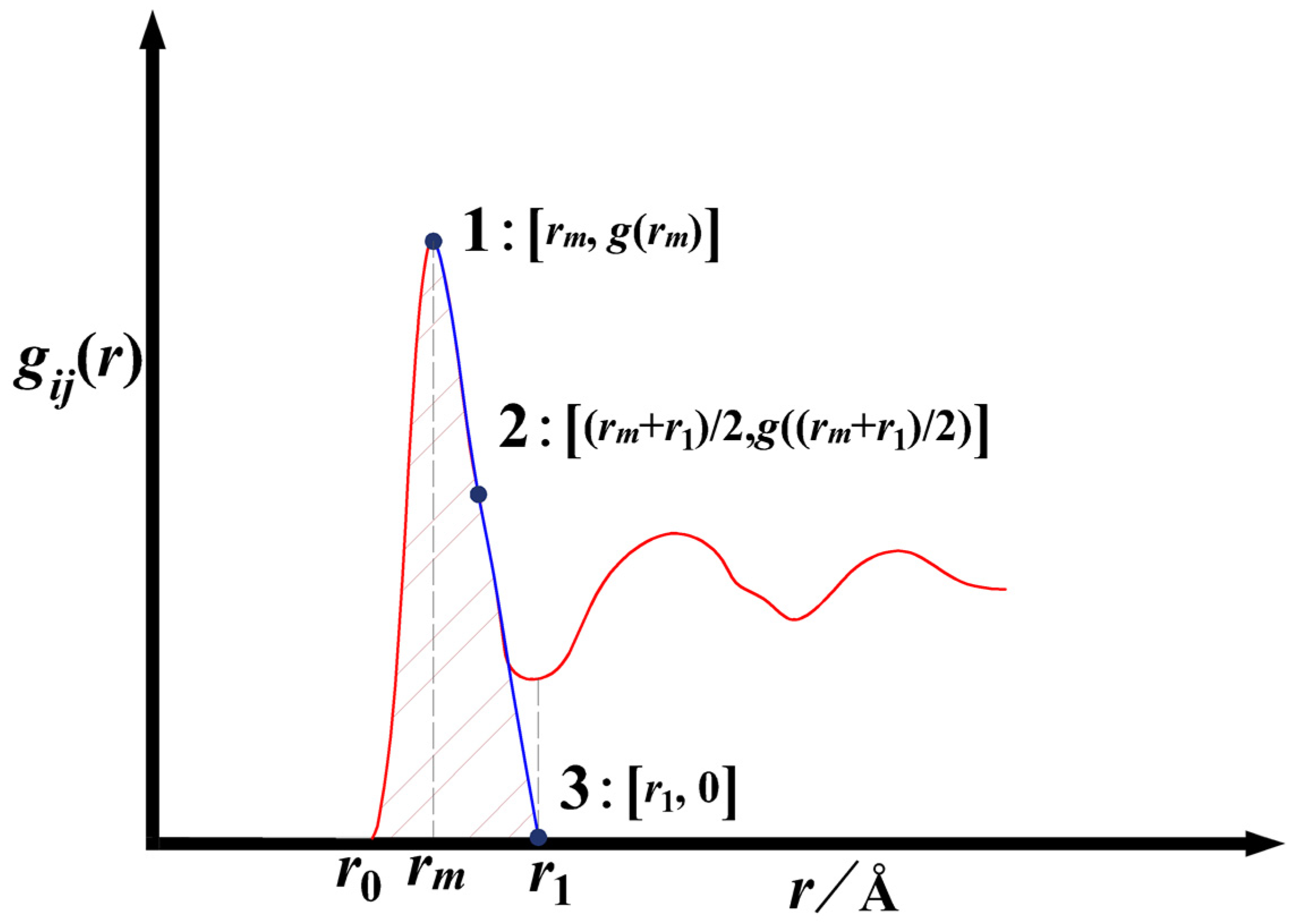
Figure 1. Schematic diagram of extracting the local partial pair distribution function (L-PPDF) from the partial pair distribution function (PPDF), 1 is (rm, g(rm)), 3 is (r1, 0), and 2 is ((rm + r1)/2, g((rm + r1)/2)), red curve is partial pair distribution function, blue curve is local partial pair distribution function.
Metals 13 00996 g001
Figure 2. The local partial pair distribution functions of Al0.6Cu0.4 alloy, T = 1400K [50].
Metals 13 00996 g002
Figure 3. Comparison of the estimated values of eight equations with experiment data (black dots) of activity and molar excess Gibbs energy of the liquid Al-Cu at T = 1400 K [69].
Metals 13 00996 g003
Figure 4. ARD comparison of the fitting of eight models for the activity of 19 alloys.
Metals 13 00996 g004
Figure 5. The parameters are expressed as functions after the ARD comparison of the estimated activity of the eight models in the 19 alloys.
Metals 13 00996 g005
Figure 6. ARD comparison of the estimations of activity in 19 alloys for eight models after taking the optimal single parameters.
Metals 13 00996 g006
Figure 7. ARD comparison of the estimated activities of 19 alloys using eight models after taking the average value of the parameters.
Metals 13 00996 g007
Table 1. The local structure parameters of Al0.6Cu0.4., T = 1400K.
Typeiijjij
r01.741.571.59
rm2.762.412.49
r14.674.233.85
g(rm)2.432.353.63
u0.210.140.19
v0.260.250.22
ρ00.0625xi0.6
r0,rm,r1, and g(rm) extracted from PPDF of Al0.6Cu0.4. [50], u, v obtained by fitting the L-PPDF.
Table 2. Model parameters of Al0.6Cu0.4., T = 1400 K.
Pair PotentialsPartial Coordination Numbers
εii/kTεij/kTεji/kTεjj/kTZiiZijZjiZjj
−0.37−0.745−0.75−0.315.323.785.682.26
MIVMRSMM-MIVM
BijBijλjiλjiZw/ZkTψijψji
1.660.430.430.388.63−0.865.383.67
QCM
σβω/ZkT
0.531.04−2.09
Table 3. The average relative deviations (ARD) of molar excess Gibbs energy and activity of the liquid Al-Cu at T = 1400 K for eight equations (±%).
ModelMIVMWilsonNRTLRSMQCMM-MIVMM-NRTLM-RSM
G m E 30.569.1565.6115.9972.2340.0784.6727.90
Activity28.40504.02459.8724.56605.1433.9947.5629.28
Disclaimer/Publisher’s Note: The statements, opinions and data contained in all publications are solely those of the individual author(s) and contributor(s) and not of MDPI and/or the editor(s). MDPI and/or the editor(s) disclaim responsibility for any injury to people or property resulting from any ideas, methods, instructions or products referred to in the content.