Development of a Non-Integral Form of Coordination Number Equation Based on Pair Distribution Function and Gaussian Function

Abstract

The coordination number (CN) is an important structure property of liquid metals. A simple yet extremely precise method for calculating CN is proposed, the classical CN methods are evaluated systematically, and the mathematical forms of the symmetry method are corrected. Using the Gaussian function construct, the first coordination shell of the pair distribution function (PDF), the right-hand side of the first peak of the pair distribution function is extrapolated, and the CN expression is simplified with a Gaussian function to obtain its non-integral form. The first coordination shell is used to explain the Tao coordination number model (Tao CN) and obtain a Modified Tao CN. The Gaussian function is combined with the Tao CN, obtaining the function expression for the peak with peak position. These are important for the structural research of liquid metals. The CN of 27 liquid metals is calculated by these methods. The average relative deviation of the Gaussian function extrapolation method is ±6.46%, of the Modified Tao CN is ± 18.51%; those of the four classical methods range from ±15% to ±42%. The Modified Tao CN and extrapolation methods to calculate CN are more accurate for calculating CN than the classical method; they are more suitable for use in quantitative applications of CN. The equations derived in this work can be applied to the problem of integration of distribution functions to obtain simple mathematical models.

1. Introduction

The coordination number (CN) is closely connected to the physical properties of liquid metal (diffusion coefficient [1], density, viscosity, etc. [2]); it is also the fundamental parameter of the excess Gibbs energy model based on a local structural theory (Wilson [3], MIVM [4,5]). CN is the area of the first coordination shell of the function 4πρ₀r²g(r). The g(r), pair distribution function (PDF), represents the probability density distribution of coordination shell atoms that interact with the central atom [6]. The first coordination shell of 4πρ₀r²g(r) needs to be obtained by g(r). Five classical determination methods are: (a) symmetrizing the first peak in g(r), obtaining g_a(r) [7]; (b) symmetrizing the first peak in 4πρ₀r²g(r), g_b(r) [8]; (c) symmetrizing the first peak in rg(r), g_c(r) [9]; (d) computing the area of 4πρ₀r²g(r) from zero to the first minimum position r_1, g_d(r); and (e) taking as the CN area the area under the first peak when the right-hand side of the first peak is extrapolated to the abscissa, g_e(r) [10]. Mikolaj calculated the CN of liquid argon in 13 states by methods b, c, d, and e; the results from methods b and c were less than the experimental value, while those of d and e were more than the experimental value [11]. Hong used methods c and d to calculate the CN of Hg, with results for method c of 6.0 and method d of 14.6 [12]. Vineyard used method b to calculate the CN of Hg, with a result for method b of 10.3 [13]. The CNs obtained by the various methods are quite different, making comparisons of the CN difficult. In addition to the above five common methods of constructing coordination shells, the method of constructing coordination shells is flexible. Higham gives the conditions under which atom i is centered and atom j is within its first coordination shell after molecular dynamic simulations have obtained the coordinate positions of the atoms and overcome the limitations of cutoffs for defining atomic coordination shells [14]. Srirangam investigated the use of the area under the first peak of the PDF curve reduced by subtracting the area under the extrapolated edge of the second peak [15,16]. Among the known methods for constructing the first coordination shell, method g_e(r) is more appropriate than the others. However, the specific construction methods for g_e(r) are not well defined, so practical application in research is rare. The method of constructing g_e(r) must be perfected to improve the accuracy of CN.

Besides calculating CN using g(r), researchers also constructed a model to determine CN without using g(r). Hines and Walls established a graph to reflect the relationship between the empty volume fraction and CN; the average relative deviations (ARDs) of the CNs calculated for 39 liquid metals was ±28.9% [17]. Cahoon estimated CN based on the CN-filling rate with a value range of 6.8–8.5, significantly smaller than experimental values [18]. Tao gives a model that requires only covalent diameter (d_cov), atomic diameter (σ), and average number density (ρ₀) to calculate CN. With the Tao CN method, the ARDs for 39 liquid metals are ±6.44% [19], thus significantly lower. Although the Tao CN performed well, the Tao CN derivation process was not rigorous. Tao assumes that the area of the first coordination shell has a normal distribution and ignores that the area of the normal distribution is a constant and the area of the first coordination shell is not a constant [20]. Tao, in using a constant value to replace an integration function, did not have a rigorous explanation. The Tao CN model needs further study before a fully supported explanation can be given.

Inaccurate values of coordination numbers can have an impact on the quantitative application of the prediction of thermodynamic properties [21,22]. This paper presents work that overcomes these limitations. Using PDFs of 27 liquid metals, for example, applies Gaussian functions to perfect the determination of g_e(r). First, the g_e(r) is improved by using the Gaussian function, which makes the extrapolation method more practical. Second, it applies the g_e(r) to explain the Tao CN and to give a rigorous Modified Tao CN that is more consistent with the theory behind g(r). In this process, the relationship between the peak position and the peak of g(r) is derived. Third, in analyzing classical CN calculation methods, the work points out the unreasonable descriptions of g_a(r) and g_c(r) as mathematical equations in the literature. Finally, the CNs of 27 liquid metals were calculated using the 3 CN equations given in this work and 4 of the classical CN equations, and the methods were systematically compared. The ARDs of the 27 liquid metals, Z_e is ±6.89%, and the Modified Tao CN is ±13.84%, both better than classical methods, with ARDs ranging from ±15.07% to ±32.85%. This detailed study of the methods of calculating CN of liquid metals has permitted the determination of a CN formulation with consistent, accurate results, providing a useful reference for the study of the CN of liquid metals.

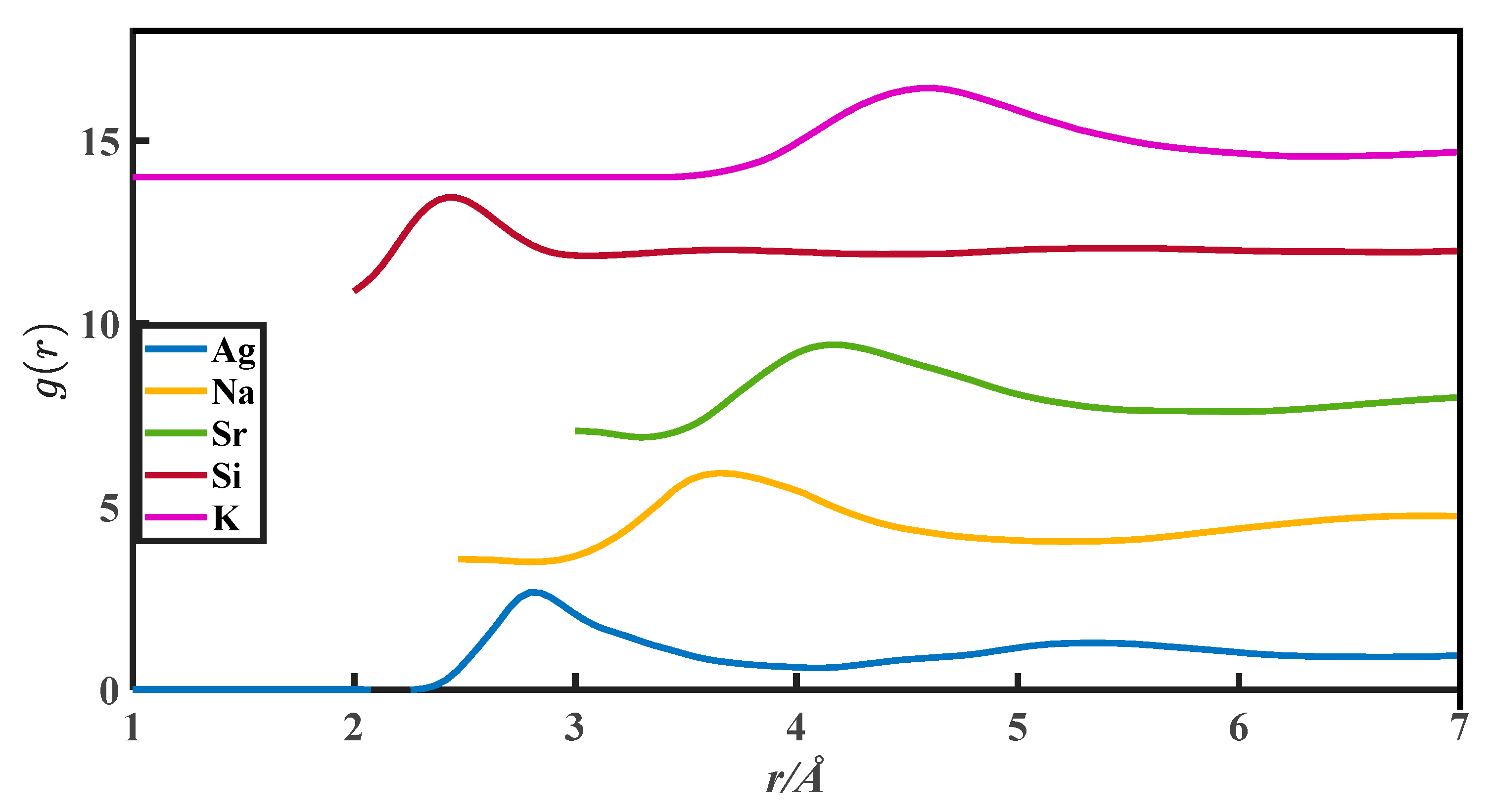
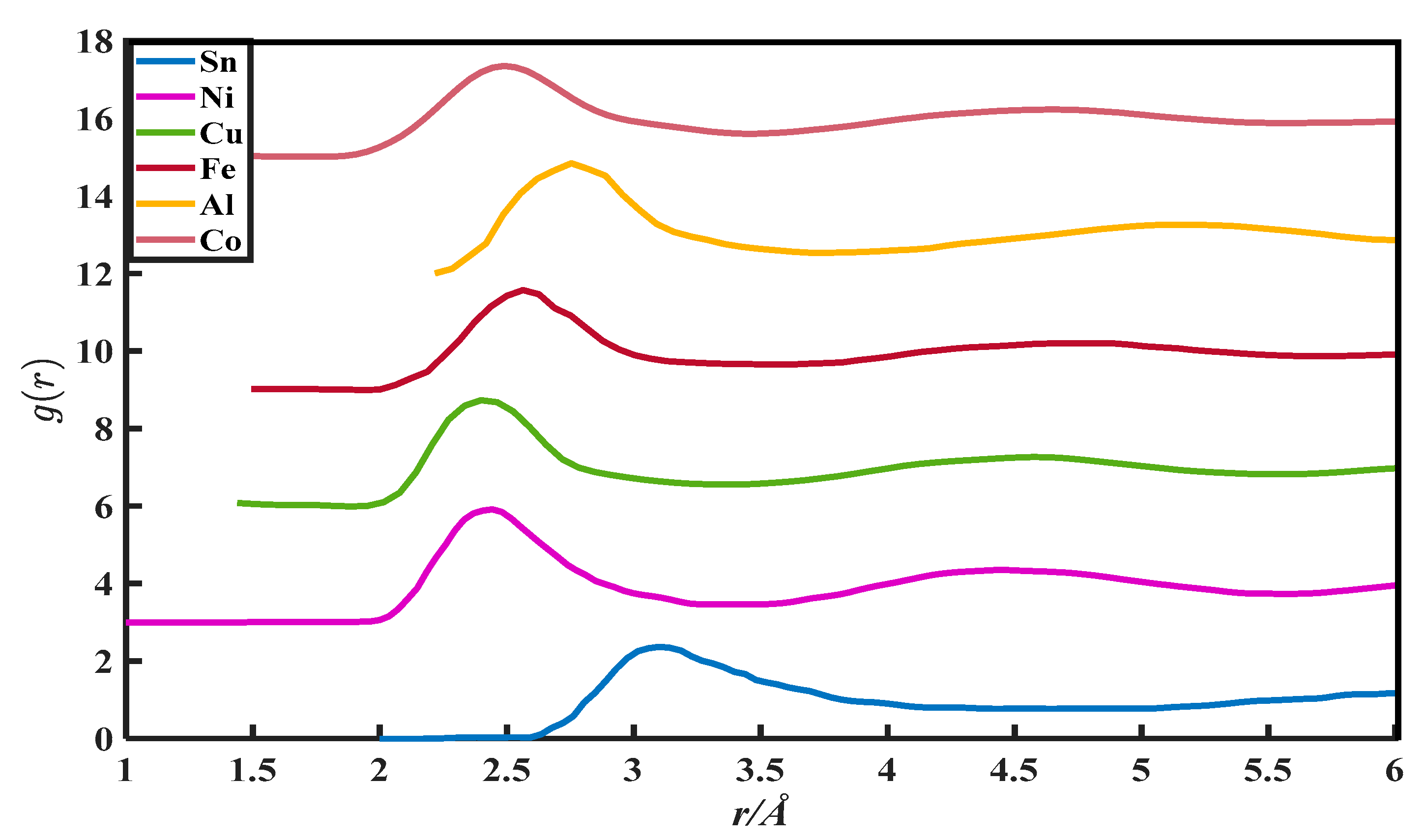
2. The g(r) Data

The CN calculation methods in this paper are all based on the PDFs, which are from Appendix 8 of The structure of Non-Crystalline Materials Liquid and Amorphous Solids [23]. The g(r) of 27 liquid metals is shown in Figure 1, Figure 2, Figure 3, Figure 4 and Figure 5.

3. Coordination Number Equation

This part introduces the Tao CN derivation process and points out the problem; the Gaussian functions used to construct the g_e(r) and the non-integral equation for CN are derived; g_e(r) is applied to explain the Tao CN and derive a function equation of r_m with g(r_m); and the classical methods are described, and the mathematical form of the g_a(r) and g_c(r) are modified. The CN methods in this section are all based on the CN definition as given in Equation (1) [6] (p. 21):

$$Z_{{}^i}={\displaystyle {\int }_{r_0}^{r_{\mathrm{end}}}4\pi r^2{\rho }_0{g}_i(r)dr}$$

(1)

where ρ₀ = N/V = 0.6022/V_m is the average number density; V_m is the molar volume; g_i(r) is the first coordination shell of different methods; Z_i is the CN of the different methods. The subscript i indicates the different method tags, which are a, b, c, d, and e, as described in the introduction. r₀ is the starting point of g(r), not 0, and all methods have the same r₀. r_end is the upper limit of integration of the function.

3.1. Tao Coordination Number Model (Tao CN)

According to the classical method g_a(r), Tao expresses the CN equation as [19]:

$$Z_{{}^a}=2{\displaystyle {\int }_{r_0}^{r_m}4\pi r^2{\rho }_0{g}_a(r,T)}dr$$

(2)

where g_a(r,T) is the pair distribution function; r_m is the first peak value of radial distance near its melting point. Suppose that the CN decreases exponentially with increasing temperature, then g_a(r,T) may be represented as:

$$g_a\left(r,T\right)=g_a\left(r\right)\exp \left(\frac{\Delta G_m}{N_{c}RT}\right)$$

(3)

$$\Delta G_m=\Delta H_m-T\Delta S_m=H_m\left(1-T/T_m\right)$$

(4)

where N_c = 12 is the close-packed CN; ∆G_m is the melting Gibbs energy; ∆H_m is the melting enthalpy; ∆S_m is the melting entropy; and T_m is the melting temperature. The Equation (4) is not discussed in the work and is removed in the subsequent work. Suppose that the g(r) at a constant temperature approaches a normal distribution, then the g_a(r) may be represented as:

$$g_a\left(r\right)=\frac{1}{w\sqrt{2\pi }}\exp \left(\frac{{\left(r-r_m\right)}^2}{2w}\right)$$

(5)

$$w=\frac{\left(r_m-r_0\right)}{r_m}$$

(6)

The form of Equation (5), the normal distribution function, is incorrect [20]. Although the PDF has Gaussian function characteristics, g_a(r) is not a strict probability density distribution function. Equation (6), expressing w as a function of position, has no reasonable interpretation. When r = r_m, Equation (5) becomes:

$$g_a\left(r_m\right)=\frac{r_m}{\left(r_m-r_0\right)\sqrt{2\pi }}$$

(7)

Substituting Equation (7) into Equation (2) and integrating it, one obtains:

$$Z_{{}^a}={\rho }_0{r}_m\frac{4\sqrt{2\pi }}{3}\left(\frac{r_m^3-r_0^3}{r_m-r_0}\right)$$

(8)

The r₀ may be fitted as a proportion of atomic covalent diameter d_cov, and the r_m approximate to atomic diameter σ. r₀ and r_m can be expressed as:

$$r_0=0.918d\mathrm{cov};r_m=\sigma$$

(9)

Tao applied Equation (8) to predict the CN of 39 liquid metals, and the ARDs is ±6.44% [19]. To explain the rationality of Equation (8), the concept $\overline{g_a\left(r\right)}$, the average of g_a(r), is put forward. The transformation of Equation (8) can be expressed as:

$$\frac{Z_{{}^a}}{\frac{4}{3}2\pi {\rho }_0\left(r_m^3-r_0^3\right)}=\frac{r_m}{\left(r_m-r_0\right)\sqrt{2\pi }}$$

(10)

The right part of Equation (10) is Equation (7), and the left part has the meaning of $\overline{g_a\left(r\right)}=\overline{\rho \left(r\right)}/{\rho }_0$ [24]. Equation (7) has the meaning of $\overline{g_a\left(r\right)}$ and is an important reason that Equation (8) performs well. According to the definition of $\overline{g_a\left(r\right)}$, the corresponding expression can be given by g_a(r) [20] (pp. 220−222):

$$\overline{g_a\left(r\right)}=\frac{{\displaystyle {\int }_{r_0}^{2r_m-r_0}{g}_a\left(r\right)dr}}{\left(2r_m-r_0\right)-r_0}=\frac{{\displaystyle {\int }_{r_0}^{r_m}{g}_a\left(r\right)dr}}{r_m-r_0}$$

(11)

Equations (11) and (7) are similar in form; Equation (11) is the defining equation for $\overline{g_a\left(r\right)}$, while Equation (7) is the hypothetical equation. If Equation (11) can be converted into Equation (7), the rationality of Equation (8) can be explained. The proof procedure requires the Gaussian function, which will be discussed below.

3.2. Gaussian Extrapolation Method

Previous studies by Waseda [23] (pp. 49−51) and Mikolaj [11] concluded that the first coordination shell equal to g(r) in range (r₀ − r_m) and (r_m − r₁) results from a superposition of the first and second coordination shell. The independent first coordination shell was obtained by extrapolating the first peak. g_e(r) is an objective method, but in practice, there is little research on how to obtain the g_e(r) [23] (pp. 45−49).

According to the following point of view, we propose the Gaussian extrapolation method to construct g_e(r). In the theory of potential, molecular characteristics significantly influence the repulsion of potential, and the change in potential energy is not symmetrical with the peak position [6] (pp. 25−26). The g(r) of liquid metal shows an obvious Gaussian distribution tendency, but the near-Gaussian function area is not 1, which makes up the deficiency of the Tao CN hypothesis. The Gaussian distribution is a common form of random distribution, and researchers widely use the Gaussian function to describe g(r) [9,25,26,27]. Figure 6 is a schematic diagram of g_e(r). Based on the hypothesis, the extrapolation function for the right part of the first coordination shell can be written as Equation (12):

$$g_e(r)=\left\{\begin{array}{c}g\left(r_m\right)\exp \left(-\frac{{\left(r_m-r\right)}^2}{2u^2}\right)\\ g\left(r_m\right)\exp \left(-\frac{{\left(r-r_m\right)}^2}{2v^2}\right)\end{array}\right.\begin{array}{c}{r}_0<r<r_m\\ r_m<r<r_1\end{array}$$

(12)

In Equation (12), there are two parameters, u and v, to be determined. Fitting g(r) in the range of r₀ − r_m obtains u; the solution of the unknown parameter v requires 3 coordinates of g(r): coordinate 1 (per Figure 6) is (r_m, g(r_m)), coordinate 3 is (r₁, 0), and coordinate 2 is((r_m + r₁)/2, g((r_m + r₁)/2)). The coordinates 1 and 3 are used to determine coordinate 2. The v is obtained by bringing the coordinates (2) into the Gaussian function on the right side. Here, coordinate 2., i.e., ((r_m + r₁)/2, g((r_m + r₁)/2)), is chosen by trial-and-error method, and it is found in practice that this point describes the right-hand side curve better. Note that if the reference coordinates for solving the equation are too close to (r_m, g(r_m)), the right side will be narrowed, and if close to (r₁, 0), the right side will widen, neither of which is practical.

Bringing Equation (12) into Equation (1):

$$\begin{array}{l}{Z}_{{}^e}={\displaystyle {\int }_{r_0}^{r_1}4\pi r^2{\rho }_0{g}_e(r)dr}\\ ={\rho }_{0}4\pi g\left(r_m\right)\left[{\displaystyle {\int }_{r_0}^{r_m}{r}^2\exp \left(-\frac{{\left(r_m-r\right)}^2}{2u^2}\right)dr}+{\displaystyle {\int }_{r_m}^{r_1}{r}^2\exp \left(-\frac{{\left(r-r_m\right)}^2}{2v^2}\right)dr}\right]\end{array}$$

(13)

The simplification of the Gaussian-type function of the A4 in Appendix A is applied to Equation (13), giving:

$$Z_{{}^e}=4\pi {\rho }_{0}g\left(r_m\right)\left[\left(u^3+v^3\right)\frac{\sqrt{2\pi }}{2}-\frac{\left(u+v\right)r_m^2\sqrt{2\pi }}{2}-2r_m\left(u^2-v^2\right)\right]$$

(14)

The CN equation of Equation (14) is the Gaussian extrapolation method given in this work. Equation (11) assumes that the first coordination shell is symmetric about r_m, g_e(r) is asymmetric form, whereby:

$$\overline{g_e(r)}=\frac{Z_e}{\frac{4}{3}\pi \left[r_1{}^3-r_0^3\right]{\rho }_0}=\frac{{\displaystyle {\int }_{r_0}^{r_1}{g}_e(r)dr}}{\left(r_1-r_0\right)}$$

(15)

Bring Equation (12) into Equations (11) and (15), and using the simplification methods of the A1 in Appendix A:

$$\begin{array}{l}\overline{g_a\left(r\right)}=\frac{{\displaystyle {\int }_{r_0}^{r_m}g\left(r_m\right)\exp \left(-\frac{{\left(r_m-r\right)}^2}{2u^2}\right)dr}}{r_m-r_0}\\ \hspace{1em}=\frac{g\left(r_m\right)u\sqrt{2\pi }}{2\left(r_m-r_0\right)}\end{array}$$

(16)

$$\begin{array}{l}\overline{g_e\left(r\right)}=\frac{{\displaystyle {\int }_{r_0}^{r_m}g\left(r_m\right)\exp \left(-\frac{{\left(r_m-r\right)}^2}{2u^2}\right)dr}+{\displaystyle {\int }_{r_m}^{r_1}g\left(r_m\right)\exp \left(-\frac{{\left(r-r_m\right)}^2}{2v^2}\right)dr}}{\left(r_1-r_0\right)}\\ \hspace{1em}\hspace{1em}\hspace{0.17em}=\frac{g\left(r_m\right)\left(u+v\right)\sqrt{2\pi }}{2\left(r_1-r_0\right)}\end{array}$$

(17)

Equations (16) and (7) are combined to obtain:

$$r_m=g\left(r_m^{}\right)u\pi$$

(18)

Imitating Equation (7) can be obtained in the asymmetric form:

$$g\left(r_m\right)=\frac{2r_m}{\left(r_1-r_0\right)\sqrt{2\pi }}$$

(19)

Equations (17) and (19) are combined to obtain:

$$r_m=\frac{g\left(r_m^{}\right)\left(u+v\right)\pi }{2}$$

(20)

Equations (18) and (20) is the bridge between the hypothetical Equations (7) and (19) with the theoretical Equations (16) and (17). Equations (15) and (17), and (20) combine to obtain the asymmetric form of the Tao CN.

$$Z_e=\frac{4\sqrt{2\pi }{\rho }_0{r}_m\left(r_1^3-r_0^3\right)}{3\left(r_1-r_0\right)}$$

(21)

To facilitate comparison, the transformation of Equation (21) is obtained:

$$\frac{Z_e}{\frac{4}{3}\pi {\rho }_0\left(r_1^3-r_0^3\right)}=\frac{2r_m}{\left(r_1-r_0\right)\sqrt{2\pi }}$$

(22)

Equations (21) and (14) are based on Equation (12); Equation (14) is non-approximate. The process of deriving Equation (21) uses Equation (20) to eliminate the width parameters u and v, which makes the form of Equation (21) simpler than Equation (14). Equation (21) has a strong practicality and can eliminate (u + v) in the work of calculating structural parameters with g(r).

3.3. Classical Coordination Number Calculation Method

Researchers put too much emphasis on Z_i and ignore g_i(r) studies, leading to inconsistencies between Z_i and g_i(r). The irrationality of the CN equation corresponding to g_a(r) and g_c(r) of previous researchers is isolated and corrected.

3.3.1. Symmetrical g(r)

The hard sphere model asserts that the atoms that appear in one location can be regarded as the probability of an individual and the role of accidental factors. It can be seen as the sum of various independent causal factors; this probability follows a Gaussian distribution. Therefore, it is considered that g_a(r) approximates a symmetric r_m.

$$g_a(r)=\left\{\begin{array}{c}g(r)\\ g\left(2r_m-r\right)\end{array}\right.\begin{array}{c}{r}_0<r<r_m\\ r_m<r<2r_m-r_0\end{array}$$

(23)

When using g_a(r) to calculate Z_a, researchers often neglect that g_a(r) is symmetric with r_m, while 4πρ₀r²g_a(r) is asymmetric with r_m [28]. Tao uses the concept of g_a(r), while the symmetric treatment of 4πρ₀r²g_a(r) is used to simplify the integral Equation [16]. Calculating Z_a according to the definition obtains:

$$\begin{array}{l}{Z}_{{}^a}={\displaystyle {\int }_{r_0}^{2r_m-r_0}4\pi r^2{\rho }_0{g}_a(r)dr}\\ =4\pi {\rho }_{0}g\left(r_m\right)\left[{\displaystyle {\int }_{r_0}^{r_m}{r}^2\exp \left(-\frac{{\left(r_m-r\right)}^2}{2u^2}\right)dr}+{\displaystyle {\int }_{r_m}^{2r_m-r_0}{r}^2\exp \left(-\frac{{\left(r-r_m\right)}^2}{2u^2}\right)dr}\right]\end{array}$$

(24)

Applying the simplification method of the A4 in Appendix A to Equation (24) obtains:

$$Z_{{}^a}=4\pi {\rho }_{0}g\left(r_m\right)v\sqrt{2\pi }\left[u^2+r_m^2\right]$$

(25)

3.3.2. Symmetrical r²g(r)

This method assumes that the probability of the atomic distribution on the surface of the spherical shell is symmetric with the r_m [23]. g_b(r) can be expressed as:

$$g_b(r)=\left\{\begin{array}{c}g(r)\\ \frac{{(2r_m-r)}^{2}g\left(2r_m-r\right)}{r^2}\end{array}\right.\begin{array}{c}{r}_0<r<r_0\\ r_m<r<2r_m-r_0\end{array}$$

(26)

Bring Equation (26) into Equation (1):

$$\begin{array}{l}{Z}_{{}^b}={\displaystyle {\int }_{r_0}^{2r_m-r_0}4\pi r^2{\rho }_0{g}_b(r)dr}\\ =4\pi {\rho }_{0}g\left(r_m\right)\left[{\displaystyle {\int }_{r0}^{r_m}{r}^2\exp \left(-\frac{{\left(r_m-r\right)}^2}{2u^2}\right)dr}+{\displaystyle {\int }_{r_m}^{2r_m-r_0}{(2r_m-r)}^2\exp \left(-\frac{{\left(r-r_m\right)}^2}{2u^2}\right)dr}\right]\end{array}$$

(27)

Applying the simplification method of the A2 and A4 in Appendix A to Equation (27) obtains:

$$Z_{{}^b}=4\pi {\rho }_{0}g(r_m)\left[u^3\sqrt{2\pi }+r_m^{2}v\sqrt{2\pi }-4r_m{v}^2\right]$$

(28)

3.3.3. Symmetrical rg(r)

g_c(r) can be expressed as [9]:

$$g_c(r)=\left\{\begin{array}{c}g(r)\\ \frac{(2r_m-r)g\left(2r_m-r\right)}{r}\end{array}\right.\begin{array}{c}{r}_0<r<r_m\\ r_m<r<2r_m-r_0\end{array}$$

(29)

4πρ₀r²g_c(r) is not symmetric with r_m and cannot be simplified using the symmetry method; Mikolaj [11], Waseda [23], and Cahoon [18], respectively, used the symmetry method to simplify the integral equation. Bring Equation (29) into Equation (1):

$$\begin{array}{l}{Z}_c={\displaystyle {\int }_{r_0}^{2r_m-r_0}4\pi r^2{\rho }_0{g}_c(r)dr}\\ =4\pi {\rho }_{0}g\left(r_m\right)\left[\begin{array}{l}{\displaystyle {\int }_{r_0}^{r_m}{r}^2\exp \left(-\frac{{\left(r_m-r\right)}^2}{2u^2}\right)dr}+2r_m{\displaystyle {\int }_{r_m}^{2r_m-r_0}r\exp \left(-\frac{{\left(r-r_m\right)}^2}{2u^2}\right)dr}\\ -{\displaystyle {\int }_{r_m}^{2r_m-r_0}{r}^2\exp \left(-\frac{{\left(r-r_m\right)}^2}{2u^2}\right)dr}\end{array}\right]\end{array}$$

(30)

Applying the simplification method of the A2 and A4 in Appendix A to Equation (30) obtains:

$$Z_{{}^c}=4\pi {\rho }_{0}g\left(r_m\right)\left[r_m^{2}v\sqrt{2\pi }-2r_m{u}^2\right]$$

(31)

3.3.4. Integrate to the First Minimum Position in g(r)

The method of integral function 4πρ₀r²g(r) from r₀ to r₁ is just a mathematical method [23]. Due to its clear definition and simple operation, the method g_d(r) is adopted by most researchers, the expression of Z_d can be written as:

$$Z_{{}^d}={\displaystyle {\int }_{r_0}^{r_1}4\pi r^2{\rho }_0{g}_d(r)dr}={\displaystyle {\int }_{r_0}^{r_1}4\pi r^2{\rho }_{0}g(r)dr}$$

(32)

After introducing the Gaussian function as the mathematical equation of the first coordination shell, Z_a, Z_b, Z_c, and Z_e simplified the non-integral form based on the characteristics of the Gaussian function. In the past, Z_d has been widely used in research for simple operation, but in this work, Z_d requires numerical integration, which is more complex than other methods.

4. Result and Discussion

4.1. The Parameter of First Coordination Shell

Three coordinates (r₀, 0), (r_m, g(r_m)), and (r₁, 0) were obtained from g(r), listed in

Table 1. The coordination number (CN) (a) [23] (p. 54), molar volume (b) [28] (pp. 71−72), g(r) parameter (c), (d), (e), and (f), and fitting parameters u and v (g, h) of 27 pure liquid metals.

Metals	(a), Zexp	(b), Vm/	(c), r0/10−8 cm	(d), rm/10−8 cm	(e), r1/10−8 cm	(f), g(rm)	(g), u	(h), v
		cm3/mol
Ag	11.3	11.64	2.23	2.80	4.02	2.66	0.18	0.39
Al	11.5	11.32	2.28	2.75	3.63	2.84	0.22	0.32
Au	10.9	11.37	2.30	2.76	3.69	2.69	0.20	0.34
Ba	10.8	41.42	3.44	4.22	5.74	2.54	0.34	0.61
Bi	8.8	20.87	2.51	3.35	4.19	2.60	0.26	0.38
Ca	11.1	29.54	3.07	3.74	5.15	2.63	0.27	0.50
Cd	10.3	14.06	2.55	2.93	3.95	2.73	0.19	0.38
Co	11.4	7.66	1.81	2.49	3.34	2.35	0.24	0.34
Cr	11.2	8.28	1.90	2.49	3.39	2.41	0.22	0.33
Cu	11.3	7.99	2.01	2.40	3.23	2.73	0.18	0.29
Fe	10.6	7.96	2.00	2.56	3.13	2.57	0.21	0.26
Ga	10.4	11.42	2.11	2.65	3.32	1.67	0.31	0.45
Ge	10	14.8	2.13	2.64	3.82	2.20	0.19	0.49
Hg	11.6	16.3	2.56	3.01	3.86	3.07	0.18	0.32
K	10.5	47.17	3.45	4.56	6.12	2.43	0.41	0.56
Mg	10.9	15.37	2.55	3.10	4.29	2.44	0.24	0.48
Mn	10.9	9.56	1.99	2.62	3.57	2.32	0.23	0.40
Na	10.4	24.84	2.86	3.58	5.02	2.37	0.29	0.53
Ni	11.6	7.48	2.04	2.41	3.22	2.88	0.19	0.29
Pb	10.9	19.45	2.73	3.20	4.47	3.05	0.19	0.44
Pt	11.1	10.33	2.21	2.63	3.74	2.55	0.21	0.41
Sb	8.7	18.87	2.51	3.27	3.86	2.30	0.27	0.36
Si	6.4	11.18	2.00	2.38	3.02	2.38	0.18	0.29
Sn	10.9	17.03	2.59	3.10	4.12	2.37	0.21	0.49
Sr	11.1	37.04	3.44	4.15	5.52	2.42	0.34	0.62
V	11	9.51	1.86	2.76	3.70	2.28	0.26	0.32
Zn	10.5	9.99	2.12	2.64	3.54	2.58	0.19	0.37

. The parameters u and v are listed in Table 1, and the experimental values of CN for each metal are also given in Table 1.

4.2. Verification of the Modified Tao Coordination Number Model (Tao CN)

The performance of Equations (8) and (21) depends on Equations (7) and (19). The Equations (7) and (19) needs to be interpreted based on Equations (18) and (20). The Equations (10) and (22) verify by bringing the data from Table 1. Figure 7a is the scatter plot of Equation (10) for symmetric, and Figure 7b is Equation (22) for asymmetric. There is a linear relationship between Equations (7) and (19) with $\overline{g_a\left(r\right)}$ and $\overline{g_e\left(r\right)}$. Using Equation (33) to calculate the correlation coefficient (R) [20]²³⁶, Figure 7a has a correlation coefficient of 0.925, and Figure 7b has 0.866, both quite high. Scatter plots and R show the results of Equations (7) and (19) highly correlated with $\overline{g_a\left(r\right)}$ and $\overline{g_e\left(r\right)}$.

$$R=\frac{{\displaystyle \sum _{i=1}^n\left(x_i-\overline{x}\right)\left(y_i-\overline{y}\right)}}{\sqrt{{\displaystyle \sum _{i=1}^n{\left(x_i-\overline{x}\right)}^2}.{\displaystyle \sum _{i=1}^n{\left(y_i-\overline{y}\right)}^2}}}$$

(33)

where x_i is the independent variable; y_i is the dependent variable;$\overline{x}$ is the average of all x_i; and $\overline{y}$ is the average of all y_i.

Fitting the discrete points in Figure 7 obtains Equations (34) and (35). The slopes of Equations (34) and (35) are 1.237 and 0.993, respectively, which are a measure of the deviation between Equations (10) and (22) with Equations (34) and (35). The Equations (34) and (35) constant coefficients are −0.094 and −0.240, respectively, which can be considered systematic deviations from Z_exp and g(r). Ideally, the discrete points in Figure 7 should be described by Equations (10) and (22), where the deviations of Equations (10) and (34) are greater than Equations (22) and (35). If the numerical deviation is allowed, Equations (7) and (19) can be considered reasonable to represent $\overline{g_a\left(r\right)}$ and $\overline{g_e\left(r\right)}$.

$$\frac{3Z_{\exp }}{4\pi {\rho }_0\left[{\left(2r_m-r_0\right)}^3-r_0^3\right]}=1.237\frac{r_m}{\left(r_m-r_0\right)\sqrt{2\pi }}-0.094$$

(34)

$$\frac{3Z_{\exp }}{4\pi {\rho }_0\left[r_1{}^3-r_0^3\right]}=0.993\frac{2r_m}{\left(r_1-r_0\right)\sqrt{2\pi }}-0.240$$

(35)

The reason that Equations (7) and (19) can represent $\overline{g_a\left(r\right)}$ and $\overline{g_e\left(r\right)}$ is that Equations (18) and (20), brought into Equations (16) and (17), can simplify Equations (7) and (19). Figure 8 is a scatter diagram of Equations (18) and (20) with a linear relationship. The R of Figure 8a is 0.912, Figure 8b is 0.942, and the functional relationship between g(r_m) and f(r_m, v,u) was significant. Fitting the scatter in Figure 8 to obtain Equations (36) and (37). The slope of Equation (36) is 0.627 and (37) is 0.888. Correlation analysis and Equations (36) and (37) comparison show that Equation (20) is more suitable than Equation (24). The conclusion is that g(r_m) is the function of f(r_m, u,v) obtained by statistical analysis and has general applicability in liquid metals. Equation (20) is the theoretical equation, and Equation (37) is the practical equation. If the equations of g(r_m) with f(r_m,v,u) can be accurately described, it will help researchers understand g(r) and deepen their understanding of the structural characteristics of liquid metal. Applying the Equation (20) to simplify the CN calculation equation, the obtained CN values are accurate. Usually, researchers believe that r_m in g(r) is accurate and g(r_m) fluctuates, and a study of the relationship between r_m and g(r_m) can pinpoint g(r_m). Equation (12) is just a specific mathematical equation for $\overline{g_e\left(r\right)}$, and u and v are special. Equation (20) associates the structural parameters (r_m, g(r_m)) with the width parameters u and v and improves the rationality of Equation (12). If we use Equation (20) to solve for u, we can unify the criteria for constructing the first coordination shell, which is beneficial for the evaluation of the structural studies of liquid metals.

$$g\left(r_m\right)u\pi =0.627r_m-0.025$$

(36)

$$0.5g\left(r_m\right)\left(u+v\right)\pi =0.888r_m-0.166$$

(37)

4.3. Calculation of Coordination Number

The Equations (8), (14), (21), (25), (28), (31), and (32) were applied to calculate the CN of 27 liquid metals, and the corresponding values are listed in

Table 2. The 27 coordination numbers of liquid metals calculated by 7 equations.

Metals	Zexp	Tao’s	Tao’s	Ze	Za	Zb	Zc	Zd
		Equation (8)	Equation (21)	Equation (14)	Equation (25)	Equation (28)	Equation (31)	Equation (32)
Ag	11.3	9.26	14.15	6.15	5.52	5.82	14.78	11.04
Al	11.5	9.33	12.53	8.12	7.07	7.57	11.78	10.39
Au	10.9	9.33	12.77	6.72	5.96	6.45	11.79	10.27
Ba	10.8	9.11	12.81	7.03	6.14	6.63	12.81	11.32
Bi	8.8	8.42	10.65	6.93	6.08	6.47	10.31	9.10
Ca	11.1	8.96	12.77	6.42	5.69	6.04	13.00	10.25
Cd	10.3	9.46	12.98	6.19	5.54	6.05	12.15	10.58
Co	11.4	9.16	12.93	8.78	7.44	8.04	13.21	11.34
Cr	11.2	8.80	12.53	7.69	6.60	7.08	12.40	10.35
Cu	11.3	8.89	12.25	6.63	5.86	6.21	11.35	9.61
Fe	10.6	10.19	12.51	8.57	7.46	7.96	11.05	9.91
Ga	10.4	11.63	15.18	8.96	7.30	8.01	12.89	11.63
Ge	10	7.67	10.35	5.42	4.73	5.04	9.59	7.56
Hg	11.6	9.55	12.31	6.51	5.89	6.18	11.35	9.60
K	10.5	9.43	13.22	8.47	7.25	7.79	13.66	10.58
Mg	10.9	9.53	13.71	6.95	6.08	6.47	13.17	11.60
Mn	10.9	9.25	13.19	7.73	6.64	7.12	13.16	11.58
Na	10.4	9.09	13.39	6.72	5.87	6.25	13.73	10.73
Ni	11.6	9.16	12.52	7.71	6.75	7.18	12.36	10.57
Pb	10.9	8.77	12.61	5.67	5.14	5.39	12.62	10.89
Pt	11.1	8.97	13.27	6.67	5.84	6.21	13.37	11.26
Sb	8.7	8.81	10.30	6.79	5.90	6.30	8.77	8.17
Si	6.4	6.37	7.95	4.17	3.68	3.90	7.54	6.00
Sn	10.9	8.81	11.91	5.30	4.73	4.99	11.28	10.24
Sr	11.1	9.80	13.36	7.22	6.30	6.71	12.79	11.53
V	11	9.47	13.57	9.18	7.79	8.40	14.33	10.59
Zn	10.5	9.09	12.62	6.43	5.71	6.04	12.40	10.73
ARD%		±15.44	±18.51	±6.46	±34.12	±42.52	±38.57	±15.04

. Equation (8) is the Tao CN, Equation (14) is the Gaussian-extrapolated method, Equation (21) is the Modified Tao CN, Equations (25), (28), (30), and (32) correspond to the classical methods Z_a, Z_b, Z_c, and Z_d, respectively. Figure 9 shows the scatterplot diagram of coordination values of different methods for each alloy. In Figure 9a, Z_e is closer to Z_exp, while the Tao CN and Modified Tao CN deviate significantly. Both positive and negative Z_e deviation characteristics exist; the Tao CN is smaller than Z_exp, and the Modified Tao CN is larger than Z_exp. The width parameters u and v of the Gaussian function, as observed in Table 1, show that u is larger than v, so the right-hand side of r_m is wider than the left-hand side. In this case, Equations (8) and (21) correspond to $\frac{r_m^3-r_0^3}{r_m-r_0}$< $\frac{r_1^3-r_0^3}{r_1-r_0}$; hence, the Modified Tao CN being larger than the Tao CN is reasonable and sensible. Figure 8b shows a comparison of the calculation results of classical methods. Z_a, Z_b, and Z_c can be classified as asymmetry methods, and the whole is smaller than the experimental values. The differences are small, and they have a tendency to overlap. The relationship between the three methods is Z_a > Z_c > Z_b. The above relationship can be explained by the corresponding equations. g_a(r), g_b(r), and g_c(r) are deformations on the left side of r_m, representing the right side of r_m, according to Equations (25), (26), and (29), with $g\left(r_m\right)\exp \left(-\frac{{\left(r_m-r\right)}^2}{2u^2}\right)$ based on factors on the right side, a: (1); b: ($\frac{{\left(2r_m-r\right)}^2}{r^2}$); and c: ($\frac{2r_m-r}{r}$). When r is greater than r_m, and the coordination shell relationship is g_a(r) > g_c(r) > g_b(r), the relationship between the CN and the coordination shell is the same. Since the difference in the coefficients is small, the difference in the area of the natural coordination shell is only the difference in the coefficient. In Mikolaj’s [11] and Yoshio’s [23] studies, Z_c > Z_a> Z_b differs from this work because the CN equation is inconsistent with the theory. Z_d and Z_exp are positive deviations, and it is known that Z_d > Z_exp is expected based on the Z_d method characteristics. Although Z_d does not construct the first coordination shell, it takes the main part of the coordination shell into account, while the symmetry method seriously under-describes the first coordination shell, so Z_d is closer to the experimental value than Z_a, Z_b, and Z_c.

$$ARD\%=\frac{1}{27}{\displaystyle \sum _{n=1}^{27}\left|\frac{Z{\left(\exp \right)}_n-Z{\left(cal\right)}_n}{Z{\left(\exp \right)}_n}\right|}*100\%$$

(38)

To permit quantifying the performance of each method, the ARDs of the different methods was calculated by Equation (38): for Equation (8), the ARD is ±15.44%; for Equation (21), it is ±18.51%, for Z_a, it is ±34.12%; for Z_b, it is ±42.52%; for Z_c, it is ±38.57%; for Z_d, it is ±15.04%; and for Z_e, it is ±6.46%; Z_e has significantly improved computational performance. The ARD of Equation (8) differs significantly from the Tao CN result [19], since r₀ and r₁ in this work are obtained from g(r), whereas Tao applies Equation (9). Equations (8) and (25) have the same theoretical basis, and Equation (21) and Equation (14) have the same theoretical basis. Equation (21) performed worse than Equation (15) as expected, while Equation (8) outperformed Equation (25) because Equation (16) simplifies to Equation (7) for r_m instead of vg(r_m), but the r_m contains 0.5(v + u)g(r_m) information. All seven CN equations were based on the first coordination shell, but Equation (8) has no need for width parameters u and v, so mathematical processing is very convenient. After analyzing the performance of various coordination calculations, the value of using Equation (8) and Z_e to calculate CNs is clearly shown because of their respective advantages and accuracies.

5. Conclusions

The method given in this work to describe the first coordination shell with Gaussian functions is useful for calculating CN and understanding the characteristics of liquid metal structures. This work simplifies the coordination number equation expressed by the use of Gaussian functions in a non-integral form based on the characteristics of Gaussian-type functions, which makes the calculation of CN easy. In the same work, a more reasonable derivation of the Tao coordination number is given by applying the first coordination shell of the Gaussian function and obtaining the Tao CN model in asymmetric form. In explaining the Tao coordination number model, the function between the peak position and the peak of g(r) is derived and verified by g(r), which is important for the structural characteristics of liquid metals. Applying the CN equations given in this paper were applied to calculate the CN of 27 liquid metals, the ARDs of the Gaussian-extrapolated method was ±6.46% with the best performance among all methods, while the ARDs of the symmetric and asymmetric Tao CN models were ±18.51% and ±15.44%, respectively. The CN calculation method used in previous studies, the classical methods, yielded ARDs from ±15% to ±42%. These results show that the classical methods fluctuate widely and are unsuitable for an accurate description of the physical structure. The Modified Tao CN model and Gaussian extrapolation method given in this work are simple, computationally accurate, and suitable for application to calculate CN in subsequent research and applications.

The peak position and peak function equation and the non-integral forms of coordination equations and the Tao CN model obtained in this work are all conclusions that introduce Gaussian functions. These conclusions are unique to the description of liquid structures, and further work is required to prove that these conclusions are universal and independent of function forms. In the present work, the coordinates of PDF are required, and the coordinates need to be replaced by more basic microstructural parameters to obtain a simpler CN model. The g(r) is used to verify the peak position and the peak equation, but the study found that there is a deviation, which is not highly consistent. In the next study, we need to modify the function expressions to obtain a function equation that is more consistent with the r_m and g(r_m). The results and conclusions obtained in this work are moderately accurate—in fact, more accurate than legacy methods—for the characterization of liquid structure, and it is necessary to continue to study the more essential and accurate characteristics of liquid structure based on this work.

References

- Hines, A.L.; Walls, H.A. Determination of self diffusion coefficients using the radial distribution function. J. Metall. Trans. A 1979, 10, 1365–1370. [Google Scholar] [CrossRef]
- Kutzelnigg, W. Pair Correlation Theories. In Methods of Electronic Structure Theory; Springer: Berlin/Heidelberg, Germany, 1977. [Google Scholar]
- Wilson, G.M. Vapor-Liquid Equilibrium. XI. A New Expression for the Excess Free Energy of Mixing. J. Am. Chem. Soc. 1963, 86, 127–130. [Google Scholar] [CrossRef]
- Tao, D.P. A new model of thermodynamics of liquid mixtures and its application to liquid alloys. Thermochim. Acta 2000, 363, 105–113. [Google Scholar] [CrossRef]
- Tao, D.-P. Correct Expressions of Enthalpy of Mixing and Excess Entropy from MIVM and Their Simplified Forms. Met. Mater. Trans. B 2016, 47, 1–9. [Google Scholar] [CrossRef]
- Belashchenko, D.K. Liquid Metals from Atomistic Potentials to Properties, Shock Compression, Earths Core and Nanoclusters Cited Pages; Nova Science Publishers: Hauppauge, NY, USA, 2018. [Google Scholar]
- Furukawa, K. The radial distribution curves of liquids by diffraction methods. Rep. Prog. Phys. 1962, 25, 332. [Google Scholar] [CrossRef]
- Eisenstein, A.; Gingrich, N.S. The Diffraction of X-rays by Argon in the Liquid, Vapor, and Critical Regions. Phys. Rev. 1942, 1, 261–270. [Google Scholar] [CrossRef]
- Coulson, C.A.; Rushbrooke, G.S. On the Interpretation of Atomic Distribution Curves for Liquids. Phys. Rev. 1939, 12, 1216–1223. [Google Scholar] [CrossRef]
- Hendus, V.H. Die Atomverteilung im flüssigen Quecksilber. Z. Nat. 1948, 7, 416–422. [Google Scholar] [CrossRef]
- Mikolaj, P.G.; Pings, C.J. The Use of the Coordination Number in the Interpretation of Fluid Structure. Phys. Chem. Liq. 1968, 1, 93–108. [Google Scholar] [CrossRef]
- Hong, X.; Masanori, I.; Matsusaka, T. X-ray diffraction measurements for expanded fluid mercury using synchrotron radiation: From the liquid to dense vapor. J. Non-Cryst. Solids 2002, 02, 284–289. [Google Scholar] [CrossRef]
- Vineyard, G.H. Neutron Diffraction Study of Liquid Mercury. J. Chem. Phys. 1954, 22, 1665–1667. [Google Scholar] [CrossRef]
- Higham, J.; Henchman, R.H. Overcoming the limitations of cutoffs for defining atomic coordination in multicomponent systems. J. Comput. Chem. 2018, 39, 705–710. [Google Scholar] [CrossRef] [PubMed]
- Caputi, R.W. Studies of liquid mercury and liquid mercury–gallium systems by X-ray diffraction. PhD Thesis, California Institute of Technology, Pasadena, CA, USA, 1965. [Google Scholar]
- Srirangam, P. Partial pair correlation functions and viscosity of liquid Al-Si hypoeutectic alloys via high-energy X-ray diffraction experiments. Philos. Mag. 2011, 91, 3867–3904. [Google Scholar] [CrossRef]
- Hines, A.L.; Walls, H.A.; Jethani, K.R. Determination of the Coordination Number of Liquid Metals near the Melting Point. Metall. Trans. A 1985, 1, 267–274. [Google Scholar] [CrossRef]
- Cahoon, J.R. The first coordination number for liquid metals. Can. J. Phys. 2004, 82, 291–301. [Google Scholar] [CrossRef]
- Tao, D.P. Prediction of the coordination numbers of liquid metals. Metall. Mater. Trans. A 2005, 36, 3495–3497. [Google Scholar] [CrossRef]
- Feller, W. An Introduction to Probability Theory and Its Applications; United States of America: Washington, DC, USA, 1950. [Google Scholar]
- Dorini, T.T.; Eleno, L. Liquid Bi–Pb and Bi–Li alloys: Mining thermodynamic properties from ab-initio molecular dynamics calculations using thermodynamic models. Calphad 2019, 67, 101687. [Google Scholar] [CrossRef]
- Haghtalab, A.; Yousefi, J.S. A new insight to validation of local composition models in binary mixtures using molecular dynamic simulation. AIChE J. 2015, 1, 275–286. [Google Scholar] [CrossRef]
- Waseda, Y. The Structure of Non-Crystalline Materials: Liquids and Amorphous Solids; United States of America: Washington, DC, USA, 1980. [Google Scholar]
- Allen, M.P.; Tildesley, D.J. Computer Simulation of Liquids; Clarendon Press: Oxford, UK, 1989. [Google Scholar]
- Coelho, A.A.; Chater, P.A.; Kern, A. Fast synthesis and refinement of the atomic pair distribution function. J. Appl. Crystallogr. 2015, 48, 869–875. [Google Scholar] [CrossRef]
- Gu, R.; Banerjee, S.; Du, Q.; Billinge, S.J.L. Algorithm for distance list extraction from pair distribution functions. Acta Crystallogr. Sect. A 2019, 75, 658–668. [Google Scholar] [CrossRef]
- Jakse, N.; Pasturel, A. Local order of liquid and supercooled zirconium by ab initio molecular dynamics. Phys. Rev. Lett. 2003, 91, 195501. [Google Scholar] [CrossRef] [PubMed]
- Iida, T.; Guthrie, R. The Physical Properties of Liquid Metals; Clarendon Press: Oxford, UK, 1988. [Google Scholar]