Abstract
The increasing application of aluminum alloy, in combination with the growth in the complexity of components, provides new challenges for the numerical modeling of sheet materials. The material elastic–plasticity constitutive model is the most important factor affecting the accuracy of finite element simulation. The mixed hardening constitutive model can more accurately represent the real hardening characteristics of the material plastic deformation process, and the accuracy of the material property-related parameters in the constitutive model directly affects the accuracy of finite element simulation. Based on the Hill48 anisotropic yield criterion, combined with the Voce isotropic hardening model and the Armstrong–Frederic nonlinear kinematic hardening model, a mixed hardening constitutive model that considers material anisotropy and the Bauschinger effect was established. Analysis of the tension–compression experiment on the sheet using finite element method. Using the finite element model, the optimum geometry of the tension–compression experiment sample was determined. The cyclic deformation stress–strain curve of the 2A11 aluminum alloy sheet was obtained by a cyclic tensile–compression test, and the material characteristic parameters in the mixed hardening model were accurately determined. The reliability and accuracy of the established constitutive model of anisotropic mixed hardening materials were verified by the finite element simulation and by testing the cyclic tensile–compression problem, the springback problem, and the sheet in bending, unloading, and reverse bending problems. The tensile–compression experiment is an effective method to directly and accurately obtain the characteristic parameters of constitutive model materials.
1. Introduction
The use of stamping to form parts is common in various fields, such as metal material processing, the aerospace industry, the automobile industry, and scientific research [1,2]. The finite element numerical simulation technology is an effective means of shortening the stamping die design cycle, achieving process optimization, and improving the quality of stamping parts. In the stamping process with cyclic loading characteristics, the selection of an elastic–plastic constitutive model and related hardening behavior are of great significance in predicting the actual forming process [3]. A kinematic hardening model and a mixed hardening model can accurately represent the true hardening characteristics during plastic deformation. The accuracy of material characteristic parameters in the constitutive model directly affects the accuracy of the finite element simulation [4].
The elastic–plastic constitutive model of materials includes three components: yield criterion, the flow rule, and a hardening model. In simulating stamping and forming, the commonly used hardening models can be divided into isotropic hardening models, kinematic hardening models, and mixed hardening models. In the isotropic hardening models, the subsequent yield surface B only changes in size and position relative to the initial yield surface A, as shown in Figure 1a. The typical isotropic hardening models are the Mises model and the Hill model, which are simple and easy to program. However, they can only describe the similar changes in the yield surface under a single strain path and they cannot describe some changes in material properties (such as the Bauschinger effect and the cross effect) when the strain path changes [5]. In the kinematic hardening models, the size of the subsequent yield surface remains unchanged only when the position changes, as shown in Figure 1b. The Ziegler model and the Armstrong–Frederic (A–F) model are widely used. Ziegler [6] proposed linear kinematic hardening based on the proportional relationship between the back stress increment and the strain increment. The Armstrong–Frederic nonlinear kinematic hardening model introduced a dynamic recovery item with decreasing memory for the deformation path, eliminated the defects of linear kinematic hardening, and better described the Bauschinger effect, which is the research foundation for the nonlinear kinematic hardening model [7]. The kinematic hardening model avoids the isotropic hardening model’s drawback of being unable to describe the Bauschinger effect, but it cannot describe the expansion of the yield surface during deformation [8,9].
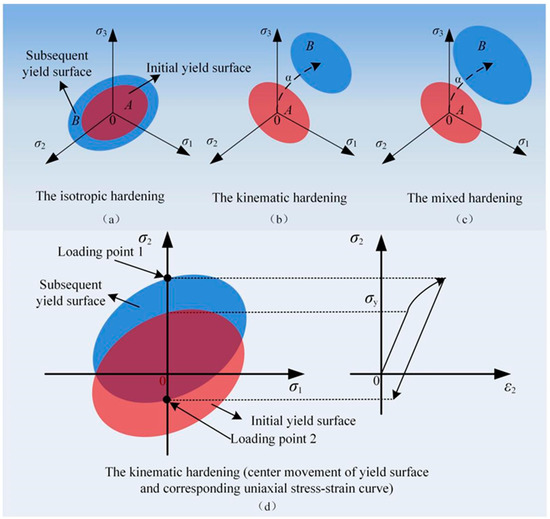
Figure 1.
Schematic diagram of yield surface variation in the classic hardening theories: (a) isotropic hardening model; (b) kinematic hardening model; (c) combined hardening model; (d) kinematic hardening (center movement of yield surface and corresponding uniaxial stress–strain curve).
The above two hardening models only describe part of the hardening behavior of materials. In plastic deformation, the yield surface of most materials undergoes both size and position changes. Therefore, when describing the hardening behavior of actual metal materials, the above two hardening models are often combined and a mixed hardening model is used, as shown in Figure 1c. Han [10] and Li Qun et al. [11] established a mixed hardening model based on the Voce isotropic hardening model and the A–F kinematic hardening model, introduced the hardening model into an equivalent drawbead resistance model, proposed an equivalent drawbead model that considered the Bauschinger effect, and verified the accuracy of the model via experiments. With the development of ABAQUS software (version 6.14, Dassault Systemes Simulia Corp., Providence, RI, USA) for finite element analysis, some parameters related to the material properties required by the kinematic hardening model and the mixed hardening model can be directly input into the software without sophisticated secondary development.
ABAQUS (version 6.14, Dassault Systemes Simulia Corp., Providence, RI, USA) provides linear and nonlinear kinematic hardening models to simulate the cyclic loading of metals. The linear kinematic model has a constant hardening modulus, which is suitable for analyzing hardening behavior with an approximately constant hardening rate. The nonlinear kinematic hardening model defines the kinematic hardening part as an incremental combination of a pure motion term (the linear Ziegler hardening rule) and a relaxation term (the recall term), so that nonlinearity is introduced to the kinematic hardening part. At the same time, in ABAQUS/Explicit, the yield stress ratio Rij of the input plate can be used with the Hill48 yield surface [12]. ABAQUS (version 6.14, Dassault Systemes Simulia Corp., Providence, RI, USA) provides three methods—assigning parameter input, assigning semi-cyclic tension-compression experiment data, and assigning sheet cyclic tension-compression experiment data to define the kinematic hardening part. The kinematic hardening material characteristic parameters obtained from the cyclic stress–strain curve of the sheet can most accurately reflect the hardening behavior of the plate under cyclic loading. The cyclic sheet tension–compression test is required to obtain the cyclic sheet tensile–compression stress–strain curve.
The buckling tendency of a thin sheet under compression is very large, and it is difficult to obtain a large compression strain. In order to obtain the tensile and compressive properties of a thin sheet under large strain, scholars have proposed various methods to suppress the buckling of the thin plate in the compression process. Boger et al. [13] used a solid plate to clamp the two sides of the thin sheet sample and applied normal pressure via a hydraulic clamping system to constrain the buckling of the thin sheet during compression. However, the thickness of the thin plate changes during the tensile–compression process, and there will inevitably be a gap between the chuck of the tensile machine and the anti-buckling fixture, resulting in excessive test error. Kuwabara et al. [14] designed a device with two pairs of comb teeth to reduce areas that are not clamped. However, the comb-tooth area is prone to bending, and the comb-tooth device is expensive. Yoshida [15] designed a special device to combine multiple samples for the tensile–compression test to overcome the defect of instability of a single sample. It measured the strain in the test process, but could not avoid the compression instability under strain. On the basis of a wedge-shaped unit designed by Cheng et al. [16], Cao et al. [17] designed an anti-buckling wedge fixture using transparent materials, which could be used to measure the whole optical strain in the deformation region of the sample by an optical strain-measurement method. Although this method can obtain tensile–compression strain under a large strain, the sample is prone to lateral instability. For the compression tests, Kurukuri [18] and Abedini et al. [19] prepared bonded sheet laminates to overcome any buckling during the tests. Due to the action of the glue between the plates, the test results had a large error, and the preparation of the sample was very complicated. In summary, in order to make the cyclic tensile–compression test of a thin sheet perform smoothly, the following three problems must be solved:
- designing a set of a reasonable thin-plate in-plane normal constraint device of thin sheets that can not only prevent the instability of the sample, but also minimize the increase in the axial compressive capacity caused by the friction force of the normal constraint;
- determining the best sample geometry that can minimize the effect of in-plane buckling and improve the accuracy of stress measurement;
- selecting a high-precision optical strain-measuring instrument in order to accurately measure the deformation of the thin sheet sample gauge.
Based on the above research, this paper aimed to establish an A–F nonlinear kinematic hardening constitutive model according to the Hill48 anisotropic yield criterion. Based on the Hill48 anisotropic yield criterion, the Voce isotropic hardening model, and the A–F nonlinear kinematic hardening model, a constitutive model inclusive of anisotropy and mixed hardening was established. A set of sheet tension–compression buckling-restrained fixtures was designed, and the shape parameters that affect stress-measurement error and inhibit in-plane buckling were determined. The optimal shape of the sample used in the in-plane compression test was determined to accurately obtain the material properties-related parameters of the kinematic hardening model and the mixed hardening model. ABAQUS (version 6.14, Dassault Systemes Simulia Corp., Providence, RI, USA) finite element software was used to analyze the applicability of the constitutive model for the cyclic tensile–compression problem of the sheets and the problem of the plate after bending, unloading, and reverse bending. The accuracy and reliability of the constitutive model were verified by experiments. This provides a reliable research method for studying the deformation behavior of sheet metal under complex loading conditions with cyclic loading characteristics.
2. Description of the Constitutive Model
2.1. Establishment and Parameter Determination of the Nonlinear Kinematic Hardening Constitutive Model
Most of the sheets used in stamping had anisotropy and a high material hardening rate, so the Mises yield criterion and the isotropic hardening model could not truly reflect the plastic behavior of the sheets during deformation. The Hill48 yield criterion considers the anisotropic characteristics of the material and considers that the contribution of stress in each direction of the sheet to the plastic yield is different, which information can be used for the plastic description of the sheet-forming process.
Assuming that the thickness anisotropy index r is constant during the plastic deformation process, if the sheet metal conforms to the flow rule of the total strain theory, then the r value can be obtained by measuring the strains in the width direction (εw) and thickness direction (εt) using a single tensile test. Specifically, the r value is expressed as follows:
The expressions for the ratio of six anisotropic yield stresses [12]—R11, R22, R33, R12, R13 and R23—can be derived by combining the Hill48 anisotropic yield conditions.
For the anisotropic behavior and the Bauschinger effect exhibited by the material during plastic deformation, the kinematic hardening model provides a simple explanation that the yield surface of the material only moves as a rigid body and does not rotate in the stress space during deformation, and the back stress represents the center of the plastic yield surface in the stress space.
The yield surface function of kinematic hardening materials is generally expressed as follows:
where is the initial yield stress and is the back stress.
The back stress represents the movement of the center of the yield surface in the stress space, which plays a crucial role in the kinematic hardening model and in yield surface evolution. Its value is related to the material hardening characteristics and deformation history. As shown in Figure 1d, the material is subjected to unidirectional elastic–plastic loading along the direction of , and the stress increases from to . During the loading process, when the deformation state of the material changes from elastic deformation to plastic deformation, the center of the yield surface begins to move. When the stress in the direction is loaded to loading point 1, unloading and reverse loading are implemented to deform the material and the material stress reaches the loading point 2 to produce reverse plastic yield. It is clear from Figure 1d that the yield stress of the material under reverse loading is smaller than the initial yield stress .
The A–F nonlinear kinematic hardening model has been extensively utilized to study the cyclic plastic behavior of materials. This model contains a linear hardening term and a dynamic restoration term. The evolution equation can be expressed as follows:
where and are material parameters; is the back stress component; is the increment in the plastic strain; is the equivalent plastic strain increment [11]; and .
When the material is subjected to uniaxial tensile loading, . Therefore, it can be determined that
The above equation can be simplified as follows:
Integrating the above first-order differential equation, we obtain
where is the initial value of the back stress and is the initial value of the plastic strain.
The initial conditions are . Using these initial values, the back stress equation can be obtained as follows:
According to the above equation, the parameters and can be determined by the nonlinear fitting of the experimentally acquired plastic strain data and the real stress obtained from the uniaxial tensile test of the sheet sample. The six anisotropic parameters (R11, R22, R33, R12, R13, and R23) and the kinematic hardening parameters ( and ) were input into the ABAQUS (version 6.14, Dassault Systemes Simulia Corp., Providence, RI, USA) material model library to obtain the material characteristic parameters related to the follow-up hardening constitutive model, based on the Hill48 yield criterion.
2.2. Establishment of the Mixed Hardening Constitutive Model
According to the Hill48 anisotropic yield criterion, combined with the Voce isotropic hardening model and the A–F nonlinear kinematic hardening model, a constitutive model that considers anisotropy and mixed hardening was established. The isotropic hardening part adopted the Voce nonlinear isotropic hardening criterion, and the equation is as follows:
where is the plastic strain, Q and b are the parameters of the isotropic hardening materials, and σ0 is the initial yield stress.
Under the uniaxial stress state, combined with the Equation (9), the material flow stress can be expressed as follows:
In order to determine the nonlinear relationship between flow stress σ and plastic strain , it is necessary to determine the four material characteristic parameters Q, b, C, and . These material characteristic parameters can be obtained by the cyclic tensile–compression stress–strain curve obtained by the sheet cyclic tensile–compression test.
2.3. Material and Experimental Procedure
The 2A11 aluminum alloy plate with a thickness of 0.6 mm was selected as the research object. 2A11 aluminum alloy is a hard aluminum alloy that is widely used in the aerospace industry, the transportation industry, and other fields. The sheet sample was cut with a line cutting machine, according to the China National Standard “Tensile testing method for metal materials at room temperature” (GB/T 228-2002). The uniaxial tensile test of the original sheet was conducted on the InspektTable-100 material universal testing machine (Huibo, Germany). The standard size of the sheet sample used in the unidirectional tensile test was 50 mm. Three groups of unidirectional tensile samples were cut along the directions of 0°, 45°, and 90° with respect to the rolling direction. The strain rate during the tensile test was 0.0013/s. To obtain the anisotropy coefficient, the axial strain, and the transverse strain during the deformation process of the sample were recorded by an online strain-measurement system based on digital image correlation (DIC). The testing machine and the DIC online strain-measurement system are shown in Figure 2a, and the size of the uniaxial tensile sample is shown in Figure 2b.
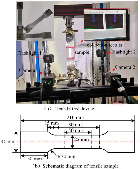
Figure 2.
Uniaxial tensile test diagram of 2A11 aluminum alloy sheet: (a) test drawing machine diagram; (b) uniaxial tensile sample.
The engineering stress–strain curve of the large sample was obtained by the uniaxial tensile test, and the real stress–strain data were obtained according to the conversion formula, as shown in Figure 3a. In the uniaxial tensile process of the sample in three directions, the strains in the width and thickness directions were measured to obtain the r value, and the results are shown in Figure 3b. According to Equation (9), the initial yield point in the real stress–strain curve of 2A11 aluminum alloy sheet was taken as the starting point of the back stress parameter fitting curve for obtaining the relevant parameters. The parameters of each material model are listed in Table 1 and Table 2.
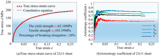
Figure 3.
(a) True stress–strain curve of 2A11 aluminum alloy sheet; (b) anisotropy coefficient of 2A11 aluminum alloy sheet.

Table 1.
Simulation of material parameters required.
Table 2.
Ratio of anisotropic yield stress of materials.
3. Cyclic Sheet Tension-Compression Test and Sample Shape Optimization
3.1. Shape Optimization of Cyclic Sheet Tension-Compression Sample
The cyclic tensile–compression test of aluminum bars is relatively easy to perform and there are corresponding standards to follow [20,21]. However, an aluminum alloy sheet is prone to instability during compression, and the optimum sample shape to minimize the stress-measurement error and suppress the in-plane buckling of the sample has not yet been defined [22]. Therefore, this study used the finite element method (FEM) to identify the shape parameters that had an effect on the stress-measurement error and the shape parameters that had an effect on the suppression of in-plane buckling to determine the optimum shape of the sample for use in the cyclic tension-compression tests.
Figure 4 represents the shape parameters of the sheet tensile–compression sample evaluated in this study. The width and length of the parallel section are W and L, respectively; the radius of the fillet of the transition section between the parallel section and the clamping end is R; the width of the clamping end is B and the length of the clamping end was determined by the clamping head size of the test machine and was set at 30 mm.
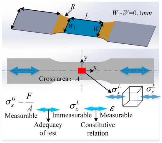
Figure 4.
Geometrical parameters of the sample for in-plane compression test and schematic illustration of the difference between mean stress and local stress .
When a sheet tensile–compression sample was subjected to in-plane compression, the deformation within the parallel section was not uniform due to the transition section constraining the deformation near the ends of the parallel section, resulting in inconsistent compressive stresses. Therefore, the sample shape had to be optimized to improve the accuracy of the stress measurement. In addition, in order to retard the onset of in-plane buckling and to allow greater compression to be applied, shape parameters that helped to suppress in-plane buckling had to be defined to optimize the cyclic drawing of the sheet samples.
In the cyclic sheet tensile–compression test, the average stress can be found from the compression force F and the area of the central section of the sample derived from the constant volume criterion. However, the local stress at the center of the sample in the experiment could not be obtained in the sample and could be extracted in the post-processing results of the FEM. The smaller the difference between the absolute value of the local stress and the mean stress in the central part of the sample, the higher the accuracy of the stress measurement. Therefore, the FEM was used to analytically determine the sample shape that minimizes the difference between the local stress and the mean stress .
The relative deviation of from is given by the following equation:
The smaller the sample shape, the greater the accuracy of the stress measurement.
The deformation was not uniform in the parallel part of the sample, due to cyclic tension–compression. To clarify the sample shape parameters that inhibit surface buckling using the FEM, the width difference W-W1 = 0.05 mm between the two ends of the parallel section was set as the initial unevenness to perform the buckling analysis. Under compression, the parallel section of the sample will produce shear stress . The ratio of shear stress in the central part of the sample to local stress was used to determine the buckling of the sample. The determination formula of in-plane buckling is as follows:
The smaller the , the less the possibility of buckling during compression.
3.2. FEM Model for Sample Shape Optimization
To obtain the optimum sample shape for the cyclic sheet tensile–compression test, a finite element model for the cyclic sheet tensile–compression test was established, as shown in Figure 5a. The aspect ratio of the deformation zone to the width of the clamping end B and the corner radius R of the corner transition zone had a great influence on the accuracy of the stress measurement and the compression limit, so a variety of dimensional parameters were set for the FEM analysis, as shown in Figure 5b. The clamping plates on both sides of the sample deformation zone were always clamped with a clamping force of 940 N. The clamping plates on both sides of the clamping end were bound together with the clamping end of the sample. The friction coefficient between the cyclic tension–compression sample and the clamping plates was set to 0.084. The strain rate during the cyclic tension-compression test was 0.0013/s. In the finite element model for the cyclic sheet tensile–compression test, the cyclic sheet tensile–compression sample was set up as a deformed body and all the remaining components were defined as rigid bodies. The sample was set up with five integration points in the thickness direction by applying a four-node curved thin-shell or thick-shell reduction integral, an S4R cell with finite film strain, and an hourglass control. The element size of the sample was set to 0.5 mm to ensure that no distortion occurred in the process of compression, so as to obtain accurate stress calculation results.
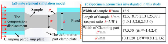
Figure 5.
(a) Finite element simulation model; (b) sample geometries investigated in this study.
3.3. Sample Shape Optimization Simulation Results
3.3.1. Effect of Sample Deformation Zone Aspect Ratio and Clamping End Width B
During the compression of the cyclic sheet tensile–compression sample, B/W = 1.4, R/W = 1.2; B/W = 2.4, R/W = 1.2 were set to investigate the effect of the aspect ratio of the deformation zone of the sample and the width B of the clamping end. From the simulation results, as shown in Figure 6a,b, when the width B of the sample clamping end and the radius R of the fillet area were certain, the stress-measurement accuracy gradually increased with the increase in the sample deformation zone aspect ratio . The stress-measurement accuracy decreased due to the increase in the length of the sample deformation zone and the influence of the corner area on the measurement accuracy became smaller when the width of the clamping end B was too large. Buckling was more likely to occur when the sample deformation zone was too long, as shown in Figure 6c,d. The wider the sample clamping end, the more serious the deformation of the rounded area as the transition area, which exerted more influence on measurement accuracy. From the simulation results and the above analysis, it can be seen that the longer the deformation zone of the sample, the higher the accuracy of the stress measurement, but buckling was also more likely to occur; therefore, the best aspect ratio of the deformation zone of the sample was moderately chosen as λ = 2. The deformation of the fillet area of the sample directly affects the accuracy of the stress measurement, so it was necessary to investigate the influence of the shape and size of the fillet area on the accuracy of the stress measurement.
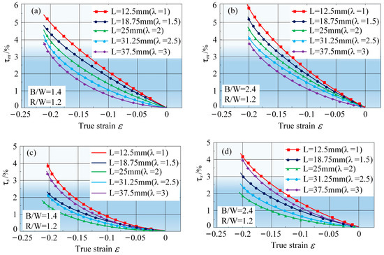
Figure 6.
Effect of aspect ratio λ on the variation of and with true strain: (a) B/W = 1.4; (b) R/W = 1.2; (c) B/W = 2.4; (d) R/W = 1.2.
During the compression of the cyclic sheet tensile–compression sample, B/W = 1.4, R/W = 1.2; B/W = 2.4, R/W = 1.2 were set to investigate the effect of the aspect ratio of the deformation zone of the sample and the width B of the clamping end. From the simulation results, as shown in Figure 6a,b, when the width B of the sample clamping end and the radius R of the fillet area were certain, the stress-measurement accuracy gradually increased with the increase of the sample deformation zone aspect ratio .
3.3.2. Effect of Fillet Radius R in the Fillet Area of the Sample
Applying B/W = 1.4, λ = 2, different sizes of fillet radius R were set to analyse the effect on stress-measurement accuracy and buckling. The simulation results are shown in Figure 7. An increase in the fillet radius improved the accuracy of stress prediction and it was less likely that buckling occurred. The reason for this was that the large fillet radius area weakened the restraint on both ends of the parallel section, so the parallel section deformed more uniformly and was less likely to buckle.
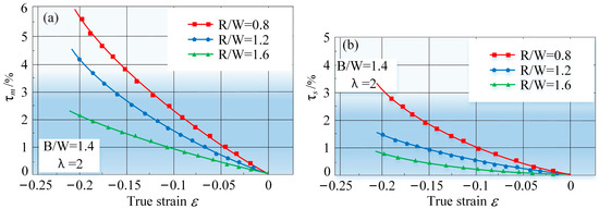
Figure 7.
Effect of fillet radius R on (a) and (b) .
3.3.3. Influence of n-Values of the Sample
With sheets of different materials, n-values (the strain hardening exponent in Swift’s equation) vary widely, and it is known from studies related to buckling formation that the larger the n-value of the sheet, the less likely it is to buckle [23]. The uniaixal tensile curve of 2A11 aluminum alloy sheet was fitted and its n value was obtained as 0.3468. The n-values of 0.2, 0.3468 and 0.5 were set, and the parallel section aspect ratio λ = 2 and B/W = 1.4 were used for FEM analysis. The results are shown in the Figure 8. With the increase in n-value, the stress-measurement accuracy was higher and the tensile samples were less likely to buckle during the compression process. In summary, the sheets with large n-values had a higher stress-measurement accuracy in sheet drawing and in the cyclic sheet tensile–compression test, due to stable deformation and the sample was less prone to buckling; the plates with large n-values had better forming performance in stamping and forming with cyclic loading characteristics.
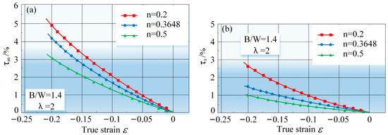
Figure 8.
(a) Effect of n-values on ; (b) Effect of n-values on .
Based on the above analysis of the FEM results for the optimization of the cyclic sheet tensile–compression sample shape, it can be seen that the sample shape with a moderate aspect ratio of parallel sections and larger radius of fillet was selected for higher accuracy of stress measurement and less susceptibility to buckling. The final determination of the shape and size of the cyclic sheet tensile–compression sample is shown in Figure 9b.
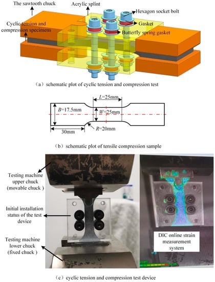
Figure 9.
Cyclic tensile–compression test: (a) schematic diagram of cyclic tension and compression test; (b) schematic drawing of used tensile–compression specimen; (c) cyclic tension and compression test device.
3.4. The Cyclic Sheet Tensile–Compression Test
To obtain the cyclic tensile–compression stress–strain curves of the studied sheets, an anti-buckling fixture was designed, as shown in Figure 9a. The cyclic tensile–compression test of the studied sheets used the specimen geometry of Figure 9b. The anti-buckling fixture was made of transparent acrylic sheets on both sides as raw material, and optical strain-measurement equipment was used to accurately measure the strain change of the sample. The transparent acrylic sheet did not affect the DIC camera’s shooting, as shown in Figure 9c. The sheet had a change in thickness during the tensile–compression process, so the disc spring placed between the bolt and the clamping plate ensured that the clamping plate was always clamping elastically during the clamping process.
The relative sliding between the tensile–compression sample and the clamping plate generated friction, and the direction of the friction force was opposite to the direction of the movement of the tester chuck, making the load measured by the tester large. Assuming that the friction force was uniformly distributed on the contact surface, the Coulomb friction formula was applied to calculate the magnitude of the friction force during the test, and the friction force was removed from the measured test data to eliminate the error caused by friction on the load measurement. In order to determine the friction coefficient between the sheet and the clamping plate, the friction coefficient between the 2A11 aluminum alloy sheet and the acrylic plate was tested using a friction and wear tester produced by the Center for Tribology (CETR) in the United States The friction coefficient, using transparent silicone oil as a lubricant, was 0.084. The anti-buckling fixture was used to perform cyclic tensile–compression tests on sheet metal on the InspektTable-100 material universal testing machine, and the strain changes during sample deformation were recorded by the DIC online strain-measurement system.
The disc spring gasket was of type A (GB/T1972-2005), with dimensions of outer diameter φ10 mm, inner diameter φ5.2 mm, thickness 0.5 mm, initial height 0.75 mm, and compressible amount 0.25 mm. The disc springs buckled in two groups of the same specification, each group made up of three stacked disc springs, and the combined buckling disc spring group was compressed by 0.75 mm, as shown in Figure 10a, while the stiffness curve of the single group of disc springs was measured by the InspektTable-100 material universal testing machine (Huibo, Germany). In the cyclic sheet tensil–compression test, the pre-compression of the disc spring group was 0.3 mm, and the total clamping force of the four groups of disc springs varied with the thickness of the sample, as shown in Figure 10b. The cyclic stress–strain curve for the selected specimen of Figure 9b, after eliminating the effect of fixture friction, is shown in Figure 10c. Similar data were obtained by many cyclic tensile–compression tests, and the test results were reliable.
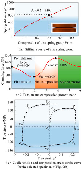
Figure 10.
(a) Stiffness curve of butterfly spring group/mm; (b) tension and compression process node; (c) cyclic tension and compression stress–strain curve for the selected specimen of Figure 9b.
3.5. Determination of the Mixed Hardening Constitutive Model Parameter
The flow stress and the equivalent plastic strain in the constitutive model were nonlinearly mapped, and there were many parameters. In order to obtain each parameter of the constitutive model accurately, the solution was based on the cyclic sheet tensile–compression stress–strain curve. The material flow stress in the uniaxial stress state in uniaxial tension for the mixed hardening constitutive model can be expressed as follows:
When the uniaxial tension reached and the plastic pre-strain was equal to during reverse loading and unloading, the flow stress was calculated as follows:
When it is reverse loading to , it is reverse loading again. At this time, the plastic strain is , and the flow stress is as follows:
Let , , , and , and through the summary Equations (12)–(14), it can be obtained that the general stress-strain equation in the process of the uniaxial cyclic tension-compression loading process is as follows:
where, A, B, C, and E are material constants that can be obtained by fitting the cyclic tensile–compression stress–strain curve derived from the cyclic sheet tensile–compression test, and D is a constant related to the direction of the pre-strain, with a plus sign for the forward direction and a minus sign for the reverse direction.
According to the cyclic tensile–compression stress–strain curves derived from the cyclic tensile–compression tests, four material characteristic parameters—Q, b, C, and —in the mixed hardening model can be obtained by fitting. The goodness of fit R2 was 0.99 and the fitting accuracy was high. Q and b are the parameters related to isotropic hardening; C and are the parameters related to kinematic hardening, as shown in Table 3.
Table 3.
Parameters obtained in the combined hardening model.
4. Reliability Analysis of the Constitutive Model
4.1. The Application of the Constitutive Model in the Cyclic Sheet Tensile–Compression Problem
The material characteristic parameters of the A–F nonlinear kinematic hardening constitutive model, based on the Hill48 anisotropic yield criterion, and the material characteristic parameters of the mixed hardening constitutive model, based on the Hill48 anisotropic yield criterion, the Voce isotropic hardening model, and A–F nonlinear kinematic hardening model, were input into the cyclic sheet tensile–compression simulation model. The simulation results of the two constitutive models were compared with the experimental results, as shown in Figure 11.
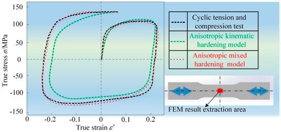
Figure 11.
Fitting and calibration of constitutive elastic–plastic material model parameters and comparison of simulation and experimental results.
In the initial tensile stage, the simulated results of the two constitutive models were in general agreement with the experimental results. When the sheet was subjected to tensile deformation unloading, and reverse compression, the simulated results deviated from the experimental results, with an average deviation of 7.4% for the simulated results of the kinematic hardening model and 2.1% for the simulated results of mixed hardening model. When the sheet was stretched again, the average deviation of the simulated results of mixed hardening model was 1.3%, while the average deviation of the simulated results of kinematic hardening model was 11.7%.
4.2. The Application of the Constitutive Model in the Continuous Bending Problem
The kinematic hardening model and the mixed hardening constitutive model were applied to the simulation of continuous bending, straightening, and reverse bending deformation. The FEM model was established for simulation analysis, as shown in Figure 12. The continuous bending model structural parameters were as follows: the transitions rounding of the upper and lower die were 7.34 mm and 8 mm, respectively; the radii of the semicircular rounding of the upper and lower die were 8.66 mm and 8 mm, respectively; the 2A11aluminum alloy sheet with a thickness of 0.6 mm was chosen as the object of study, and the sheet’s length, width, and thickness were 100 mm, 10 mm, and 0.6 mm, respectively. After the upper and lower die closed the die, a gap of 0.06 mm was retained. A 4-node reduced integration S4R unit was used to divide the sheet, and five integration points were set in the sheet thickness direction. In order to ensure the smooth progress of the continuous bending test, no fracture occurred in the sample, Coulomb friction was used between the contact surface of the upper and lower die and the sheet, and the friction factor was set to 0.096. The front end of the sheet was bound to the pulling plate and the displacement constraint was used.
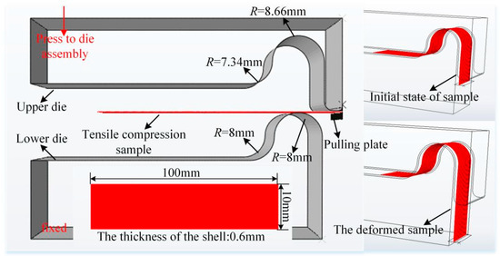
Figure 12.
Finite element simulation model.
The material characteristic parameters of the A–F nonlinear kinematic hardening constitutive model, based on the Hill48 anisotropic yield criterion, and the material characteristic parameters of the mixed hardening constitutive model, based on the Hill48 anisotropic yield criterion, the Voce isotropic hardening model, and the A–F nonlinear kinematic hardening model, were input into the sheet continuous-bending model and compared with the sheet continuous-bending test for analysis.
The continuous-bending test die of the sheet is shown in Figure 13. Figure 13a,b show the upper and lower die of the continuous bending test die, respectively, and the size is the same as the size of the die in the simulation model. The upper and lower dies were fixed by bolts, and the upper chuck of the InspektTable-100 material universal testing machine clamped the clamping end of the upper die, and the lower chuck of the universal testing machine clamped the lower end of the continuous bending sample, as shown in Figure 13c. In the continuous-bending test, the specimen was easy to break because of the large bending deformation. In order to ensure the smooth progress of continuous-bending test without fracturing the sample, an oil-based molybdenum disulfide lubrication was applied between the continuous-bending sample and the mold, and the friction coefficient was 0.096. During the test, the upper chuck was fixed and the lower chuck was moved down at a constant speed of 50 mm/min. The state of the continuously bent sample after the die assembly and after experiencing continuous bending is shown in Figure 13d.
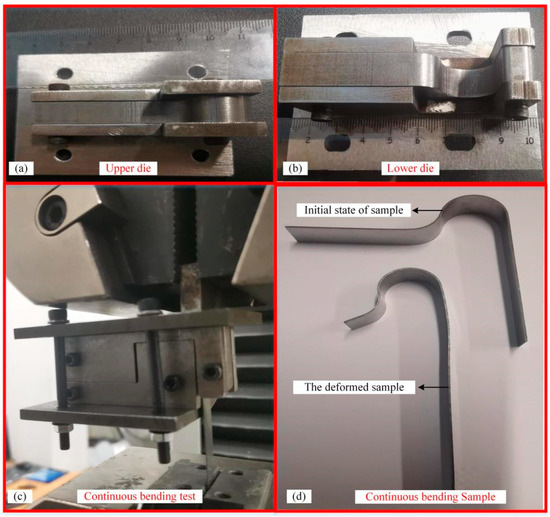
Figure 13.
(a) Upper die; (b) Lower die; (c) Continuous bending test die; (d) Continuous bending Sample.
Figure 14 shows the results of the comparison between the lower chuck tension during the continuous-bending test and the pulling plate tension in the simulation results. The computational error of the mixed hardening model is smaller than that of the kinematic hardening model and is closer to the test value. The wall thickness distribution of the sample after continuous bending was measured with a micrometer and compared with the simulation results of the two constitutive models in the same state. The wall-thickness distribution of the samples in the simulation results of the kinematic hardening model and the mixed hardening model was consistent with the trend of the experimental results, and the simulation results of the mixed hardening model were closer to the experimental results, with little deviation. It was demonstrated that the material characteristic parameters of the mixed hardening constitutive model, based on the Hill48 anisotropic yield criterion, the Voce isotropic hardening model, and the A–F nonlinear kinematic hardening model, can be used to study the continuous-bending deformation behavior of the sheet under a complex loading condition, and its calculation results are reliable.
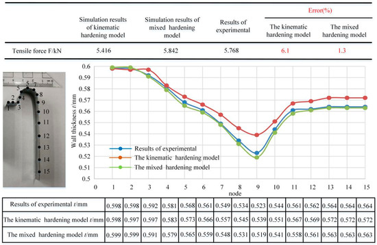
Figure 14.
Comparison between FEM results and experimental results.
4.3. Application of Constitutive Model in the Springback Problem
A three-point bending FEM model was created, as shown in Figure 15, to test the correctness of the two constitutive models used to simulate the springback issue. The three-point bending test model’s indenter diameter was 20 mm, the support point diameter was 30 mm, the distance between the two support points was 100 mm, and the three-point bending sample’s length, width, and thickness were 120 mm, 20 mm, and 0.6 mm, respectively. The sheet material was divided into five integration points in the direction of the sheet thickness using a 4-node reduced integration S4R cell. Coulomb friction was used between the contact surfaces, and the friction factor was set to 0.1. Two support points were fixed, and the indenter was constrained by displacement. The material characteristic parameters of the A–F nonlinear kinematic hardening constitutive model, based on the Hill48 anisotropic yield criterion, and the material characteristic parameters of the mixed hardening constitutive model, based on the Hill48 anisotropic yield criterion, the Voce isotropic hardening model, and the A–F nonlinear kinematic hardening model, were input into the sheet three-point bending model and compared with the three-point bending test for analysis.
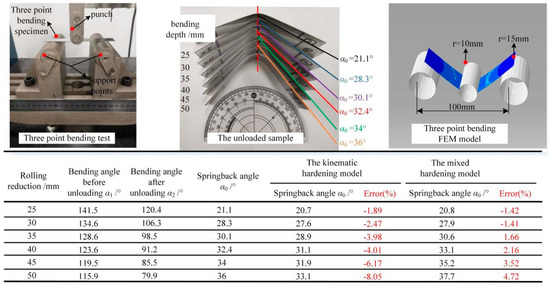
Figure 15.
Comparison of the FEM results and the experimental results.
In sheet metal forming, the prediction of springback is important to show the desired final geometrical quality of the parts. Figure 15 presents the final result after springback was obtained from the kinematic hardening model, the mixed hardening model, and the experimental results. The results of the mixed hardening model matched the experimental data with superior accuracy than the results of the kinematic model, according on comparisons of the final shapes after the anticipated springback.. This proved that the mixed hardening model implemented in ABAQUS (version 6.14, Dassault Systemes Simulia Corp., Providence, RI, USA) can be applied for an accurate prediction of springback in complex industrial sheet metal forming operations.
5. Conclusions
(1) The FEM analysis of the in-plane compression sample quantitatively specified the shape parameters that minimize the measurement error of compressive stress and help to suppress in-plane buckling. A transparent anti-buckling fixture was designed to accurately measure the strain variation of the cyclic tensile–compression sample using optical strain-measurement equipment.
(2) An anisotropic mixed hardening constitutive model based on the Hill48 anisotropic yield criterion, the Voce isotropic hardening model, and the A–F nonlinear kinematic hardening model was established. The cyclic deformation stress–strain curves of 2A11 aluminum alloy sheet were obtained by cyclic sheet tensile–compression tests, and the material characteristic parameters in the mixed hardening model were accurately determined. The obtained material characteristic parameters were directly input into the Abaqus simulation software, eliminating the need for tedious secondary development.
(3) The reliability and accuracy of the established constitutive model for anisotropic mixed hardening materials were verified through finite element simulations and tests of the aluminum alloy sheet cyclic tension-compression problem, the springback problem, and the sheet in bending, unloading, and reverse bending problems. It provided a reliable research tool for predicting the deformation behavior of the sheet under complex loading conditions with cyclic loading characteristics.
Author Contributions
Conceptualization, G.C.; methodology, G.C., Q.Z. and C.W.; software, G.C. and H.S.; validation, C.Z., Q.Z. and D.C.; formal analysis, C.Z.; investigation, C.Z., H.S., Z.L., C.W. and D.C.; resources, G.S.; data curation, G.S.; writing—original draft preparation, H.S.; writing—review and editing, G.C.; visualization, Z.L.; supervision, G.C.; project administration, G.C.; funding acquisition, G.C. All authors have read and agreed to the published version of the manuscript.
Funding
This research received no external funding.
Institutional Review Board Statement
Not applicable.
Informed Consent Statement
Not applicable.
Data Availability Statement
All data were obtained by the author through experiment.
Conflicts of Interest
The authors declare no conflict of interest.
References
- Hu, H.; Hong, X.; Tian, Y.; Zhang, D. Az31 magnesium alloy tube manufactured by composite forming technology including extruded-shear and bending based on finite element numerical simulation and experiments. Int. J. Adv. Manuf. Tech. 2021, 115, 2395–2402. [Google Scholar] [CrossRef]
- He, B.; Huang, S.; He, X. Numerical simulation of gear surface hardening using the finite element method. Int. J. Adv. Manuf. Tech. 2014, 74, 665–672. [Google Scholar] [CrossRef]
- Xin, C. Establishment and Application of Elastic-Plastic Constitutive Model for Cyclic Loading. Doctoral Dissertation, Yanshan University, Yanshan, China.
- Li, Q.; Xin, C.; Jin, M.; Zhang, Q. Establishment and application of an anisotropic nonlinear kinematic hardening constitutive model. Chin. J. Mech. Eng. 2006, 42, 6. [Google Scholar] [CrossRef]
- Xiao, Y.Z.; Chen, J. A review of research in macroscopic hardening models in numerical simulation of sheet metal forming. Int. J. Plast. 2009, 16, 8. [Google Scholar]
- Ziegler, H. A modification of prager’s hardening rule. Q. Appl. Math. 1959, 17, 55–65. [Google Scholar] [CrossRef]
- Armstrong, P.J.; Frederick, C.O. A mathematical representation of the multiaxial bauschinger effect. Mater. High Temp. 2007, 24, 1–26. [Google Scholar]
- Yu, H.Y. Comparative study on strain hardening models of thin metal sheet. Forg. Stamp. Technol. 2012, 37, 6. [Google Scholar]
- Yu, H.Y.; Wang, Y. A combined hardening model based on chaboche theory and its application in the springback simulation. Chin. J. Mech. Eng. 2015, 51, 8. [Google Scholar] [CrossRef]
- Han, C.; Dong, X.H. An equivalent drawbead model considering Bauschinger effect. Forg. Stamp. Technol. 2017, 42, 7. [Google Scholar]
- Li, Q.; Jin, M.; Zou, Z.Y.; Guo, J.; Yang, C. Parameter determination and application research of mixed hardening model based on cyclic tension-compression test. Chin. J. Mech. Eng. 2020, 2, 6. [Google Scholar] [CrossRef]
- Chen, G.; Zhao, C.C.; Yang, Z.Y.; Dong, G.J.; Cao, M.Y. Effects of Q235 Coated Tubes on Bulging Behavior of AA5052 Aluminum Alloy Base Tube with Granular Medium. Chin. J. Mech. Eng. 2021, 32, 10. [Google Scholar]
- Boger, R.K.; Wagoner, R.H.; Barlat, F.; Lee, M.G.; Chung, K. Continuous, large strain, tension/compression testing of sheet material. Int. J. Plast. 2005, 21, 2319–2343. [Google Scholar] [CrossRef]
- Kuwabara, T.; Kumano, Y.; Ziegelheim, J.; Kurosaki, I. Tension-compression asymmetry of phosphor bronze for electronic parts and its effect on bending behavior. Int. J. Plast. 2005, 25, 1759–1776. [Google Scholar] [CrossRef]
- Yoshida, F.; Uemori, T. Cyclic Plasticity Model for Accurate Simulation of Springback of Sheet Metals; Springer Vieweg: Berlin/Heidelberg, Germany, 2015; pp. 65–66. [Google Scholar]
- Jian, C.; Lee, W.; Hang, S.C.; Seniw, M.; Chung, K. Experimental and numerical investigation of combined isotropic-kinematic hardening behavior of sheet metals. Int. J. Plast. 2009, 25, 942–972. [Google Scholar]
- Hang, S.C.; Lee, W.; Jian, C.; Seniw, M.; Chung, K. Experimental and Numerical Investigation of Kinematic Hardening Behavior in Sheet Metals. In Proceedings of the 10th Esaform Conference on Material Forming, Zaragoza, Spain, 18–20 April 2007; Volume 907, pp. 337–342. [Google Scholar]
- Kurukuri, S.; Worswick, M.J.; Ghaffari Tari, D.; Mishra, R.K.; Carter, J.T. Rate sensitivity and tension-compression asymmetry in AZ31B magnesium alloy sheet. Philos. Trans. 2014, 372, 20130216. [Google Scholar] [CrossRef] [PubMed]
- Abedini, A.; Butcher, C.; Nemcko, M.J.; Kurukuri, S.; Worswick, M.J. Constitutive characterization of a rare-earth magnesium alloy sheet (ZEK100-O) in shear loading: Studies of anisotropy and rate sensitivity. Int. J. Mech. Sci. 2017, 128, 54–69. [Google Scholar] [CrossRef]
- Ma, M.T. A review of the Bauschinger effect in metals and alloys. Mater. Mech. Eng. 1986, 10, 15–21. [Google Scholar]
- Wang, Y.F.; Li, C.; Ling, X.Y.; Shen, B.L.; Gao, S.J.; Ying, S.H. An overview on the Bauschinger effect in metallic materials. China Nucl. Sci. Technol. Rep. 2002, 1, 14. [Google Scholar]
- Noma, N.; Kuwabara, T. Numerical investigation of specimen geometry for in-plane compression tests and its experimental validation. J. Jpn. Soc. Technol. Plast. 2012, 53, 574–579. [Google Scholar] [CrossRef]
- Dong, X.H. Principles of Metal Forming; China Machine Press: Beijing, China, 2011; pp. 154–196. [Google Scholar]


Disclaimer/Publisher’s Note: The statements, opinions and data contained in all publications are solely those of the individual author(s) and contributor(s) and not of MDPI and/or the editor(s). MDPI and/or the editor(s) disclaim responsibility for any injury to people or property resulting from any ideas, methods, instructions or products referred to in the content. |
© 2023 by the authors. Licensee MDPI, Basel, Switzerland. This article is an open access article distributed under the terms and conditions of the Creative Commons Attribution (CC BY) license (https://creativecommons.org/licenses/by/4.0/).