Abstract
The Johnson–Cook model is widely used because of its ability to meet the simulation material requirements in various situations. However, under different working conditions, the accuracy of the model may have errors. In this work, based on Abaqus (Abaqus R2022 Education Edition, Dassault Systèmes, Paris, France) simulation software, Johnson–Cook (JC) constitutive model parameters and compression parameters were selected to simulate the improvement of surface roughness during the ball milling of a 7075-T651 aluminum alloy. In the numerical simulation of ball polishing, the changes in the residual stress field when the Johnson–Cook parameters change are analyzed. By comparing the numerically simulated residual stress fields under the JC parameters calculated at different strain rates, a set of parameters that agrees with the experimental values is selected. The results show that the residual stresses are in line with the experimental values when the strain rate is 10−4s −1. The changes in roughness corresponding to the selected parameters are analyzed. The results indicate that the simulated trend of roughness variation is consistent with the experimental values, and the optimal surface roughness value under a static pressure of 300 N is obtained.
1. Introduction
The 7075 aluminum alloy is widely used in the aerospace field because of its low density (2.81 g/cm3) and high yield strength, which exceeds 500 MPa []. In the aerospace field, due to its harsh service environment, higher requirements are put forward for the surface properties of materials. Ball burnishing is a traditional processing method that can improve the surface hardness and fatigue strength of the material and reduce its surface roughness. For example, F. Klocke et al. [] reduced the average peak-to-valley height Rz by 30% to 50% by applying ball burnishing to the surface of the turned material. P. Zhang et al. [] discovered that by applying ball burnishing to an Mg-12Gd-3Y magnesium alloy, the fatigue life of the as-rolled alloy and aging heat-treated alloy was increased by about 50% and 36%, respectively. Through TA2 alloy ball burnishing research, X. L. Yuan et al. [] concluded that, compared with the original machined surface, the hardness was increased by 28% and the surface roughness was reduced by 63%. In addition, compared with grinding and polishing technology, ball burnishing could improve hardness and fatigue strength in a short time, saving at least 1 h [,].
Ball burnishing also offers significant advantages over some other traditional processes. For example, M. Hilpert et al. [] employed mechanical burnishing, shot peening, and ball burnishing to treat the surface of the high-strength magnesium alloy AZ80. The results showed that the surface after ball burnishing not only obtained good fatigue performance but also showed superior corrosion fatigue properties in a 3.5% NaCl solution. In a study of an AZ80 magnesium alloy using shot peening and ball burnishing, P. Zhang et al. [] also pointed out that, under a static pressure of 200 N, the fatigue strength of the alloy after the ball burnishing treatment increased by 110%, and that rolling was more beneficial for improving fatigue life than shot peening.
Scholars have carried out research on the relationship between ball burnishing processing parameters and the processing effect. Ball burnishing parameters include spindle speed, static pressure, the number of passes, and feed rate. The parameters have a significant impact on the properties of materials, such as hardness and fatigue strength. M. H. El-Axir et al. [] researched the effects of spindle speed and the number of passes on the microhardness of an St-37 alloy. They found that the microhardness of the material increased by 68% at a pass count of three and a spindle speed of 450 r/min. M. El-Khabeery et al. [] conducted ball burnishing research on a 6061-T6 aluminum alloy and found that low feed speed and high static pressure were conducive to decreasing the material’s surface roughness. In the study of V. Barahate et al. [], an AA6061-T6 alloy was ball burnished using the Taguchi method to study the impact of processing parameters on the surface finish. The results showed that, with a degree of influence of 54.51%, the feed rate had the highest impact on the material’s surface roughness.
In terms of ball burnishing numerical simulation, studies were first based on a 2D model, and then 3D ball burnishing models were presented. For example, Y. C. Yen et al. [] established 2D and 3D ball burnishing models to research surface deformation and residual stress, but the size of the 3D model was too small, and the experimental results were not consistent enough. The findings demonstrated that the 3D model exhibits a more realistic surface deformation while the 2D model has a greater ability to forecast changes in residual stress. P. Sartkulvanich et al. [] established 2D ball burnishing models and investigated how the feed rate and static pressure affected roughness and residual stress using the 2D model. The results showed that the models predicted the average roughness well. The error between the experimental results and the tangential residual stress results was 4%. P. Balland et al. [] provided ideas for modeling 3D models, including establishing local 3D models of actual working conditions, replacing the whole with a small part, and introducing finite element mesh elements, which provided the feasibility of 3D modeling. D. Zhang et al. [] used the established 3D model to analyze residual stress and deformation and found that the residual stress distribution trend corresponded to the experimental results, but the measured value was about 80 MPa lower than the simulated value. G. V. Duncheva et al. [] researched the influence of static pressure, number of passes, and feed rate on residual stress through the established 3D finite element model. When the X-ray residual stress findings were compared, it was discovered that the distribution trend of the two was consistent. G. Rotella et al. [] studied the impact of the combined turning/burnishing process on the surface integrity of the Ti6Al4V alloy using the 3D rolling model created by the SFTC Deform 3D program, and successfully foresaw changes in grain size, dislocation, residual stress, and hardness. D. Borysenko et al. [] created a 3D finite element model using 3D scanning to simulate the true morphology, taking into account how the ball burnishing process was affected by the initial roughness, and the results showed that, compared with the traditional smooth surface model, the deviation between the axial force and the test was reduced from 6.17% to 1.45%, and the feed force deviation was reduced from 11.23% to 1.4%. Although the above-mentioned scholars have obtained many phased results through numerical simulation technology, the problem of numerical simulation accuracy has always been the focus of research. The effects on the precision of ball burnishing numerical simulation are manifold, and material parameters are one of the most important aspects. For transient dynamic analyses, the constitutive equation will significantly affect the accuracy of the simulation results [].
The Johnson–Cook (JC) model can satisfy simulated material needs in a variety of circumstances []. Although the model fully takes into account the link between temperature, strain, and strain rate, it does not take into account the coupling effects between different factors. Therefore, under different working conditions, there will be errors in the accuracy of the model. In this regard, scholars have conducted a lot of research. By adding a strain hardening coefficient that fluctuates with the strain and strain rate to the JC model of the 7050-T7451 aluminum alloy, J. Tan [] et al. found that the model was better able to predict the tensile flow behavior of the alloy at high strain rates. The JC model modified by Y. Zhao et al. [] incorporated the coupling effects of the deformation temperature, strain rate, strain rate softening effect, and flow strain stress, and the improved model accurately forecasted the dynamic behavior of the laser additive manufactured FeCr alloy. L. Niu et al. [] considered the thermal softening mechanism of the A356 alloy, and the modified JC model’s average absolute error was 1.46%. Y. Wang et al. [] modified the JC model with a new temperature term, and the error between the prediction data of the model and the experimental results was within 5%. Compared with all the research discussed above, the JC parameter study of ball burnishing has been rarely reported [,].
In this paper, the problem of the accuracy of the numerical simulation of rolling using JC parameters is studied, and a method to modify the JC parameters is proposed. The residual stress field of the ball burnishing simulation is analyzed using compression parameters and JC parameters. The Johnson–Cook parameters were reverse adjusted by comparing the numerical simulation residual stress field of the Johnson–Cook parameters and the compression curve parameters. The simulation results using the modified JC parameters were compared with the experimental results to verify the accuracy of the modified JC model.
2. Materials and Methods
2.1. Experimental of Ball Burnish
The experimental material was a 7075-T651 aluminum alloy bar with a diameter of 50 mm. The chemical composition of the 7075-T651 alloy is shown in Table 1.

Table 1.
Chemical composition of 7075-T651 alloy (wt.%).
The ball burnishing process of the 7075-T651 alloy is shown in Figure 1a. is a schematic diagram of the ball burnishing process, and Figure 1b. is the actual ball burnishing process, with a cemented carbide ball with a 15-mm diameter on top that can rotate freely, and a spring at the tail to provide the initial static pressure. The ball burnishing equipment was fixed on the CW6163C (Dalian machine tool, Dalian, China) lathe tool holder. The specimen was fixed between the support chucks. Different static pressures can be applied by changing the amount of compression in the spring.
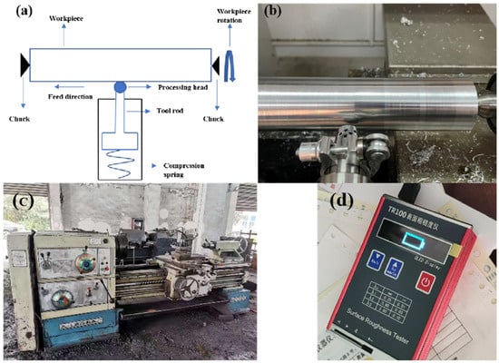
Figure 1.
Ball burnishing process of 7075-T651 aluminum alloy: (a) schematic diagram of ball burnishing processing; (b) actual ball burnishing process; (c) CW6163C lathe; (d) TR100 roughness meter.
The bar’s original surface has an oxide layer on it, and the existence of the oxide film will have a certain impact on the processing process. Therefore, the outer skin of the material shall be removed before ball burnishing. In order to obtain better test results, the research results of other scholars were consulted when selecting processing parameters [,,]. The turning parameter was a lathe speed of 240 r/min, and the feed rate was 0.2 mm/r. The ball burnishing process parameters are shown in Table 2. The spindle speed was 240 r/min, the feed rate was 0.1 mm/r, the static pressure was 150 N, 300 N, and 600 N, respectively. The average surface roughness (Ra) was extracted using the TR100 (Beijing time-top technology Co., Ltd., Beijing, China) roughness meter before and after processing. Three points were selected in the circumferential direction of the bar, and one point was selected every 120° to measure roughness; we averaged the values of the three points to determine the final roughness. The residual stress of the material was measured with the PROTO IXRD tester (Proto Tool, Zhongshan, China). The extraction method for the residual stress was consistent with the above method for extracting roughness.
Table 2.
Ball burnishing process parameters.
2.2. Tensile Tests
The instrument used in this tensile experiment was the WDW-100 electronic universal testing machine. The load range was 100 KN, the accuracy was 0.5%, the displacement range was greater than 800 mm, and the tensile speed was 0.01~500 mm/min. The strain rate formula is shown in Equation (1):
V represents the tensile speed of the testing machine, and L represents the original length of the tensile specimen.
The sample rod used for tensile testing is a standard sample rod that meets national standards (GB/T 16865-2013, China) [], with a total length of 100 mm and a center diameter of 6 mm, as shown in Figure 2.
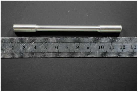
Figure 2.
Tensile specimen.
This tensile test is mainly a quasi-static stretching test. The strain rate range of the quasi-static stretching is 10−4s −1 to 10−2s−1 [,,]. According to the calculation using Equation (1), the electronic universal test can be obtained. The strain rate measurement range of the machine is 10−5s−1 to 10−1s−1. Therefore, three strain rates of 10−4s −1, 10−3s−1, and 10−2s−1 were selected for the herbal tensile test, and three sets of tests were conducted at each strain rate.
2.3. Finite Element Model
The simulation was carried out using commercial Abaqus software. The rolling head adopts a cemented carbide ball with the same size as the ball burnishing device. Since the hardness of the rolling head is far greater than that of the workpiece, the strain generated during processing could be ignored. The ball was set to be a rigid body. In the ball burnishing working conditions, the cemented carbide ball extrudes the workpiece, and the workpiece is driven by the lathe spindle to complete the ball burnishing process at the same time. In the process of model building, in order to avoid complex motion settings, the finite element model of the part to be machined adopted some assumptions of D. Shivalingappa et al. []. The contact part between the tool head and the bar was always in a tangent position, so the workpiece could be assumed to be an infinite plate, and the tool head rotated the extruded plate to complete the ball burnishing process. The finite element model size of the ball burnishing process is shown in Figure 3.
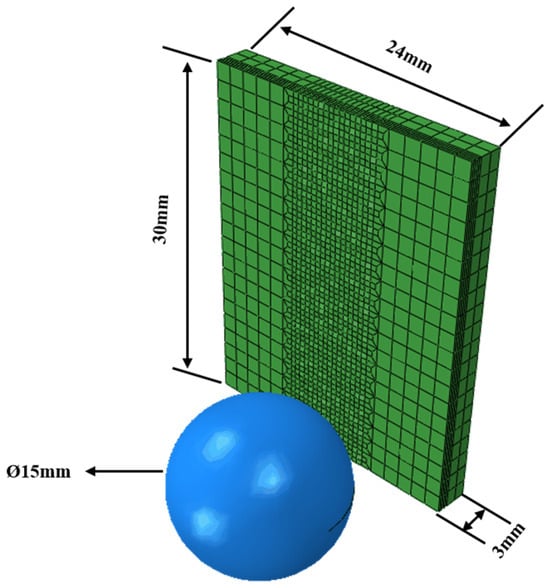
Figure 3.
The finite element model size of ball burnishing process.
The smaller the mesh, the more accurate the simulation results will be. But the large number of meshes will also cause a significant extension of the computing time, and effective meshing can reduce the computational cost without compromising accuracy. Figure 4 shows an enlarged view of the local details of a finite element mesh. Consequently, taking into account the fact that the tool head and workpiece surface were in direct contact, to increase the simulation’s accuracy, a fine mesh was used on the portion of the material surface that was in contact with the cemented carbide ball. A 1:3 transition grid was employed in the directions of X and Y to reduce the cost of the calculation time. The middle path of the plate used a Python script to set a random surface roughness. In the actual working conditions, the roughness of the material surface is at the micron level. If it is to be reflected in the model, then the mesh size needs to reach the micron level, and the overall model mesh number will reach the millions, which requires huge computational costs. In order to avoid this situation, the surface roughness randomly established by the script was Ra30.
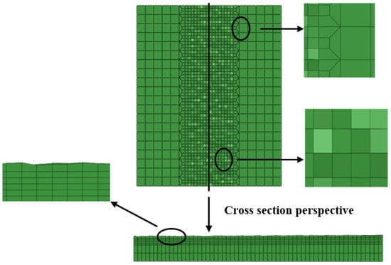
Figure 4.
The enlarged view of local details of finite element mesh.
2.4. JC Constitutive Model and Selection of Material Parameters
The JC constitutive model was first suggested by Johnson and Cook in 1983 []. The main part of the model consists of three parts: the work hardening, strain rate strengthening, and thermal softening of the material, respectively. This model can meet the requirements of simulating materials under different working conditions. The specific expression is as follows [,,,,]:
Expressions A, B, C, n, and m are the pending parameters. A, B, and n describe the material’s strain hardening properties at the reference temperature and reference strain rate, where A is the quasi-static yield strength. B is the coefficient of strain hardening, and n is the index of strain hardening. C is the strain rate constant. is the reference strain rate. is the melting point. is the reference temperature. σ is the true stress. ε is the plastic strain. is the strain rate. T is the test temperature [,,,,].
The Johnson–Cook model material parameters and compressed material parameters were employed in this simulation. The JC parameters need to be calculated and will be explained in detail below. The compressed material parameters used by Moćko et al. [] are displayed in Table 3. The data in Table 3 were used to simulate the ball burnishing process directly. The compression curve is drawn using the relationship between the stress and deformation of the material in the experiment, to ensure that it is accurate. The JC model only considers the effects of strain, strain rate, and temperature. This does not take into account the coupling effect between different factors. Therefore, in some cases, the accuracy of the model may have some problems. The stress and deformation of the material in the actual situation are one-to-one correspondences. Based on this, firstly, the stress–strain curves of the deformed mesh from the simulated ball burnishing process using compression parameters and JC parameters were extracted. The difference between the two curves was analyzed. Secondly, the JC parameters were calculated at different strain rates. Further, the way the values of the residual stress field in the simulated ball burnishing process changed when the values of the JC parameters changed were analyzed. Finally, the most appropriate JC parameter value was selected through comparison to control the residual stress field value of the ball milling and polishing simulation within a reasonable range.
Table 3.
Compression parameters for 7075-T651 aluminum alloy [].
3. Results
3.1. Ball Burnishing Experimental Results
After conducting multiple experiments to obtain the average, the residual stress test value from the ball burnishing process was determined, which is displayed in Table 4. When the static pressure was 150 N, the residual stress value was −77.43 MPa. When the static pressure was 300 N, the residual stress value was −119.87 MPa. When the residual stress was 600 N, the residual stress value was −234.87 MPa. The compressive residual stress increases with increasing static pressure.
Table 4.
Test value of residual stress in ball burnishing.
3.2. Calculation Results of the JC Model
In the ball burnishing process, the material is processed at room temperature, which is significantly below the melting point of the substance. The value of is generally room temperature. T is the temperature during the ball burnishing process, which is close to room temperature. is the melting point temperature of the material, which is much higher than room temperature. The value of the temperature term in Formula (2) is approximately equal to one. Therefore, the thermal softening effect of the material does not need to be considered, and the model can be simplified as follows []:
The ball rolling process is a quasi-static process. Here, it is = 10−3s−1. The flow stress of the material does not show changes under the quasi-static strain rate. This indicates that the effect of strain rate hardening can be ignored in the JC model, so Equation (3) is simplified to the following equation:
Figure 5 depicts the stress–strain curve obtained during the tensile experiment, which facilitates the calculation of material constants for the JC model. The A value is calculated based on the quasi-static yield stress. It can be concluded from Formula (4) that the A value is the intercept of the quasi-static yield stress fitting line. The specific values are shown in Table 5.
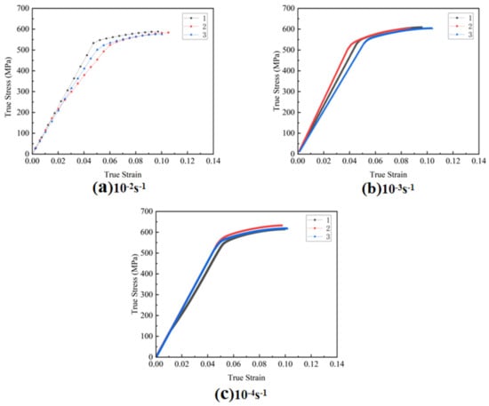
Figure 5.
Stress–strain curves at different strain rates.
Table 5.
Values of parameter A.
By applying the natural logarithm to both sides of Equation (4), the equation undergoes a transformation:
We substituted the A value and the flow stress data under various strains into Equation (5) to draw the relationship between and , as shown in Figure 6. The value of n can be determined by analyzing the slope of the fitting line obtained from the data. Additionally, the intersecting point of the fitting line with the ordinate enables the calculation of the value of B; the specific values are shown in Table 6.
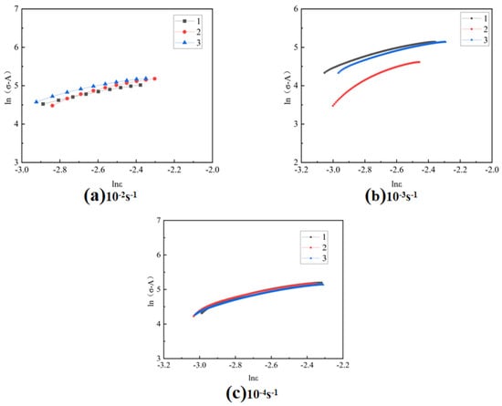
Figure 6.
Curves of and at different strain rates.
Table 6.
Values of parameters B and n at different rates.
3.3. Ball Burnishing Simulation Results
Table 3, Table 5 and Table 6 include data that were utilized to simulate the ball burnishing process under static pressures of 150 N, 300 N, and 600 N, respectively.
By hiding the burnishing ball and only showing the workpiece, we extracted the residual stress at the center node of the path and calculated the average value. Figure 7 shows the residual stress field of the compression parameters under different loading conditions: Figure 7a shows the ball burnishing simulation result under 150 N static pressure, and there was −78.23 MPa of residual stress in the ball burnishing path; Figure 7b shows the ball burnishing simulation result under 300 N static pressure, and there was −120.31 MPa of residual stress in the ball burnishing path; and Figure 7c shows the ball burnishing simulation result under 600 N static pressure, and there was −236.7 MPa of residual stress in the ball burnishing path.
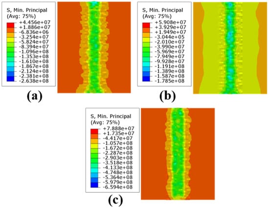
Figure 7.
Residual stress field of compression parameters under different loading conditions: (a) 150 N; (b) 300 N; (c) 600 N.
Figure 8 displays the residual stress field of the JC parameters under different loading conditions when the rate is 10−2s−1. Figure 8a displays the outcomes of the ball burnishing simulation under 150 N static pressure; the residual stress in the ball burnishing path was −73.65 MPa. Figure 8b shows the ball burnishing simulation results under 300 N static pressure; the residual stress was −136.96 MPa. Figure 8c shows the ball burnishing simulation results at 600 N static pressure; the residual stress was −236.13 MPa.
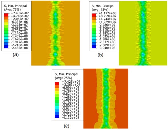
Figure 8.
Residual stress field of JC parameters under different loading conditions when the −2s−1: (a) 150 N; (b) 300 N; and (c) 600 N.
Figure 9 displays the residual stress field of the JC parameters under different loading conditions when the strain rate is 10−3s−1. Figure 9a displays the outcomes of the ball burnishing simulation under 150 N static pressure; the residual stress in the ball burnishing path was −70.33 MPa. Figure 9b shows the ball burnishing simulation results under 300 N static pressure; the residual stress was −142.32 MPa. Figure 9c shows the ball burnishing simulation results at 600 N static pressure; the residual stress was −252.14 MPa.
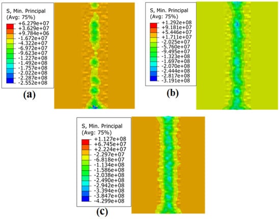
Figure 9.
Residual stress field of JC parameters under different loading conditions when the −3s−1: (a) 150 N; (b) 300 N; (c) and 600 N.
Figure 10 displays the residual stress field of the JC parameters under different loading conditions when the strain rate is 10−4s −1. Figure 10a displays the outcomes of the ball burnishing simulation under 150 N static pressure; the residual stress in the ball burnishing path was −74.29 MPa. Figure 10b shows the ball burnishing simulation results under 300 N static pressure; the residual stress was −129.51 MPa. Figure 10c shows the ball burnishing simulation results at 600 N static pressure; the residual stress was −240.91 MPa.
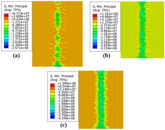
Figure 10.
Residual stress field of JC parameters under different loading conditions when the −4s−1: (a) 150 N; (b) 300 N; and (c) 600 N.
Both the simulations and the actual data of the four parameters show that when the static pressure increases, the residual stress of the material increases. The reason for this is that, when the static pressure increases, the material’s surface will undergo a greater plastic deformation.
Figure 11 shows the comparison of the simulation results using the JC parameters and compression parameters with the experimental results. The findings demonstrate that the experimental values and the simulation results under the compression parameters are essentially consistent, which could verify the accuracy of the compression parameters. The JC parameter simulation results are larger than the experimental values. The simulated results of the JC parameters are compared with the experimental results in Table 7.
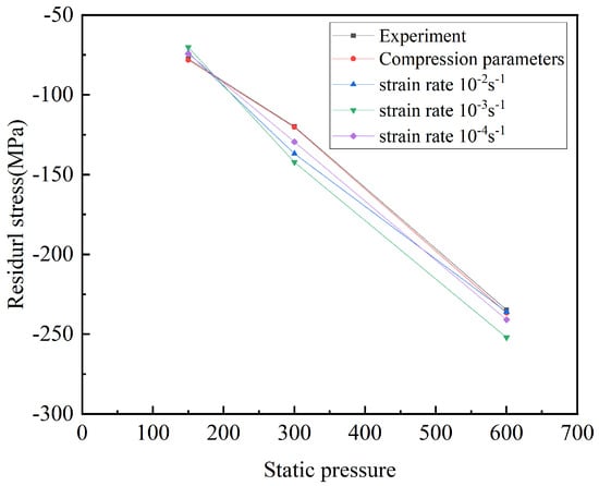
Figure 11.
Relationship between static pressure and residual stress.
Table 7.
The comparison between the simulation results of JC parameters and the experimental results.
Based on the findings, it was observed that a static pressure of 600 N yielded the most accurate fitting results when combined with a strain rate of 10−2s−1. The discrepancy or deviation in these results was minimal, measuring only 0.5%. After conducting the experiment with a static pressure of 300 N, it was determined that the strain rate of 10−4s −1 yielded the most accurate results. The deviation in these results was measured to be 8.1%. When the static pressure reaches 150 N, the optimal outcome for the strain rate of 10−4s −1 exhibits the highest level of agreement, with a discrepancy of merely 4.1%.
Figure 12 shows the stress–strain curve of a deformed mesh after the ball burnishing simulation. The findings indicated that during the elastic stage, the curves of the JC parameters and compression parameters basically coincide, and the slope of the curve in the elastic stage was consistent. The reason was that the Abaqus software has a linear relationship for the equations of the elastic phase, and the difference in this part depends mainly on the Poisson’s ratio and the modulus of elasticity. During the plastic stage, there is a difference in the stress–strain curve between the JC parameters and the compression parameters. When the curve using the compression parameters had reached the yield point, the result of the JC parameters had not yet yielded but required higher stress to produce the yield phenomenon.
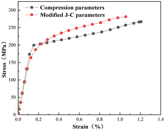
Figure 12.
Stress–strain curves of compression parameters and J-C parameters.
3.4. Surface Roughness
Surface roughness is an important indicator to measure the quality of ball burnishing; a good surface effect has always been the ultimate purpose of the ball burnishing process. As mentioned above, it is difficult to reproduce the topographic surface roughness in a numerical simulation, which requires very small meshes and therefore a huge computational cost. Therefore, by amplifying the surface roughness established in the numerical simulation to about 15 times the actual working conditions, and simulating with the adjusted JC parameters, the final surface roughness of different ball burnishing conditions was qualitatively analyzed. Surface roughness is usually expressed by Ra or Rz. Ra measures the average displacement of points from the reference line within a given sampling length, while Rz takes into account the sum of the average values of the five maximum peak heights and valley depths over the same length []. Rz is generally only used to represent relatively short surfaces because there are not many Rz measurement points; for this reason, its characteristics in reflecting the height of microscopic geometry are not as full as Ra parameters, and it does not have the characteristics of Ra that make it more precise. For the ball burnishing process, Ra was more suitable, so the measurement of roughness in the experiments was expressed by Ra.
By drawing the curve of the node coordinate changes of the ball burnishing motion path, the changes in the path after processing can be vividly represented. Figure 13 shows the path of the extracted node. We extracted the Z coordinate data of all nodes on the path before and after ball burnishing. Figure 14 shows the curve drawn by the extracted node Z coordinate data under different working conditions. The smoother the path curve, the flatter the simulated surface, and the lower the roughness value. The results showed that the path curve under the static pressure of 150 N and 300 N was smoother than the original raw path curve, and the curve became steeper when the static pressure was 600 N. The reason is that when the static pressure used is too large, the material surface will produce a large plastic deformation, and the material’s surface may be crushed. The smoothest path curve was obtained at a static pressure of 300 N.
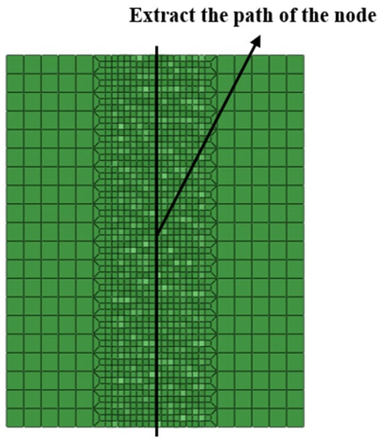
Figure 13.
Extracted Z coordinate data of all nodes on the path.
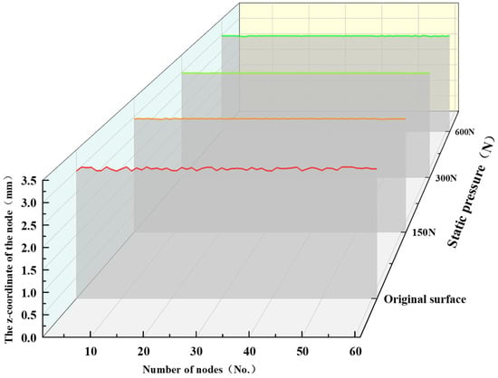
Figure 14.
Node coordinates under different working conditions.
Figure 15 shows the relationship curve between the surface roughness and static pressure; Figure 15a is the simulated value, and Figure 15b is the experimental value. The results showed that the Ra steadily diminished as the static pressure increased between 0–300 N, and under a static pressure of 600 N, the Ra tended to increase. During the process of ball burnishing, the tool head transfers static pressure to the rotating mechanical parts’ surfaces, resulting in the impact extrusion effect, which makes the metal material produce a large elastic–plastic deformation. After processing, on the surface of the workpiece, there was a certain elastic recovery, and the subsequent plastic flow flattens the surface of the workpiece’s minuscule wave peak. When the static pressure was low, the energy required for the metal flow cannot fully meet the flow of metal to the valley. When the static pressure was properly increased, the roughness value would decrease accordingly. However, when the static pressure was too high, the energy would overflow, and excessive static pressure would lead to increased friction on the contact surface. The surface of the material would be crushed, the metal would peel, and the surface quality would deteriorate. The comparison of the simulation and experimental results showed that the variation trend of surface roughness is consistent. There was a significant difference between the simulation results and experimental results in terms of surface roughness values. This is because the original surface roughness established in the finite element model was greater than the surface roughness during the actual machining process. As mentioned earlier, it is difficult to establish the same original surface roughness in the finite element model as in the actual machining process, and it is only possible to establish the original surface roughness as close as possible to the actual machining process. Therefore, the original surface roughness established in the finite element model was approximately 15 times that of the actual machining process.
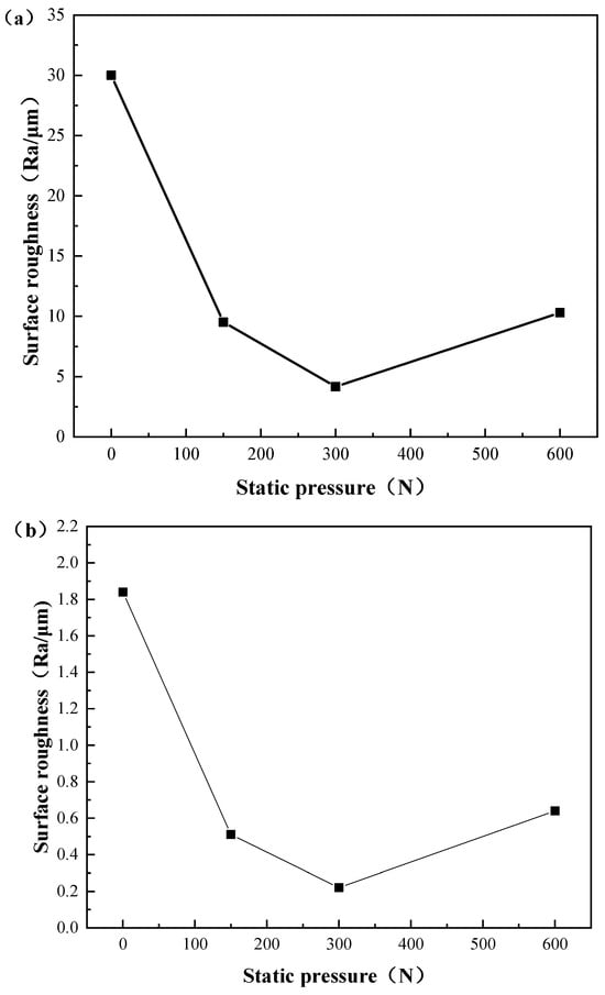
Figure 15.
Relationship between surface roughness and static pressure: (a) numerical simulation results and (b) experimental results.
4. Conclusions
Based on the Abaqus simulation software, the Johnson–Cook constitutive model parameters and compression parameters were selected to simulate the ball burnishing process of the 7075-T651 aluminum alloy. A method for adjusting Johnson–Cook parameters was proposed. The error between the numerical simulation results adjusted using this method and the experimental results was within 10%. The main conclusions of this article are as follows:
- A method for adjusting Johnson–Cook parameters has been proposed, which is suitable for low strain rate machining simulations. Through tensile experiments, we calculated the JC parameters corresponding to different strain rates under quasi-static conditions and used Abaqus simulation software to simulate and calculate the corresponding residual stress field. Through a comparative analysis, it was found that the ball polishing simulation results of the JC parameters calculated at a strain rate of 10−4s −1 maintained the error between the experimental results within 10%.
- A simulation comparison method was proposed to compare the stress–strain curves of the JC parameters calculated by the numerical simulation with the compression parameters. It was found that there is a similar development trend in the elastic and plastic stages, further verifying the accuracy of the Johnson–Cook parameters and the feasibility of the method.
- A method for simulating surface roughness was proposed, using improved Johnson–Cook parameters for ball polishing simulations and characterizing surface roughness. The results indicate that the simulated surface roughness has a consistent trend with the experimental values. In the range of 0–300 N, the Ra gradually decreases with the increase of static pressure. Under a static pressure of 600 N, the Ra increases due to the crushing of the material surface.
In this study, a method to modify the parameters of the JC model was proposed to make it suitable for simulating low strain rate machining processes such as ball burnishing, which supports subsequent simulation studies of ball burnishing processes. This method mainly adjusts JC parameters by means of numerical simulation, which reduces experimental research.
Author Contributions
Conceptualization, Y.C., J.C. and Y.W.; methodology, Y.W. and J.C.; software, J.C. and X.W.; writing–original draft, D.Y. and H.Z.; writing–review and editing, D.Y. and H.Z.; formal analysis, Y.W. All authors have read and agreed to the published version of the manuscript.
Funding
The authors acknowledge the support from the National Natural Science Foundation of China (No. U1904185), Henan Province Science and Technology Research (232102521022) and The Henan Province college youth backbone teacher (2020GGJS071).
Data Availability Statement
The data presented in this study are available on request from the corresponding author. The data are not publicly available due to privacy reasons.
Acknowledgments
Special thanks to Keke Zhang and Xiao Xiao from School of Materials Science and Engineering, Henan University of Science and Technology, Luoyang China for their assistance in analyzing the data in this article.
Conflicts of Interest
The authors declare no conflict of interest.
References
- Dursun, T.; Soutis, C. Recent Developments in Advanced Aircraft Aluminium Alloys. Mater. Des. (1980–2015) 2014, 56, 862–871. [Google Scholar] [CrossRef]
- Klocke, F.; Liermann, J. Roller Burnishing of Hard Turned Surfaces. Int. J. Mach. Tools Manuf. 1998, 38, 419–423. [Google Scholar] [CrossRef]
- Zhang, P.; Lindemann, J.; Ding, W.J.; Leyens, C. Effect of Roller Burnishing on Fatigue Properties of the Hot-Rolled Mg–12Gd–3Y Magnesium Alloy. Mater. Chem. Phys. 2010, 124, 835–840. [Google Scholar] [CrossRef]
- Yuan, X.L.; Sun, Y.W.; Gao, L.S.; Jiang, S.L. Effect of Roller Burnishing Process Parameters on the Surface Roughness and Microhardness for TA2 Alloy. Int. J. Adv. Manuf. Technol. 2016, 85, 1373–1383. [Google Scholar] [CrossRef]
- Buldum, B.B.; Cagan, S.C. Study of Ball Burnishing Process on the Surface Roughness and Microhardness of AZ91D Alloy. Exp. Tech. 2018, 42, 233–241. [Google Scholar] [CrossRef]
- Rodríguez, A.; López de Lacalle, L.N.; Celaya, A.; Lamikiz, A.; Albizuri, J. Surface Improvement of Shafts by the Deep Ball-Burnishing Technique. Surf. Coat. Technol. 2012, 206, 2817–2824. [Google Scholar] [CrossRef]
- Hilpert, M.; Wagner, L. Corrosion Fatigue Behavior of the High-Strength Magnesium Alloy AZ 80. J. Mater. Eng. Perform. 2000, 9, 402–407. [Google Scholar] [CrossRef]
- Zhang, P.; Lindemann, J. Effect of Roller Burnishing on the High Cycle Fatigue Performance of the High-Strength Wrought Magnesium Alloy AZ80. Scr. Mater. 2005, 52, 1011–1015. [Google Scholar] [CrossRef]
- El-Axir, M.H. An Investigation into Roller Burnishing. Int. J. Mach. Tools Manuf. 2000, 40, 1603–1617. [Google Scholar] [CrossRef]
- El-Khabeery, M.M.; El-Axir, M.H. Experimental Techniques for Studying the Effects of Milling Roller-Burnishing Parameters on Surface Integrity. Int. J. Mach. Tools Manuf. 2001, 41, 1705–1719. [Google Scholar] [CrossRef]
- Barahate, V.; Govande, A.R.; Tiwari, G.; Sunil, B.R.; Dumpala, R. Parameter Optimization during Single Roller Burnishing of AA6061-T6 Alloy by Design of Experiments. Mater. Today Proc. 2022, 50, 1967–1970. [Google Scholar] [CrossRef]
- Yen, Y.C.; Sartkulvanich, P.; Altan, T. Finite Element Modeling of Roller Burnishing Process. CIRP Ann. 2005, 54, 237–240. [Google Scholar] [CrossRef]
- Sartkulvanich, P.; Altan, T.; Jasso, F.; Rodriguez, C. Finite Element Modeling of Hard Roller Burnishing: An Analysis on the Effects of Process Parameters Upon Surface Finish and Residual Stresses. J. Manuf. Sci. Eng. 2007, 129, 705–716. [Google Scholar] [CrossRef]
- Balland, P.; Tabourot, L.; Degre, F.; Moreau, V. Mechanics of the Burnishing Process. Precis. Eng. 2013, 37, 129–134. [Google Scholar] [CrossRef]
- Zhang, D.; Zhang, X.-M.; Ding, H. Experimental and Numerical Study of the Subsurface Deformation and Residual Stress during the Roller Burnishing Process. Procedia CIRP 2020, 87, 491–496. [Google Scholar] [CrossRef]
- Duncheva, G.V.; Maximov, J.T.; Anchev, A.P.; Dunchev, V.P.; Atanasov, T.P.; Capek, J. Finite Element and Experimental Study of the Residual Stresses in 2024-T3 Al Alloy Treated via Single Toroidal Roller Burnishing. J. Braz. Soc. Mech. Sci. Eng. 2021, 43, 55. [Google Scholar] [CrossRef]
- Rotella, G.; Saffioti, M.R.; Sanguedolce, M.; Umbrello, D. Finite Element Modelling of Combined Turning/Burnishing Effects on Surface Integrity of Ti6Al4V Alloy. Int. J. Adv. Manuf. Technol. 2022, 119, 177–187. [Google Scholar] [CrossRef]
- Borysenko, D.; Welzel, F.; Karpuschewski, B.; Kundrák, J.; Voropai, V. Simulation of the Burnishing Process on Real Surface Structures. Precis. Eng. 2021, 68, 166–173. [Google Scholar] [CrossRef]
- McCarthy, M.A.; Xiao, J.R.; McCarthy, C.T.; Kamoulakos, A.; Ramos, J.; Gallard, J.P.; Melito, V. Modelling of Bird Strike on an Aircraft Wing Leading Edge Made from Fibre Metal Laminates—Part 2: Modelling of Impact with SPH Bird Model. Appl. Compos. Mater. 2004, 11, 317–340. [Google Scholar] [CrossRef]
- Sahu, S.; Mondal, D.P.; Goel, M.D.; Ansari, M.Z. Finite element analysis of AA1100 elasto-plastic behaviour using Johnson-Cook model. Mater. Today Proc. 2018, 5, 5349–5353. [Google Scholar] [CrossRef]
- Tan, J.Q.; Zhan, M.; Liu, S.; Huang, T.; Guo, J.; Yang, H. A Modified Johnson–Cook Model for Tensile Flow Behaviors of 7050-T7451 Aluminum Alloy at High Strain Rates. Mater. Sci. Eng. A 2015, 631, 214–219. [Google Scholar] [CrossRef]
- Zhao, Y.; Sun, J.; Li, J.; Yan, Y.; Wang, P. A Comparative Study on Johnson-Cook and Modified Johnson-Cook Constitutive Material Model to Predict the Dynamic Behavior Laser Additive Manufacturing FeCr Alloy. J. Alloys Compd. 2017, 723, 179–187. [Google Scholar] [CrossRef]
- Niu, L.; Cao, M.; Liang, Z.; Han, B.; Zhang, Q. A Modified Johnson-Cook Model Considering Strain Softening of A356 Alloy. Mater. Sci. Eng. A 2020, 789, 139612. [Google Scholar] [CrossRef]
- Wang, Y.; Zeng, X.; Chen, H.; Yang, X.; Wang, F.; Zeng, L. Modified Johnson-Cook Constitutive Model of Metallic Materials under a Wide Range of Temperatures and Strain Rates. Results Phys. 2021, 27, 104498. [Google Scholar] [CrossRef]
- Teimouri, R.; Amini, S.; Guagliano, M. Analytical Modeling of Ultrasonic Surface Burnishing Process: Evaluation of Residual Stress Field Distribution and Strip Deflection. Mater. Sci. Eng. A 2019, 747, 208–224. [Google Scholar] [CrossRef]
- Liu, Z.; Zhao, H.; Li, J.; Niu, Z.; Ji, V. Modified Johnson–Cook Constitutive Model of 18CrNiMo7-6 Alloy Steel under Ultrasonic Surface Burnishing Process. J. Mater. Eng. Perform. 2022, 32, 4022–4030. [Google Scholar] [CrossRef]
- GB/T 16865-2013; Test Pieces and Method for Tensile Test for Wrought Aluminium and Magnesium Alloys Products. Standardization Administration of the People’s Republic of China: Beijing, China, 2013.
- Zhang, D.N.; Shangguan, Q.Q.; Xie, C.J.; Liu, F. A modified Johnson–Cook model of dynamic tensile behaviors for 7075-T6 aluminum alloy. J. Alloys Compd. 2015, 619, 186–194. [Google Scholar] [CrossRef]
- Meng, H.; Li, Q.M. Correlation between the accuracy of a SHPB test and the stress uniformity based on numerical experiments. Int. J. Impact Eng. 2003, 20, 537–555. [Google Scholar] [CrossRef]
- He, Z.; He, Y.; Ling, Y.; Wu, Q.; Gao, Y.; Li, L. Effect of strain rate on deformation behavior of TRIP steels. J. Mater. Process. Technol. 2012, 212, 2141–2147. [Google Scholar] [CrossRef]
- Harish; Shivalingappa, D.; Raghavendra, N.; Ganesh, V. Impact of Ball Burnishing Process on Residual Stress Distribution in Aluminium 2024 Alloy Using Experimental and Numerical Simulation. IOP Conf. Ser. Mater. Sci. Eng. 2021, 1189, 012002. [Google Scholar] [CrossRef]
- Xie, H.; Zhang, X.; Miao, F.; Jiang, T.; Zhu, Y.; Wu, X.; Zhou, L. Separate Calibration of Johnson-Cook Model for Static and Dynamic Compression of a DNAN-Based Melt-Cast Explosive. Materials 2022, 15, 5931. [Google Scholar] [CrossRef] [PubMed]
- Priest, J.; Ghadbeigi, H.; Ayvar-Soberanis, S.; Liljerehn, A.; Way, M. A Modified Johnson-Cook Constitutive Model for Improved Thermal Softening Prediction of Machining Simulations in C45 Steel. Procedia CIRP 2022, 108, 106–111. [Google Scholar] [CrossRef]
- Ben Said, L.; Chabchoub, A.K.; Wali, M. Mathematical Model Describing the Hardening and Failure Behaviour of Aluminium Alloys: Application in Metal Shear Cutting Process. Mathematics 2023, 11, 1980. [Google Scholar] [CrossRef]
- Shen, X.; Zhang, D.; Yao, C.; Tan, L.; Li, X. Research on Parameter Identification of Johnson–Cook Constitutive Model for TC17 Titanium Alloy Cutting Simulation. Mater. Today Commun. 2022, 31, 103772. [Google Scholar]
- Moćko, W.; Rodríguez-Martínez, J.A.; Kowalewski, Z.L.; Rusinek, A. Compressive Viscoplastic Response of 6082-T6 and 7075-T6 Aluminium Alloys Under Wide Range of Strain Rate at Room Temperature: Experiments and Modelling. Strain 2012, 48, 498–509. [Google Scholar] [CrossRef]
- Murugesan, M.; Jung, D.W. Johnson Cook Material and Failure Model Parameters Estimation of AISI-1045 Medium Carbon Steel for Metal Forming Applications. Materials 2019, 12, 609. [Google Scholar] [CrossRef]
- Kadivar, M.; Tormey, D.; McGranaghan, G. A Review on Turbulent Flow over Rough Surfaces: Fundamentals and Theories. Int. J. Thermofluids 2021, 10, 100077. [Google Scholar] [CrossRef]
Disclaimer/Publisher’s Note: The statements, opinions and data contained in all publications are solely those of the individual author(s) and contributor(s) and not of MDPI and/or the editor(s). MDPI and/or the editor(s) disclaim responsibility for any injury to people or property resulting from any ideas, methods, instructions or products referred to in the content. |
© 2023 by the authors. Licensee MDPI, Basel, Switzerland. This article is an open access article distributed under the terms and conditions of the Creative Commons Attribution (CC BY) license (https://creativecommons.org/licenses/by/4.0/).