Abstract
Additive manufacturing (AM) simulations are effective for materials that are well characterized and published; however, for newer or proprietary materials, they cannot provide accurate results due to the lack of knowledge of the material properties. This work demonstrates the process of the application of mathematical search algorithms to develop an optimized material dataset which results in accurate simulations for the laser directed energy deposition (DED) process. This was performed by first using a well-characterized material, Ti-64, to show the error in the predicted melt pool was accurate, and the error was found to be less than two resolution steps. Then, for 7000-series aluminum using a generic material property dataset from sister alloys, the error was found to be over 600%. The Nelder–Mead search algorithm was then applied to the problem and was able to develop an optimized dataset that had a combined width and depth error of just 9.1%, demonstrating that it is possible to develop an optimized material property dataset that facilitates more accurate simulation of an under-characterized material.
1. Introduction
Additive manufacturing (AM) is an emerging manufacturing technique that has the potential to revolutionize manufacturing. To realize this revolution, it is necessary to be able to produce components reliably and to understand the process well enough to ensure that builds are consistent enough that the performance of the completed build can be guaranteed. To execute this, researchers and manufacturers have turned to mathematical modeling to understand the process [1]. This body of work focuses solely on increasing the accuracy of thermal modeling of the process; however, the thermal cycling that a build experiences affects the resulting microstructure [2,3,4], residual stress and distortion [3,5,6], and porosity of the build [7,8,9]. If the accuracy of the underlying thermal modeling prediction can be improved, then the subsequent properties can be more accurately modeled as well.
The differences in simulation techniques can vary based on the desired response from the simulation and the underlying assumptions that were made during the development of the models. One example of this can be seen when comparing the mathematical models developed by Wang and Chen [10], Roy and Wodo [11], and Moges et al. [12]. They all attempted to model roughly the same aspect of the build but took very different approaches. Wang and Chen [10] took a purely physics-based approach to the solution and developed a model from a fundamental physics-first principle approach for the physical process being modeled. This was performed for Ti-64 and was able to obtain an accuracy of between 3.6% and 9.0%. On the contrary, Roy and Wodo [11] used a data-driven model that used a breadth of data to develop a mathematical model that properly predicted the material behavior. This model was applied to the plastic fused filament fabrication (FFF) process due to the volume of data required. It would be possible to develop the model for a metal process, though it could become cost-prohibitive quickly. In between these models exists Moges et al. [12], which attempted to marry the two approaches and develop a physics-based model that uses data to improve the accuracy. This was able to produce results with an average relative error of 7.58% for Inconel 625.
The one unifying characteristic of these, and all mathematical models, is the need for the inclusion of a dataset that defines the behavior of the material being investigated; this is colloquially referred to as the material properties. These material properties can vary in the literature and this variance in values can lead to a discrepancy in simulation results [13]. This need for input material properties extends to surrogate models that have been developed, such as machine learning (ML) models, which will also require the inclusion of these material properties to properly predict the outcome [14,15,16,17].
Though variation exists in the literature, values can be found and used when the material is well characterized and published. An example of a well-published material is Ti-64, where it is easy to find literature that reports the material properties such as Welsch et al. [18], Boivineau et al. [19], and Fan and Liou [20]. However, for materials that are not well characterized or published, such as specific aluminum alloys, it can be very challenging to find some properties, as reported by Lindberg [21] and Leitner et al. [22]. There arises a need to determine a complete dataset of the material properties, or at a minimum, develop a dataset that produces the most accurate simulation results. This can be accomplished by expending the necessary resources to measure the needed properties using advanced equipment. This process can be expensive and time-consuming, which has led to the development of material simulations that attempt to predict the material properties, such as JMatPro [23]. Though faster and cheaper than experimental results, they, like all simulations, have an error that is associated with them; this has been reported by Liu et al. [24], Chen et al. [25], and Geng et al. [26]. Using these values alone can lead to unknown errors stacking up in the additive manufacturing (AM) models. This problem also applies to materials where the tolerances for alloying elements is so wide that specimens of the same alloy can have different material properties.
To develop a dataset that produces accurate AM simulation results, an optimization routine can be used as a search algorithm to determine the dataset that produces the most realistic results. This can be used to develop a dataset for a new alloy or for a specific batch of stock that has been procured from a supplier.
This work will aim to address one of the current desires in metal AM which is to be able to produce parts out of aluminum. The desire is evident by the volume of effort being applied to aluminum AM [27,28,29]. The challenge associated with this stems from the wide range of alloys that have wildly varying material properties and are not well published. One of the weldable high-strength alloys that have been targeted for metal AM is 7050 [30]. Though the material is widely available, the temperature-dependent material properties are not readily available. This work will perform an optimization routine on the material dataset for the 7050 aluminum alloy to enable more accurate simulation results. This will be performed by validating the model on the well-characterized Ti-64 material, showing the model’s effectiveness. Then, utilizing sister alloys, a generic material property dataset will be found in the literature. The search algorithm will then be applied to generate an optimal input property dataset. These optimized material properties will then be used with a range of laser parameters and compared experimentally to show their effectiveness over a processing window.
2. Materials and Methods
This body of work begins by describing the thermal model which was developed to simulate the metal AM deposition process for any metal where the material properties could be determined. This model is then validated using a well-characterized material, Ti-64. Upon validation of the thermal model, it is applied to a generic aluminum alloy, and then experimentation is used to determine if the results are a good representation of the physical process. When found to be inaccurate, a mathematical search algorithm was applied to the input parameters to increase the accuracy of the model’s results. Lastly, the optimal input dataset was validated by comparing the simulated results to experimental results with a range of laser scan speeds and power levels for the targeted aluminum alloy.
2.1. Simulation Description
The model used in this study was developed at the Missouri University of Science and Technology. This simulation has the express goal of being efficient while still holding to physics models. To accomplish this, it heavily leverages GPU processing by utilizing image processing techniques. The simulation was developed with the laser DED processes in mind; however, it was developed in a modular manner such that it can be applied to most AM processes.
The model is a voxel-based simulation, which forgoes the calculation of the fluid flow and focuses on heat transfer and material insertion. This decision was based on past simulation development experience, where it was determined that the calculation of the fluid flow was the most computationally expensive part of the simulation.
The governing equations of the model developed can be seen in Equations (1)–(3), which describe the flow of heat from conduction, convection, and radiation, and laser absorption, respectively [31].
In these equations, is density, is specific heat, k is thermal conductivity, h is convection coefficient, is emissivity, is the Stefan–Boltzmann constant, and n is the unit (outward) normal vector of a point at location that is located on the outer surface of the component, is the radius of the laser beam, is the absorption of the material with respect to the laser radiation, is the surface temperature, is the ambient temperature, is the laser power, and is a step function which is 1 for the node with the largest z value in every () location and 0 elsewhere.
The main attributes of the model are its ability to predict the thermal history of a part (Figure 1a), the phase map of the part at any given time (Figure 1b), and a cooling rate for any section of the part (Figure 1c). This helps to give a predictor of the microstructure within the deposition, which is the driving force behind the final mechanical properties.
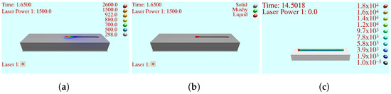
Figure 1.
Examples of data maps which can be expected from the simulation. (a) Temperature profile; (b) phase map; (c) cooling rate map.
Additionally, the laser in the simulation is modeled in 3D to be able to take into account the beam quality using the beam parameter product (BPP) reported by the manufacturer and shown in Equation (4), where and are the divergence angle and the beam waist respectively.
Lastly, the model includes true ray tracing, enabling shadowing of the laser, the ability to define a mass that represents the machine acting as a heat sink during the build process, and the inclusion of temperature-dependent material properties.
The main objective of the model is to accurately predict the thermal history of the build. To initially validate the models, the well-characterized and published material Ti-64 was used. The validation was performed by scanning a laser on the surface of a substrate at three energy densities with the experimental parameters found in Table 1, and the material properties used in the simulations can be seen in Table 2.

Table 1.
Simulation parameters used in Ti-64 validation.
Table 2.
Ti-64 material properties used in validation.
There are several representations of the energy density of a laser beam in AM, but the most appropriate method of calculating the energy for the DED process is to use the surface energy density, Equation (5), where P is laser power, A is the laser spot area, and v is the scan speed [33].
To analyze the results, the samples from the three different parameter sets were sectioned using a wire electrical discharge machine (EDM), polished using an automated polisher to a mirror finish, and etched using Kroll’s reagent to make the melt track visible with an optical microscope, as can be seen in Figure 2a, this was performed at three points along the melt length.
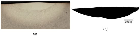
Figure 2.
Analysis of sliced sample in Ti-64 validation. (a) Sample image of the etched slice; (b) melt pool extracted from etched slice.
The experiment and simulation were compared, and the resulting error for the width can be seen in Figure 3a and that of the depth can be seen in Figure 3b.
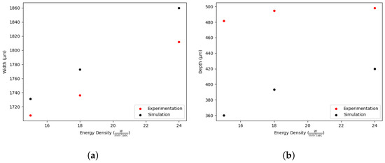
Figure 3.
Comparison of simulation and experimentation in Ti-64 validation. (a) Width; (b) Depth.
The average values that are reported on the graph have an associated standard deviation of 0.62 m, 13.7 m, and 7.74 m for the width measurements for the energy densities of 15 , 18 , and 24 , respectively. For the track depth, the standard deviations are 70.2 m, 113.7 m, and 13.7 m for the energy densities of 15 , 18 , and 24 , respectively.
From the plots, it can be seen that the simulation is capable of predicting the width with an error of less than 3%, and the depth error is between 15% and 25%. The error in the width is very acceptable, at less than 3%. However, the error in the depth is larger due to the resolution (voxel size) of the simulation chosen and its size relative to the depth. This error, of approximately 20%, for the depths which range from 450–500 m is 1.3–1.7 times the resolution, 60 m, of the simulation. Since the trends of the simulation and experimentation match and the error is within two resolution distances, the 20% error in the depth is considered acceptable as well. This shows that the mathematical models developed are accurate and if the material property is well characterized, the simulation will produce accurate results.
2.2. Search Algorithm Description
The search algorithm chosen was the Nelder–Mead search algorithm [34]. This method was selected because it is one of the most popular direct search methods for the minimization of functions. The Nelder–Mead approach is a local optimization search that does not rely on the knowledge of the gradient to select the next search point. This is critical for the application of simulation results because the gradient is unknown and finding it would involve running a large number of simulations. With simulation times that can reach into days long, this is a critical consideration. Instead of knowing the actual function, it relies on n + 1 vertices. This results in a smaller number of simulation runs being needed to perform the minimization [35]. The flow chart in Figure 4 is the flow that is used to determine the next search point.
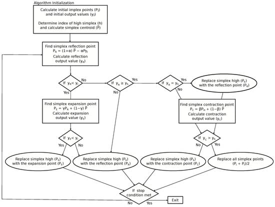
Figure 4.
Flow chart for the Nelder–Mead search algorithm.
The search begins by calculating the reflection point using Equation (6), where is the reflection coefficient.
If this reflection point is smaller than the smallest current simplex value, then the expansion is calculated using Equation (7), where is the expansion coefficient.
If the expansion point is smaller than the reflection point, then the expansion point is used to replace the largest simplex member. Otherwise, if the reflection point is larger than the expansion point, the reflection point is used to replace the largest member of the simplex, and the algorithm is restarted. If the reflection point is larger than the smallest simplex point and smaller than the second-largest point, then the highest point of the simplex is replaced with the reflection, and the algorithm is restarted. If the reflection point is between the simplex highest value and the second-highest value, a contraction is calculated, using Equation (6), with the highest values being replaced with the reflection. Otherwise, the contraction is calculated with the original simplex, still using Equation (6), where is the contraction coefficient.
If the contraction point is smaller than the largest point of the simplex, then the contraction replaces the largest point and the algorithm is continued. However, if the contraction point is larger than the highest point, a shrink step is performed, detailed in Equation (9), where is the shrink coefficient and the algorithm is restarted.
2.3. Selection of Properties
One of the attractive characteristics of the Nelder–Mead search algorithm is its ability to scale to an unlimited number of unknowns. The main adverse effects of the scaling are the increased number of runs and the combination of the errors. As the number of unknowns increases, the complexity of the search space increases, which in turn increases the number of iterations needed to find a minimum. This can result in drastically longer wait times for the search results. Additionally, with the increased number of unknowns, the stop condition of the search algorithm will be met at a different interval since the stop condition is based on the variance in the simplex. This may result in modifications to the stop conditions being necessary as a larger number of unknowns are included. If the response variable is properly defined, it will not affect the model’s results if more unknowns are included [35].
To reduce the complexity of the search algorithm, a sensitivity analysis was performed. This work began by finding the material properties that were needed in the models, as summarized in Table 3.
Table 3.
Key material properties in thermal modeling of AM.
These properties were varied according to a Placket–Burman design experiment to determine the properties which, when changed, had a statically significant effect on the resulting melt pool width, depth, and volume, as measured in Figure 5.
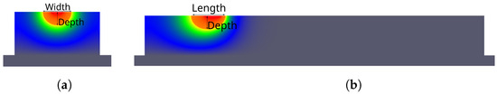
Figure 5.
Example measurements of the melt pool. (a) Width; (b) length.
Analyzing these results with Pareto charts of the standardized effects of the variables and partial regression plots of the residuals it was determined that the variables in Table 4 had a statically significant effect on the resulting melt track when modified.
Table 4.
Critical material properties.
This work included the laser diameter in the search algorithms dataset due to the difficulty associated with accurately measuring the diameter, this process is detailed in [44].
2.4. Parameter Search and Simulation Setup
For this study, the Nelder–Mead search algorithm parameters that were used can be seen in Table 5.
Table 5.
Nelder–Mead algorithm parameters.
These parameters were chosen because they fell within the guidelines of the algorithm description and after trial and error produced the most efficient searching [34].
The initial parameter values that were used as the starting point for the search algorithm can be seen in Table 6. These values were chosen based on the values that were found in the literature for similar aluminum alloys. The laser diameter was chosen based on the measuring of a melt track width on a substrate.
Table 6.
Generic aluminum material properties found in the literature.
To ensure the search algorithm did not waste time searching in unacceptable regions, the constraint was included that none of the material properties were allowed to become negative. This was the only constraint that was needed in addition to the inherent constraints of the Nelder–Mead algorithm.
The experimental setup that was used was a simple laser scanning of the surface of a substrate, as shown in Figure 6, with the parameters shown in Table 7. This was chosen to simplify the experiment. This setup removes the complexity associated with adding material, which includes the rate of material addition, molten metal flow parameters, and acceleration effect associated with turning during deposits.
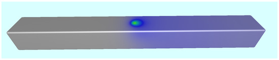
Figure 6.
Example of simulation setup used to determine melt track size.
Table 7.
Experimental constants used in search algorithm experiments.
2.5. Simulation Analysis
Upon completion of each simulation run, the saved data files were analyzed to determine the regions of the simulation that had melted. This was performed by developing a map that marked the locations of the domain that had ever been in the fluid phase. This map was then used to determine the width and depth of the melt track along the scan length, excluding the beginning and end, where effects from starting and stopping motion would affect the results. These width and depth measurements along the scan length were averaged to develop a single measurement that could be compared to the experimentation.
The experimental results were similarly determined; however, instead of a continuous set of measurements, there were four discrete measurements. These were obtained by slicing the substrate at the prescribed locations using a wire EDM. These slices were polished using an automatic polishing machine up to a mirror finish and etched using Keller’s reagent to make the microstructural differences visible by an optical microscope; an example of this can be seen in Figure 7, where the dark region had been melted during the experimentation.
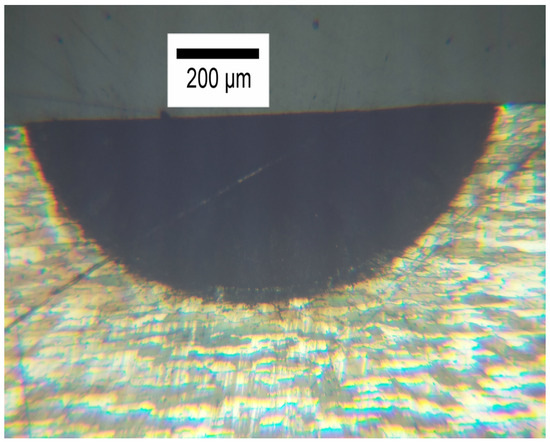
Figure 7.
Example of sliced, polished, and etched slice from aluminum experimentation.
For the Nelder–Mead search to function properly, a response variable needed to be defined. This function needed to characterize the accuracy of the simulation into a single parameter which could be minimized and upon minimization would result in the most accurate simulation. To accomplish this goal, Equation (10) was developed. This equation takes into account the error in the width of the simulation along with the error in the depth. This equation results in a non-negative number where 0 represents a simulation that perfectly matched experimentation.
3. Results
3.1. Search Algorithm Results
The search algorithm was allowed to search the space to determine the best material properties. The resulting response variables can be found in Figure 8, where the blue circular markers indicate material datasets that developed a melt track and the red diamond markers did not have the energy density to produce a melt track.
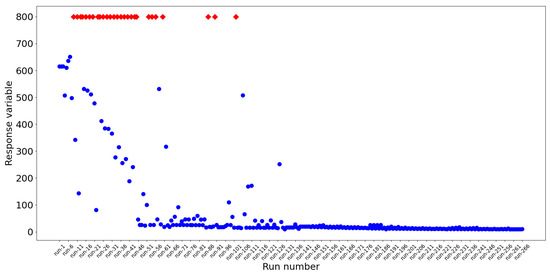
Figure 8.
Response variable of the search algorithm for material properties and laser diameter, where the blue circle marks developed a melt track and the red diamonds did not.
Due to the vast difference in scale of the initial responses and the final response variables, a new plot, Figure 9, was created, which has a max Y value of just over 30. In this plot, the blue circular markers have a response variable less than 30, the green triangle markers are those that completed with a melt track but had response variables greater than 30, and the red diamond markers are those that did not produce a melt track.
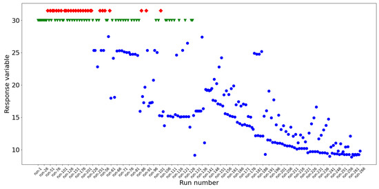
Figure 9.
Response variable of the search algorithm for material properties and laser diameter with max y axis value of 30 where the blue circle marks developed a melt track, green triangles developed a melt pool but had a response greater than 30, and red diamonds did not develop a melt pool.
In addition to these plots, the error in the width and depth were plotted and can be seen in Figure 10. In these plots, it can be seen that the error in the width is 8.83% and the error in the depth is 0.03%. It is not fully understood why all the error is coming from the width; however, it is theorized that this is a product of the difference in the size of the width vs. the depth, since the width is nearly triple that of the depth.
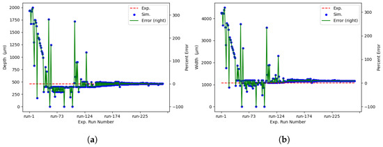
Figure 10.
Error in the individual runs of the simulations during the search algorithm. (a) Melt track depth; (b) melt track width.
The search algorithm completed and reduced the combined error from over 600% when starting from the material properties found in the literature for the generic aluminum material properties, found in Table 6, to 9.1% when using the values found in Table 8.
Table 8.
Optimized aluminum material properties and laser diameter dataset for the developed simulation.
3.2. Search Results Validation
To ensure that the search algorithm results were valid across laser travel speeds and power levels, a range of eight other parameters were compared with the experimental results. These experiments and simulations were set up and analyzed in the same manner as the search algorithm experimental setup. The base experimental parameters can be seen in Table 7, with the scan speed and laser power being varied as seen in Table 9 and the simulation material properties were used from Table 8.
Table 9.
Laser processing parameters validation processing parameters.
These speeds and powers were first completed with the literature-determined values in Table 6, and the results can be seen in Figure 11.
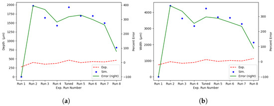
Figure 11.
Comparison of experimental and simulated results for validation points with generic literature values for the aluminum material dataset. (a) Melt track depth; (b) melt track width.
Where the red dashed line is the experimental results, the blue dots are the simulation predictions, and the green line is the error when comparing the simulated results to the experimental results. These results show that over the nine initial parameter sets, when a melt track was developed, the average absolute value of the error in the depth was approximately 290%, and the average error in the width was approximately 265%. To put this into terms of the response variable of the search algorithm, the sum of the width and depth error would be 555% combined error. Additionally, the first run was unable to develop a melt pool, which is contrary to the experiments where all the parameter sets had a stable melt track. These results corroborate the results of Figure 8, which showed that the initial dataset of material properties found in the literature is wholly inadequate for simulating the process at hand.
In contrast to these results, the material dataset found in Table 8 was used to simulate each parameter set, and the results can be seen in Figure 12.
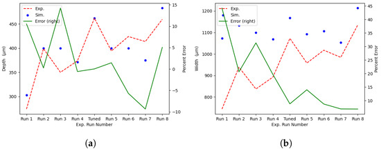
Figure 12.
Comparison of experimental and simulated results for laser processing parameter validation points with optimized values for the aluminum material dataset. (a) Melt track depth; (b) melt track width.
Where the red dashed line is the experimental results, the blue dots are the simulation predictions, and the green line is the error when comparing the simulated results to the experimental results. These results show the average error in the width was approximately 17% and the average error in the depth was approximately 5%, which creates a combined error of only 22%. These results show that the optimized dataset is better at predicting the combined error of the simulation by over 500%. This results in a simulation that can be leveraged more intensely during the process development and build qualification process. These results are from a wide parameter set that encompasses most of the usable parameter space for the deposition found experimentally. This improvement in accuracy will allow for greater application of the model in the determination of an optimized parameter set for a given build. In addition, the model is seen to be more accurate at parameters above the parameter used during the optimization. This leads to the conclusion that if a more accurate simulation is needed, the optimization should be conducted at a parameter set near the desired parameter set.
4. Discussion
After the simulation developed was shown to properly model the laser DED process for a material where the material properties were known, Ti-64, it was understood that the model held to the fundamental physics equations which the model was developed upon and any assumptions in the model were accurate enough to produce accurate results. This was detailed in Section 2.1. If the material properties did not have a drastic effect on the results of the model, then a generic set of aluminum material properties could have been collected and been sufficient for the targeted alloy, 7050. This proved not to be the case, as was expected, due to the range of alloying elements in aluminum alloys and their dramatic effect on the material properties. This resulted in effort needing to be exerted to obtain an accurate model for the desired 7050 alloy.
The Nelder–Mead algorithm proved to be an efficient method for finding the material properties dataset which produced accurate results. Though more efficient than traditional finite element analysis (FEA), the model still is slow, taking several hours to produce the needed results. This means that the search algorithm selected needed to be efficient and does not require numerous queries to achieve a minimum error. The process of finding the derivative of the error function in this search would be possible if several new data points were selected around the point of interest resulting in the ability to find the first and second derivatives. This would greatly increase the number of simulation runs required, exponentially increasing the time required for the search algorithm to converge. This precluded the common multidimensional algorithms of the conjugate gradient method, full Newton method, Davidon–Fletcher–Powell, and Broyden–Fletcher–Goldfard–Shanno method. Additionally, other methods that do not require knowledge of the gradient such as Powell’s method and line searches typically require many more iterations to reach a minimum. Therefore, if the derivatives are not known or the derivatives are not continuous, then the Nelder–Mead algorithm should be attempted first [45]. Upon efficient convergence of the Nelder–Mead algorithm, there was no need to investigate other optimization algorithms.
Upon minimization of the error, the results shown in Table 8 can be compared to Table 6 to see the difference between the properties that were found for a generic alloy and that of the optimized properties. Two main observations can be made when comparing the results.
The first is that the laser diameter is approximately half that of the starting value. This derives from the difficulty in measuring the diameter of the laser without the appropriate dedicated equipment. In this experiment, the starting laser diameter was selected based on experimentation where the laser was scanned on the surface of the substrate. The width of the melt track was measured and used as the laser diameter, confounding the laser width with the processing parameter and the material properties. This rudimentary method was a way to cheaply and quickly obtain an approximation of the laser diameter but was expected to improperly estimate the laser diameter. This is due to the dependence of the absorbance of the laser on the material, namely its thermal conductivity and specific heat as well as the processing parameters. Specialized equipment could have eliminated this variable; however, this is expensive, and it did not significantly affect the convergence rate of the Nelder–Mead algorithm.
Secondly, it is critical to review the difference between the alloys where the generic material properties were taken from and the experimentally used material. The generic material properties dataset came from combining the data from pure aluminum [22,42]. When adding alloying elements, this can have a drastic effect on the material properties. In this experiment, the alloy of 7050 was used, which contains alloying elements of copper (2.3%), magnesium (2.3%), zinc (6.2%), and zirconium (0.12%). This addition of alloying elements affected the material properties in the following ways. Firstly, the laser absorption at the liquidus temperature for the optimized dataset was triple that of the generic dataset. Secondly, the specific heat at 733 °C of the optimized dataset was also nearly triple that of the generic dataset. Conversely, at 922 °C, the generic dataset was triple that of the optimized dataset values. Lastly, the thermal conductivity of the optimized dataset was about double that of the generic dataset at 1491 °C. These differences most likely arise from the alloying elements changing the lattice structure of the aluminum altering its material properties.
The model in this work was developed in response to a need from those developing processing parameters and path plans for the metal AM process. They needed a model that was capable of quickly simulating the heat flow and buildup for a range of path plans and processing parameters. This will allow researchers to more efficiently test a wider range of parameters and path plans to better find a global optimal value as opposed to the local optimization which might be obtained with a smaller scale set of parameters or path plans, both experimental and simulated. With the current target of an efficient predictor of the thermal history completed and an optimized input dataset for the high-strength aluminum, it is possible to expand this model to predict more components of the build and increase its usefulness.
The next target for the model is to add a prediction of the microstructure of the material. This is particularly important for the aluminum alloy investigated in this paper because it is the main driving factor as to the expected performance of the final part [46]. To predict the microstructural makeup of an AM build, it is necessary to first find the thermal history due to the tight linking between the thermal history, cooling rates, and microstructure that is developed. After this, a range of models, both deterministic and probabilistic, can be used to predict the final microstructural makeup of a completed AM build [47]. These results can then be used to predict the final part performance. Moving forward, various methods of predicting the microstructure of the completed build will be evaluated as an intermediate step to estimating the ultimate performance of the component.
5. Conclusions
This work shows that the Nelder–Mead search algorithm is an appropriate multidimensional search algorithm for the determination of an optimal dataset for improved simulation accuracy. It was capable of reducing the error of the simulated melt track depth and width of a set of processing parameters as measured by the sum of the error in the width and depth measurements (Equation (10)) from over 600% for a generic aluminum alloy to 9.1%. This was verified using a range of laser processing parameters to verify the effectiveness over a processing window. This verified the results, using the same error measurement, and the average error was improved by over 500% as shown in Figure 11 and Figure 12, which used datasets from literature (Table 6) and the optimized dataset (Table 8), respectively. It was found that the values of the laser absorption at the liquidus temperature and the specific heat at 733 °C for the optimized dataset were triple that of the generic dataset. Conversely, at 922 °C, the generic dataset was triple that of the optimized dataset values. The thermal conductivity of the optimized dataset was about double that of the generic dataset at 1491 °C. Lastly, the crudely estimated laser diameter was nearly double that of the optimized input dataset. This methodology can be used to develop accurate simulations for any material that is not well published or to increase the accuracy of a simulation that utilizes approximations of first principles to increase its efficiency.
Author Contributions
Conceptualization, A.F. and F.L.; methodology, A.F. and F.L.; software, A.F.; validation, A.F. and R.B.; formal analysis, A.F.; investigation, A.F., R.B. and S.P.I.; resources, F.L.; data curation, A.F. and R.B.; writing—original draft preparation, A.F. and F.L.; writing—review and editing, A.F. and F.L.; visualization, A.F.; supervision, S.P.I. and F.L.; project administration, F.L.; funding acquisition, F.L. All authors have read and agreed to the published version of the manuscript.
Funding
This research was partially funded by the National Science Foundation Grants CMMI 1625736 and EEC 1937128, Intelligent Systems Center and Material Research Center at Missouri S&T. Their financial support is greatly appreciated.
Data Availability Statement
All data generated or analyzed during this study are included in this published article.
Conflicts of Interest
The authors declare no conflict of interest.
References
- Neittaanmäki, P.; Rantalainen, M.L. (Eds.) Impact of Scientific Computing on Science and Society; Computational Methods in Applied Sciences; Springer International Publishing: Cham, Switzerland, 2023; Volume 58. [Google Scholar] [CrossRef]
- Qian, H.; Wang, W. Sub-Rapid Solidification Study of Silicon Steel by Using Dip Test Technique. In TMS 2020 149th Annual Meeting & Exhibition Supplemental Proceedings; The Minerals, Metals & Materials Series; Springer International Publishing: Cham, Switzerland, 2020; pp. 39–46. [Google Scholar] [CrossRef]
- Wei, H.; Mukherjee, T.; Zhang, W.; Zuback, J.; Knapp, G.; De, A.; DebRoy, T. Mechanistic Models for Additive Manufacturing of Metallic Components. Prog. Mater. Sci. 2020, 116, 100703. [Google Scholar] [CrossRef]
- Ansari, P.; Salamci, M.U. On the Selective Laser Melting Based Additive Manufacturing of AlSi10Mg: The Process Parameter Investigation through Multiphysics Simulation and Experimental Validation. J. Alloys Compd. 2021, 890, 161873. [Google Scholar] [CrossRef]
- Ning, J.; Praniewicz, M.; Wang, W.; Dobbs, J.R.; Liang, S.Y. Analytical Modeling of Part Distortion in Metal Additive Manufacturing. Int. J. Adv. Manuf. Technol. 2020, 107, 49–57. [Google Scholar] [CrossRef]
- Promoppatum, P.; Uthaisangsuk, V. Part Scale Estimation of Residual Stress Development in Laser Powder Bed Fusion Additive Manufacturing of Inconel 718. Finite Elem. Anal. Des. 2021, 189, 103528. [Google Scholar] [CrossRef]
- Ning, J.; Sievers, D.E.; Garmestani, H.; Liang, S.Y. Analytical Modeling of Part Porosity in Metal Additive Manufacturing. Int. J. Mech. Sci. 2020, 172, 105428. [Google Scholar] [CrossRef]
- Wang, W.; Ning, J.; Liang, S.Y. Prediction of Lack-of-Fusion Porosity in Laser Powder-Bed Fusion Considering Boundary Conditions and Sensitivity to Laser Power Absorption. Int. J. Adv. Manuf. Technol. 2020, 112, 61–70. [Google Scholar] [CrossRef]
- Lin, P.Y.; Shen, F.C.; Wu, K.T.; Hwang, S.J.; Lee, H.H. Process Optimization for Directed Energy Deposition of SS316L Components. Int. J. Adv. Manuf. Technol. 2020, 111, 1387–1400. [Google Scholar] [CrossRef]
- Wang, D.; Chen, X. Closed-Loop High-Fidelity Simulation Integrating Finite Element Modeling with Feedback Controls in Additive Manufacturing. J. Dyn. Syst. Meas. Control 2020, 143, 021006. [Google Scholar] [CrossRef]
- Roy, M.; Wodo, O. Data-Driven Modeling of Thermal History in Additive Manufacturing. Addit. Manuf. 2020, 32, 101017. [Google Scholar] [CrossRef]
- Moges, T.; Yang, Z.; Jones, K.; Feng, S.; Witherell, P.; Lu, Y. Hybrid Modeling Approach for Melt Pool Prediction in Laser Powder Bed Fusion Additive Manufacturing. J. Comput. Inf. Sci. Eng. 2021, 21, 050902. [Google Scholar] [CrossRef]
- Daryabeigi, K. Thermal Properties for Accurate Thermal Modeling. 2011. Available online: https://tfaws.nasa.gov/TFAWS11/Proceedings/Thermal%20Properties%20Testing%20Course.pdf (accessed on 31 March 2020).
- Zhu, Q.; Liu, Z.; Yan, J. Machine Learning for Metal Additive Manufacturing: Predicting Temperature and Melt Pool Fluid Dynamics Using Physics-Informed Neural Networks. arXiv 2020, arXiv:2008.13547. [Google Scholar] [CrossRef]
- Zobeiry, N.; Humfeld, K.D. A Physics-Informed Machine Learning Approach for Solving Heat Transfer Equation in Advanced Manufacturing and Engineering Applications. Eng. Appl. Artif. Intell. 2021, 101, 104232. [Google Scholar] [CrossRef]
- Meng, L.; McWilliams, B.; Jarosinski, W.; Park, H.Y.; Jung, Y.G.; Lee, J.; Zhang, J. Machine Learning in Additive Manufacturing: A Review. JOM 2020, 72, 2363–2377. [Google Scholar] [CrossRef]
- Wang, C.; Tan, X.; Tor, S.; Lim, C. Machine Learning in Additive Manufacturing: State-of-the-art and Perspectives. Addit. Manuf. 2020, 36, 101538. [Google Scholar] [CrossRef]
- Welsch, G.; Boyer, R.; Collings, E. Materials Properties Handbook: Titanium Alloys; ASM International: Materials Park, OH, USA, 1993. [Google Scholar]
- Boivineau, M.; Cagran, C.; Doytier, D.; Eyraud, V.; Nadal, M.H.; Wilthan, B.; Pottlacher, G. Thermophysical Properties of Solid and Liquid Ti-6Al-4V (TA6V) Alloy. Int. J. Thermophys. 2006, 27, 507–529. [Google Scholar] [CrossRef]
- Fan, Z.; Liou, F. Numerical Modeling of the Additive Manufacturing (AM) Processes of Titanium Alloy. In Titanium Alloys—Towards Achieving Enhanced Properties for Diversified Applications; Amin, A.N., Ed.; InTech: London, UK, 2012. [Google Scholar] [CrossRef]
- Lundberg, S. Material Aspects of Fire Design. 1994. Available online: https://aluminium-guide.com/en/en/talat-lectures/ (accessed on 23 March 2020).
- Leitner, M.; Leitner, T.; Schmon, A.; Aziz, K.; Pottlacher, G. Thermophysical Properties of Liquid Aluminum. Metall. Mater. Trans. A 2017, 48, 3036–3045. [Google Scholar] [CrossRef]
- JMatPro. Available online: https://www.sentesoftware.co.uk/jmatpro (accessed on 14 September 2022).
- Liu, S.; Long, M.; Zhang, S.; Zhao, Y.; Zhao, J.; Feng, Y.; Chen, D.; Ma, M. Study on the Prediction of Tensile Strength and Phase Transition for Ultra-High Strength Hot Stamping Steel. J. Mater. Res. Technol. 2020, 9, 14244–14253. [Google Scholar] [CrossRef]
- Chen, Z.; Yu, Y.; Hou, J.; Zhu, P.; Zhang, J. Microstructure and Properties of Iron-Based Surfacing Layer Based on JmatPro Software Simulation Calculation. Vibroeng. Procedia 2023, 50, 180–186. [Google Scholar] [CrossRef]
- Geng, X.; Cheng, Z.; Wang, S.; Peng, C.; Ullah, A.; Wang, H.; Wu, G. A Data-Driven Machine Learning Approach to Predict the Hardenability Curve of Boron Steels and Assist Alloy Design. J. Mater. Sci. 2022, 57, 10755–10768. [Google Scholar] [CrossRef]
- Qi, Y. A High Strength Al–Li Alloy Produced by Laser Powder Bed Fusion_ Densification, Microstructure, and Mechanical Properties. Addit. Manuf. 2020, 35, 101346. [Google Scholar] [CrossRef]
- Weiss, D. Improved High-Temperature Aluminum Alloys Containing Cerium. J. Mater. Eng. Perform. 2019, 28, 1903–1908. [Google Scholar] [CrossRef]
- Weiss, D. Developments in Aluminum-Scandium-Ceramic and Aluminum-Scandium-Cerium Alloys. In Light Metals 2019; Chesonis, C., Ed.; Springer International Publishing: Cham, Switzerland, 2019; pp. 1439–1443. [Google Scholar] [CrossRef]
- Singh, A. Additive Manufacturing of Al 4047 and Al 7050 Alloys Using Direct Laser Metal Deposition Process. Ph.D. Thesis, Wayne State University, Detroit, MI, USA, 2017. [Google Scholar]
- Han, J.C. Analytical Heat Transfer; CRC Press: Boca Raton, FL, USA, 2012. [Google Scholar]
- Mills, K. Recommended Values of Thermophysical Properties for Selected Commercial Alloys. In Recommended Values of Thermophysical Properties for Selected Commercial Alloys; Woodhead Publishing Series in Metals and Surface Engineering; Woodhead Publishing: Cambridge, UK, 2002; pp. 211–217. [Google Scholar]
- Kurzynowski, T.; Stopyra, W.; Gruber, K.; Ziółkowski, G.; Kuźnicka, B.; Chlebus, E. Effect of Scanning and Support Strategies on Relative Density of SLM-ed H13 Steel in Relation to Specimen Size. Materials 2019, 12, 239. [Google Scholar] [CrossRef] [PubMed]
- Nelder, J.A.; Mead, R. A Simplex Method for Function Minimization. Comput. J. 1965, 7, 308–313. [Google Scholar] [CrossRef]
- Wang, P.C.; Shoup, T.E. Parameter Sensitivity Study of the Nelder–Mead Simplex Method. Adv. Eng. Softw. 2011, 42, 529–533. [Google Scholar] [CrossRef]
- Davis, J.R. Aluminum and Aluminum Alloys Davis. In Alloying: Understanding the Basics; ASM International: Materials Park, OH, USA, 2001; pp. 351–416. [Google Scholar]
- Ulbirch. 6000 & 7000 Series Aluminum Alloy. 2014. Available online: https://www.ulbrich.com/alloys/6000-7000-series-aluminum-alloys/ (accessed on 11 June 2020).
- ASM. Aluminum 6061-T6; 6061-T651. 2022. Available online: http://asm.matweb.com/search/SpecificMaterial.asp?bassnum=MA6061T6 (accessed on 5 November 2020).
- AmesWeb. Aluminum 6061 Material Properties. 2022. Available online: https://amesweb.info/Materials/Aluminum-6061-Properties.aspx (accessed on 5 November 2020).
- Schmitz, J.; Hallstedt, B.; Brillo, J.; Egry, I.; Schick, M. Density and Thermal Expansion of Liquid Al–Si Alloys. J. Mater. Sci. 2012, 47, 3706–3712. [Google Scholar] [CrossRef]
- Funck, K.; Nett, R.; Ostendorf, A. Tailored Beam Shaping for Laser Spot Joining of Highly Conductive Thin Foils. Phys. Procedia 2014, 56, 750–758. [Google Scholar] [CrossRef]
- Boyden, S.B.; Zhang, Y. Temperature and Wavelength-Dependent Spectral Absorptivities of Metallic Materials in the Infrared. J. Thermophys. Heat Transf. 2006, 20, 9–15. [Google Scholar] [CrossRef]
- El-Hameed, A.M.A.; Abdel-Aziz, Y.A.; El-Tokhy, F.S. Anodic Coating Characteristics of Different Aluminum Alloys for Spacecraft Materials Applications. Mater. Sci. Appl. 2017, 8, 197–208. [Google Scholar] [CrossRef]
- Flood, A.; Liou, F. Sensitivity Analysis of Directed Energy Deposition Simulation Results to Aluminum Material Properties. 3D Print. Addit. Manuf. 2023. accepted. [Google Scholar]
- Multidimensional Optimization. Available online: https://www.extremeoptimization.com/documentation/mathematics/optimization/multidimensional-optimization (accessed on 16 October 2023).
- Guo, X.; Li, H.; Pan, Z.; Zhou, S. Microstructure and Mechanical Properties of Ultra-High Strength Al-Zn-Mg-Cu-Sc Aluminum Alloy Fabricated by Wire + Arc Additive Manufacturing. J. Manuf. Process. 2022, 79, 576–586. [Google Scholar] [CrossRef]
- Tan, J.H.K.; Sing, S.L.; Yeong, W.Y. Microstructure Modelling for Metallic Additive Manufacturing: A Review. Virtual Phys. Prototyp. 2019, 15, 87–105. [Google Scholar] [CrossRef]


Disclaimer/Publisher’s Note: The statements, opinions and data contained in all publications are solely those of the individual author(s) and contributor(s) and not of MDPI and/or the editor(s). MDPI and/or the editor(s) disclaim responsibility for any injury to people or property resulting from any ideas, methods, instructions or products referred to in the content. |
© 2023 by the authors. Licensee MDPI, Basel, Switzerland. This article is an open access article distributed under the terms and conditions of the Creative Commons Attribution (CC BY) license (https://creativecommons.org/licenses/by/4.0/).