Lateral Buckling of Pipe-in-Pipe Systems under Sleeper-Distributed Buoyancy—A Numerical Investigation

Abstract

The crude oil in pipelines should remain at high temperature and pressure to satisfy the fluidity requirement of deep-sea oil transportation and consequently lead to the global buckling of pipelines. Uncontrolled global buckling is accompanied by pipeline damage and oil leakage; therefore, active buckling control of pipelines is needed. Pipe-in-pipe (PIP) systems have been widely used in deep-sea oil pipelines because of the protection and insulation characteristics of the outer pipe to the inner pipe. In this study, sleeper-distributed buoyancy is used as an active buckling control method for the global buckling of PIP systems with initial imperfections. The accuracy of this technique is verified by comparing the finite element model of a 3D pipeline with experimental data. The effects of buoyancy density, pipe–soil friction coefficient, initial imperfection, stiffness ratio of inner and outer pipes, and buoyancy unit interval on the global buckling performance are also analyzed. The critical buckling force and lateral displacement of this method are studied using an analytic solution, and the relevant calculation formulas are obtained and verified to provide a basis for its engineering application.

1. Introduction

Under the action of high temperature and high pressure, due to the thermal expansion and Poisson effect of pipeline materials, the pipeline inevitably has an elongation trend. However, the pipeline cannot expand freely due to the restriction of surrounding soil and rockfill. With the continuous increase in temperature and pressure, the pressure in the pipe gradually increases until a certain critical pressure and global buckling will happen. If the global buckling is not controlled, it is likely to cause excessive bending deformation and damage to the pipeline or induce local buckling propagation. Three main methods are applied to control the global buckling of pipelines [1,2]. The first one is to limit any possible buckling modes by using external loads [3]. Over burying or rockfill is usually used to limit the global buckling of pipelines [4]; however, its cost increases with the depth of pipeline laying, and the objective cannot be achieved when the depth is extremely large. Therefore, this method is only applicable to shallow water pipelines. The second one is to reduce the axial force of pipelines by decreasing the temperature of crude oil transportation or installing an expansion bend in pipelines, thus avoiding or slowing down the global buckling [5,6]. However, the installation of expansion bending is usually expensive and inconvenient. The third one is to stimulate controlled lateral buckling (vertical buckling is usually catastrophic) at the appropriate location [7]. Even with the increase in pipeline laying depth, most deep-sea pipelines can be directly laid on the rugged seabed, and the lateral buckling of high-temperature and -pressure pipelines is almost inevitable [8,9].

Controllable lateral buckling devices are used to control the buckling of pipelines at multiple planned locations rather than allowing uncontrollable and severe buckling to occur at only one location [10]. Therefore, thermal expansion can be evenly distributed into a series of buckling to ensure that the pipelines will not have a large axial movement. Various methods, including snake laying [11], vertical offset (sleeper method) [12], and local load reduction (distributed buoyancy method) [13], have been used to induce the buckling of pipelines at a certain location. The snake-shaped buckling distance is a half wavelength, which is defined as the distance among continuous snake-shaped vertices. Reasonably selecting the shape parameters ensures that the snake-shaped pipe-laying method can successfully induce pipeline buckling [14,15].

As shown in Figure 1, the sleeper method introduces large-diameter vertical support under a pipeline [9]. This support is perpendicular to the pipeline path to ensure that the pipeline can form a suspension in the local area, thus reducing the lateral pipe–soil resistance in the suspension section and facilitating the pipeline lateral buckling under low axial force [16]. The sleeper is usually composed of large-diameter pipes with antisinking plates to prevent the sinking of the pipeline. The number of sleeper layouts depends on the lateral buckling amplitude of the pipeline after buckling. The pipeline forms a suspension span near the sleepers because of the supporting effect of the latter under the former [17]. Pipe–soil interaction remains important even in areas far away from sleepers where unpredictable buckling may occur. Therefore, sleepers must be installed at equal intervals before pipe laying to induce pipeline buckling at multiple locations.

Distributed buoyancy method is applied in installing distributed buoyancy units on pipelines to reduce the underwater weight and, consequently, the lateral soil resistance of local submarine pipelines during lateral buckling.

The distributed buoyancy method can be divided into two categories: one is that the buoyancy is large and part of the pipeline leaves the seabed; the other is that the buoyancy is small and the pipeline is still in full contact with the seabed. For the first method, Peek [18] only provided the buoyancy value required for the lateral buckling of the rigid seabed by equivalent the straight pipeline to a fixed beam at both ends, and the initial imperfects were not considered. Sun [13] conducted a model test to simulate the lateral buckling of pipes. The model test compares the sleeper method with the first type of distributed buoyancy method. It was found that the distributed buoyancy method produces a larger buckling section, and the bending is smaller than the pipe cushion method; in this study, the pipe–soil interaction was not considered. Li Gang [19] used the finite element method to optimize the design parameters and layout scheme of the buoyancy module in the distributed buoyancy control technology, effectively reducing the critical buckling force of the global buckling, but the high temperature and high pressure in the pipeline were ignored.

In distributed buoyancy method, the pipeline length with an additional buoyancy unit is generally 60–200 m [20]. Pipe-in-pipe (PIP) systems are heavy; thus, additional materials are needed in building a buoyancy section to satisfy the design requirement. Lateral soil resistance is high under PIP systems; hence, sleepers become an attractive solution to initiate a lateral buckling easier than the on-bottom features. A previous project presented that the material cost for a 200 ft. (61 m)-long buoyancy section with a buoyant force equal to 90% of the PIP system submerged weight is approximately five times that for an 80 ft. (24 m)-long sleeper [13]. The outer diameter of the buoyancy section is significantly large (three times of PIP outer diameter), making the shoulder span also massive. A high contact pressure at the shoulders can limit the mobilization.

In the paper, sleeper and buoyancy methods are combined to control the global buckling of PIP systems. The SDB method combines the advantages of the sleeper method and distributed buoyancy method. A suspended section will be formed between pipelines and the seabed because of the existence of sleepers. At the part where the pipelines come in contact with the seabed, the lateral resistance of the seabed is decreased by the buoyancy unit, thus controlling the global lateral buckling of PIP systems.

2. Analysis Method

2.1. Geometric Model Detail

Figure 2 shows the basic composition of a PIP system. The pipes mainly consist of three parts, namely, inner pipe, outer pipe, and centralizer. The centralizer and the inner pipe are fixed, and the latter can slide along the inner wall of the outer pipe [19]. A certain gap exists between the centralizer and the outer pipe. According to engineering practice, the distance of this gap is generally from 1 mm to 10 mm. The distance among the central rings is generally 1 m to 2 m [20]. The gap between inner and outer pipes is usually filled with light, low-strength, and high-performance insulation materials. The outer pipe is wrapped with buoyancy blocks in the seabed contact section.

2.2. FE Model Analysis

Figure 3 shows the FE models established in the software of ABAQUS 6.14. In the model, boundary constraints are end hinges, and the buoyancy is added as vertical upward force shows yellow. The sleeper is in the middle of the seabed under the pipeline.

First, the unit types of each part are determined. Pipe31 beam element is used to simulate the internal and external pipelines, R3D4 element is used to simulate the seabed, and a circular arc rigid surface is used to simulate the sleepers. In the model, a single node ITT element is used to simulate the centering ring to simulate the contact between the inner and outer pipes. The ITT element is attached to the node of the inner pipe beam element, and a corresponding virtual slip line is attached to the outer pipe. The slip line is composed of the outer pipe node.

Second, model constraints and loads are determined. Most parts of the pipeline in the model are directly placed on the seabed to provide vertical and horizontal constraints. The middle part of the pipes is supported by sleepers to form two end suspension sections on both sides of the sleepers. The distance between the two ends of the pipeline and the suspended section of the pipeline is up to 900 m, and the effect of end restraint on the global buckling section of the pipeline (suspended section) can be neglected. A simple support restraint is adopted at both ends of the pipeline. The Coulomb friction model is used, where the friction between the pipeline and seabed is set as ${\mathsf{\mu }}_1$, and the friction between the pipeline and sleeper is set as ${\mathsf{\mu }}_2$. The load of the pipeline model is uniform temperature field, internal pressure field, and load along the negative direction of Z direction (simulated gravity).

Third, the snake-shaped laying section of the pipeline is established. The serpentine paving section is represented as initial imperfection in the model. In this chapter, the shape of the initial imperfection is described by a sinusoidal function. The imperfection morphology equation can be expressed as follows:

$$h=h_0\sin \left(\frac{\pi (l+0.5l_0}{l_0}\right)$$

(1)

where $h_0$ is the length of initial imperfection, and $l_0$ is the wavelength.

Fourth, analysis is implemented via four steps. The first step is that the pipeline comes in contact with the seabed under gravity. The second step is that the sleepers hold up the pipeline to the expected height. The third step is to simulate the buoyancy unit action by applying linear vertical load to the buoyancy unit of the pipeline. The fourth step is to apply uniform temperature and pressure to the inner pipe.

Finally, the calculation method of the model is determined. In this chapter, the dynamic solution considering artificial damping is adopted. Setting * Dynamic, Application = QUASI-STATIC in the Abaqus solution file. Although this method is dynamic, the quasistatic results can be obtained due to the influence of damping. Geometric stiffness is considered in the calculation, and the stiffness matrix of the system is updated continuously.

2.3. Model Validation

The pipelines in the literature [21] are selected for comparison to verify the FE model in this chapter, and the corresponding FE model is established for calculation. The pipeline in the literature does not contain a buoyancy unit; hence, the buoyancy value is set to 0 in the model, and the other parameters remain consistent. The parameters of the FE model are shown in

Table 1. Parameters in the literature.

	Outer Pipe	Inner Pipe
Diameter (mm)	20	10
Wall thickness (mm)	2	1.5
Materials	PMMA	Stainless steel
Modulus of elasticity (MPa)	2500	19,000
Coefficient of expansion (/°C)	1.20 × 10−4	1.08 × 10−5
Length (mm)	2000
Axial friction coefficient between outer pipe and sand	0.5	-
Lateral friction coefficient between outer pipe and sand	0.3	-

.

The resulting force of the inner and outer axial forces represents the stability of the PIP system. This force increases gradually with the increase in temperature but not after reaching the critical buckling axial force, indicating that the pipeline has buckling. The critical buckling axial force obtained by numerical simulation is −118 N, and the experimental values are −123.4, −110.8, and −104.4 N. The average relative error is 4.6%. Therefore, the proposed model can capture the global buckling characteristics of the PIP system.

3. Parametric Analysis

The main factors affecting the global buckling of the pipeline in the sleeper-distributed buoyancy (SDB) laying method are presented in this section. The following six parameters are selected for analysis: buoyancy density, pipe–soil friction coefficient, initial imperfection, rigidity ratio of inner and outer pipes, height of sleeper, and buoyancy unit interval. The range of the parameters is shown is

Table 2. Range of parameters.

Inner Pipe (d) (mm)	250, 300, 350, 400, 450
Outer pipe (D) (mm)	500
Wall thickness (t) (mm)	10
Modulus of elasticity (E) (MPa)	206,000
Poisson ratio ($\mathsf{\delta }$)	0.3
Coefficient of linear expansion ($\mathsf{\alpha }$) (/°C)	1.01 × 10−5
Initial defect ($h_0/l_0$)	0.001–0.020
Underwater weight (q) (N/m)	1000–3000
Friction coefficient of seabed (${\mu }_1$)	0.3–0.9
Friction coefficient of sleeper (${\mu }_1$)	0.1–0.6
Sleeper height ($h_2$) (m)	0.3–0.9
Buoyancy block distribution density	0–0.78

.

In the initial stage of heating (14 °C), lateral displacement occurs for the suspended section of the pipeline but not for the midpoint. This phenomenon is unique in the buckling of pipelines with sleepers. With increasing temperature, the lateral displacement in the middle of the pipeline also increases rapidly. When the temperature reaches 39 °C, wave peaks appear on both sides, and the lateral displacement occurs along the opposite direction of the midwave peaks. The global buckling length of the final pipeline is 200 m long, and the buckling displacement is symmetrical. Figure 4a illustrates the distribution of combined stresses along the length direction of the pipeline section, where each data point represents the average combined stresses of the four integral points of the section. As shown in the figure, peak stress is observed at the top of each buckling peak. Figure 4b displays the combined Mises stress of the pipeline at a 100 °C temperature increase.

In the follow-up analysis, the global buckling development model of the pipeline presents similar patterns. Hence, only the axial force–displacement curve is used to represent the global buckling of the pipeline. The following basic model parameters are discussed: d = 254 mm, $h_0/l_0=0.012$, q = 1500 N/m, ${\mu }_1=0.5$, ${\mu }_2=0.3$, and $h_2$ = 0.5 m. In the next section, the effects of various parameters on the global response of the SDB pipeline are discussed.

3.1. Analysis of Buoyancy Density

The ratio of buoyancy to pipeline gravity is defined as $\mathsf{\alpha }$ with values of 0.25, 0.27, 0.29, 0.31, and 0.33. The axial force and lateral displacement of the midpoint of the pipeline under the global buckling of the pipeline are shown in Figure 5 and

Table 3. Critical axial force of the buoyancy density.

The Buoyancy Density	Critical Axial Force (KN)
0.25	−1950
0.27	−1910
0.29	−1870
0.31	−1810
0.33	−1750

. By comparison, the critical buckling axial force of the pipeline decreases with the increase in $\mathsf{\alpha }$. Comparison analysis shows that when buoyancy increases by 32% from 0.25 to 0.33, the axial force decreases by 10.2% from −1950 KN to −1750 KN, indicating that the critical buckling force can be significantly controlled by changing the number of buoyancy units.

3.2. Analysis of Pipe–Soil Friction Coefficient

Figure 6 and

Table 4. Critical axial force of pipe–soil friction coefficient.

Pipe–Soil Friction Coefficient	Critical Axial Force (KN)
0.3	−1800
0.5	−1830
0.7	−1870
0.9	−1900

depict that the effects of changing the friction between pipe and soil on the critical axial force of global buckling of the pipeline are mainly observed during the post-buckling stage but not before buckling. This phenomenon occurs because the influence of friction before buckling is relatively less due to the suspension section formed by the sleeper at the middle point. When buckling occurs, the pipeline is mainly subjected to sliding friction, at which time the friction coefficient plays a role. Consequently, the axial force of the pipeline increases with friction during the post-buckling stage.

3.3. Analysis of Initial Imperfection

The influence of initial imperfection wavelength on the critical buckling force–lateral displacement of the pipeline is shown in Figure 7 and

Table 5. Critical axial force of initial imperfection.

Initial Imperfection (m)	Critical Axial Force (KN)
2	−298
4	−430
6	−590
8	−920
10	−1800

. The graph illustrates that the axial force of the pipeline can be greatly affected by changing the initial imperfection wavelength. When the defect length of the pipeline increases by four times from 2 m to 10 m, the axial force also decreases by four times.

3.4. Analysis of the Rigidity Ratio of Inner and Outer Pipes

Comparisons in Figure 8 and

Table 6. Critical axial force of the rigidity ratio of inner and outer pipes.

Rigidity Ratio of Inner and Outer Pipes	Critical Axial Force (KN)
0.25	−1950
0.27	−1880
0.29	−1810
0.31	−1740
0.33	−1630

show that the critical axial force of pipeline buckling decreases by 15.3% to −1630 KN from −1950 KN, whereas the rigidity ratio increases by 132% to 0.33 from 0.25. The change in rigidity ratio of inner and outer pipes is linear.

3.5. Analysis of Sleeper Height

Comparison and analysis of the parameters of sleeper height in Figure 9 and

Table 7. Critical axial force of sleeper height.

Sleeper Height (m)	Critical Axial Force (KN)
0.1	−1850
0.3	−1830
0.5	−1800
0.7	−1770
0.9	−1750

indicate that the change in sleeper height minimally influences the critical buckling axial force of pipelines. The sleeper height increases from 0.1 m to 0.9 m, and the change in the axial force of pipelines decreases from −1850 KN to −1750 KN. However, with the increase in sleeper height, the corresponding value of axial force decreases gradually when lateral displacement occurs. The change in sleeper height mainly affects the pre-buckling stage but has a low effect on the critical value of buckling.

3.6. Analysis of Buoyancy Unit Interval

The distribution interval of the buoyancy unit is also studied. The total buoyancy under water is set to a fixed value. The buckling of pipelines with buoyancy units under different densities is analyzed by changing the distribution interval of the buoyancy unit. Figure 10 and

Table 8. Critical axial force of buoyancy unit interval.

Buoyancy Unit Interval (m)	Critical Axial Force (KN)
10	−2100
30	−2250
50	−2250
70	−2250
90	−2250

present that the change curve of the axial force–displacement of pipelines is inconsistent with other parameters only when the interval is 10 m. The axial force of other parameters is basically the same when the interval is 30–90 m, and the fluctuation is only approximately 1.5%. The lateral displacement of each pipeline is similar under each parameter. Under a certain total buoyancy force, the influence of changing the distribution interval of buoyancy units on the global buckling of pipelines is minimal.

4. Formula for Calculating the Critical Buckling Axial Force

4.1. Critical Buckling Force

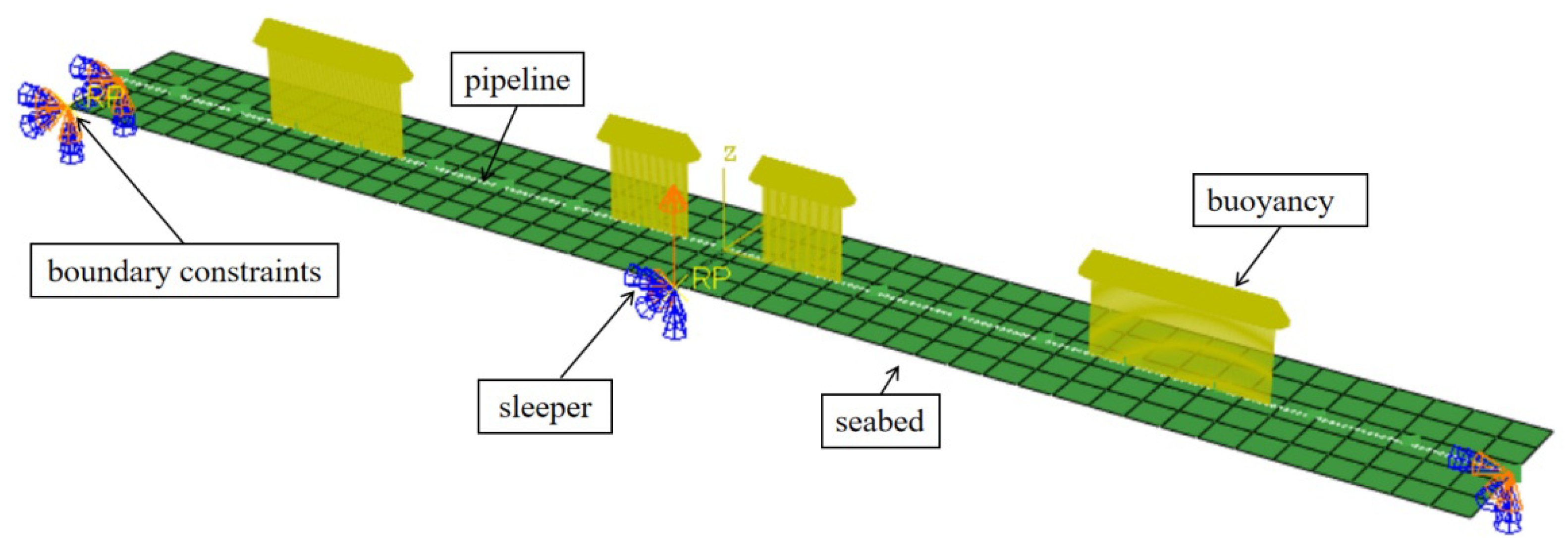
The main factors affecting the global buckling of a PIP system under the distributed buoyancy method include bending stiffness, buoyancy specific gravity, initial imperfection, pipe–sleeper friction coefficient, and stiffness ratio. Therefore, for an initial defect of a particular shape, the critical buckling axial force of the pipeline can be expressed as follows:

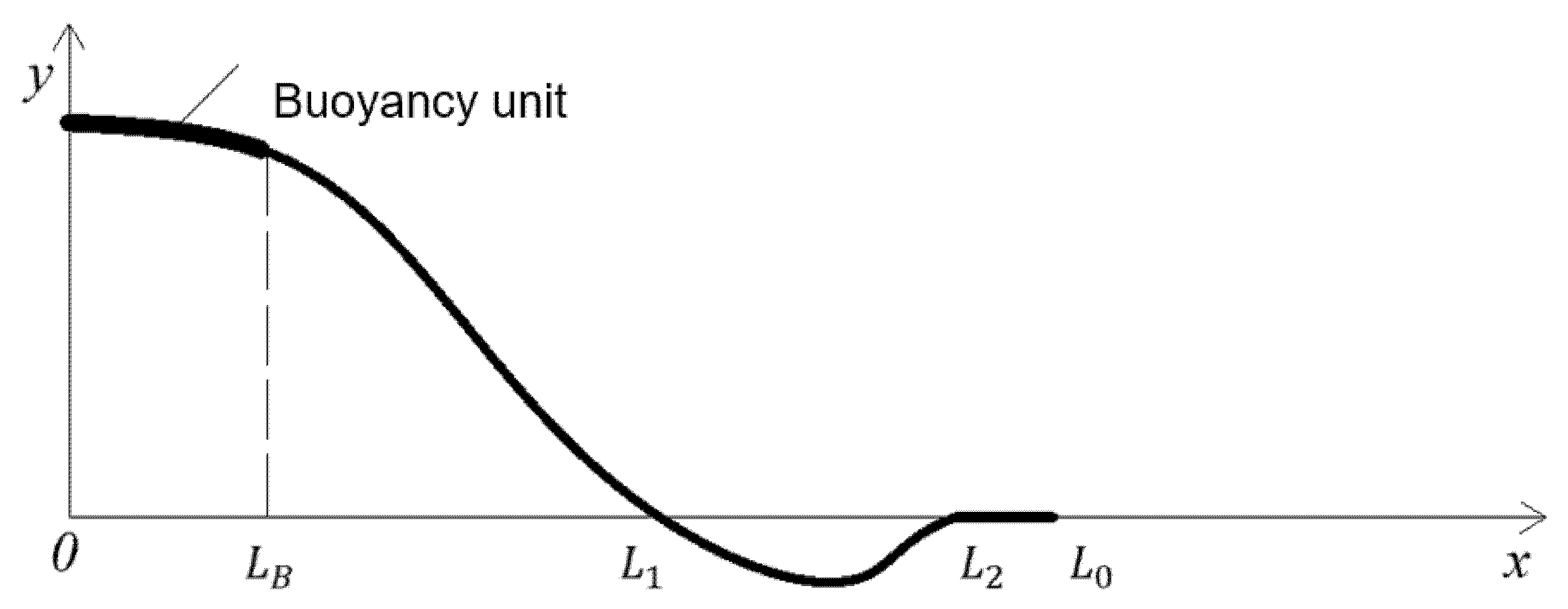
On the basis of symmetry, the lateral buckling mode of the PIP system under the distributed buoyancy method is selected and shown in Figure 11. The X-0-Y coordinate is the projection surface of the pipeline on the seabed, in which the X direction is the axial direction of the pipeline, and the Y direction is the lateral direction of the pipeline. After buckling, the pipeline can be divided into three sections according to its deformation morphology and structural characteristics. The $0\le \mathrm{x}\le {\mathrm{L}}_{\mathrm{B}}$ section is the buoyancy unit installation section, where the pipeline buoyancy is defined as ${\mathsf{\gamma }\mathrm{W}}_{\mathrm{s}}$ and the ratio of buoyancy module section length to buckling section pipeline length is $\mathsf{\beta }$, that is, $\mathsf{\beta }={\mathrm{L}}_{\mathrm{B}}/{\mathrm{L}}_1$. The pipeline displacement and strain of the buoyancy unit section are marked as “B” below. The main buckling section of the pipeline is section $0\le \mathrm{x}\le {\mathrm{L}}_1$, in which ${\mathrm{L}}_{\mathrm{B}}<\mathrm{x}\le {\mathrm{L}}_1$ does not contain a buoyancy unit. 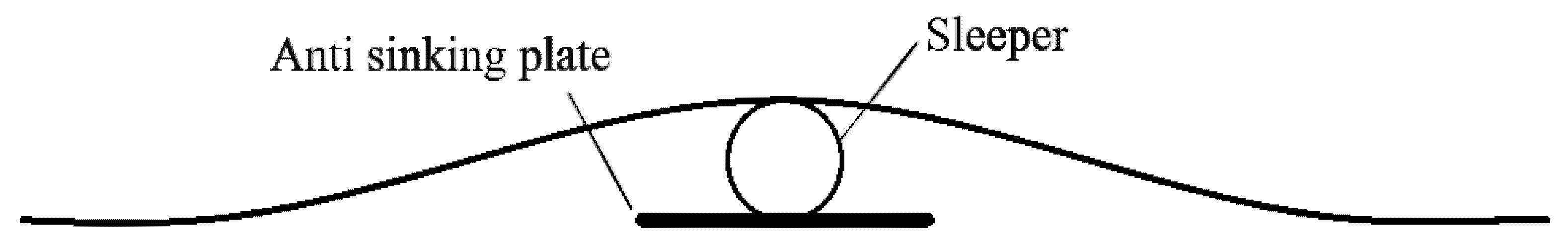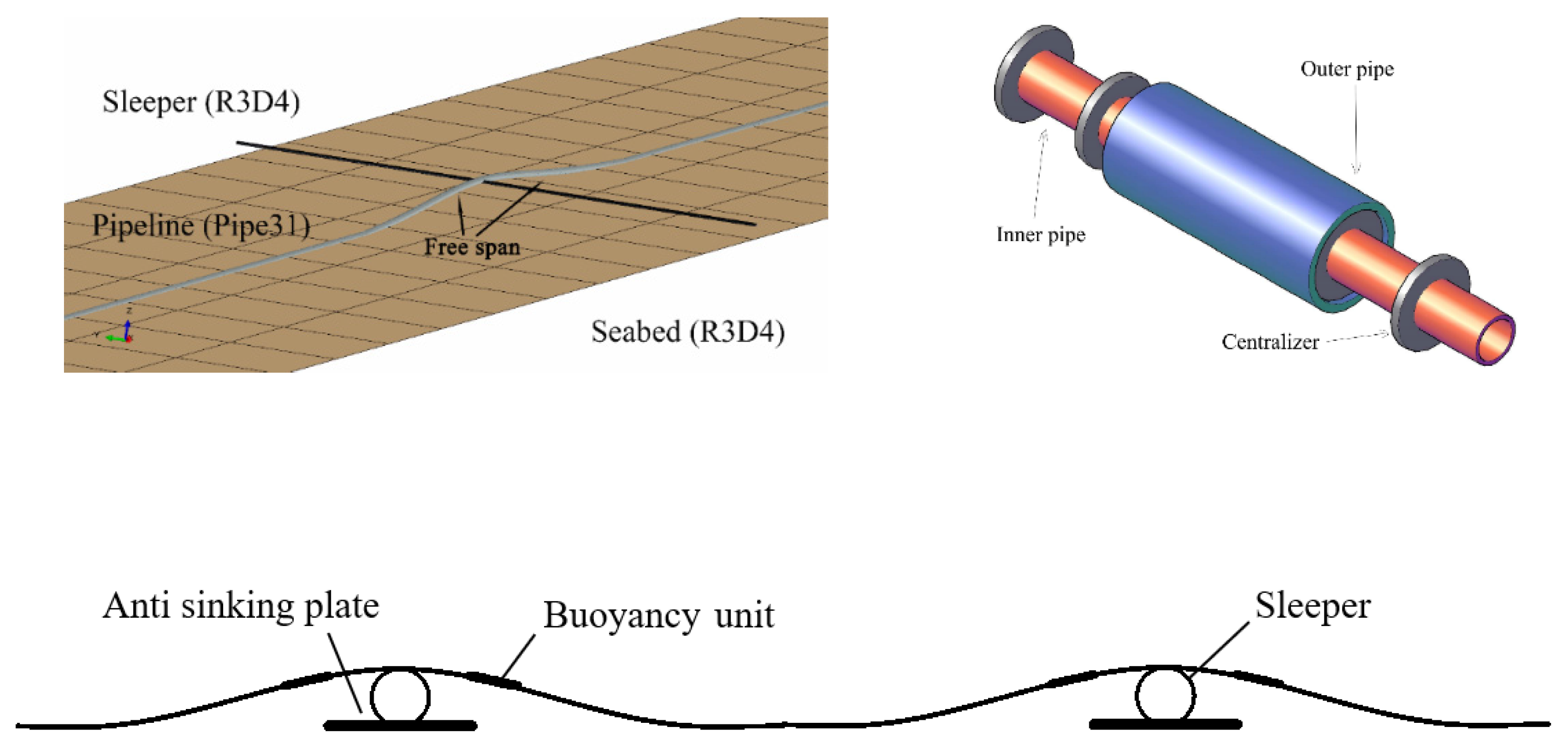The pipeline $0\le \mathrm{x}\le {\mathrm{L}}_1$ is separated from the seabed surface due to the sleeper, thereby resulting in a suspension span. The displacement and strain of the pipeline are expressed by the following standard “1.” Section ${\mathrm{L}}_{\mathrm{B}}\le \mathrm{x}\le {\mathrm{L}}_2$ is the secondary buckling section, and the displacement and strain of the pipeline are expressed as “2” below. ${\mathrm{L}}_2\le \mathrm{x}\le {\mathrm{L}}_0$ is the axial slip section, and the displacement and strain of the pipeline are marked as “3.” The virtual anchorage point is at $\mathrm{x}={\mathrm{L}}_0$, and the floating weight of pipeline in ${\mathrm{L}}_{\mathrm{B}}\le \mathrm{x}\le {\mathrm{L}}_0$ section is ${\mathrm{W}}_{\mathrm{S}}$.

According to the principle of virtual displacement, equilibrium equations can be established in different sections of the pipeline.

$$\mathrm{EI}{v}_B^{⁗}+P{v}_B^{″}=-\gamma W_s{\mu }_s$$

(2)

$$\mathrm{EI}{v}_1^{⁗}+P{v}_1^{″}=-(\gamma W_s+W_s){\mu }_s$$

(3)

$$\mathrm{EI}{v}_2^{⁗}+P{v}_2^{″}=-W_s{\mu }_L$$

(4)

$$P_0-E{A}_t{\epsilon }_B=P$$

(5)

$$P_0-E{A}_t{\epsilon }_1=P$$

(6)

$$P_0-E{A}_t{\epsilon }_2=P$$

(7)

$$\mathrm{E}{A}_t{u}_0^{″}=-{\mu }_A{W}_S$$

(8)

$${\epsilon }_i=u_i^{\prime }+\frac{1}{2}{v_i^{\prime }}^2 i=B,1, 2$$

(9)

where $v_i$ is the lateral displacement of the pipeline in the corresponding section, $u_i$ is the axial displacement of the pipeline in the corresponding section, ${\mu }_A$ is the axial friction coefficient of seabed and pipeline, ${\mu }_L$ is the lateral friction coefficient of seabed and pipeline, and ${\mu }_s$ is the friction coefficient of pipeline and sleeper. On the basis of the hypothesis of small deformation, the second derivative contribution of axial displacement is neglected. The satisfiable formula (9), $A_t=A_{in}+A_{out}$ is fulfilled.

According to the mathematical forms of Equations (2)–(4), the general solution can be obtained as a lateral displacement function that satisfies the following forms:

$$v_B\left(x\right)=A_1\cos \left(\lambda x\right)+A_2\sin \left(\lambda x\right)+A_{3}x+A_4-\frac{\gamma {\omega }_1}{2{\lambda }^2}{x}^2$$

(10)

$$v_1\left(x\right)=A_5\cos \left(\lambda x\right)+A_6\sin \left(\lambda x\right)+A_{7}x+A_8-\frac{\gamma {\omega }_2}{2{\lambda }^2}{x}^2$$

(11)

$$v_2\left(x\right)=A_9\cos \left(\lambda x\right)+A_{10}\sin \left(\lambda x\right)+A_{11}x+A_{12}-\frac{\gamma {\omega }_3}{2{\lambda }^2}{x}^2$$

(12)

where

$${\lambda }^2=\frac{P}{EI}$$

(13)

$${\omega }_3=\frac{{\mu }_L{W}_s}{EI}, {\omega }_2=\frac{(\gamma W_s+W_s){\mu }_s}{EI}, {\omega }_1=\frac{\gamma W_s{\mu }_s}{EI}.$$

(14)

Equation (8) is introduced into Equations (4)–(6) to obtain the axial and lateral displacements of buckling pipelines.

$$u_B^{\prime }\left(x\right)=\frac{\left(P_0-P\right)}{E{A}_t}-\frac{1}{2}{v_B^{\prime }}^2\left(x\right)$$

(15)

$$u_1^{\prime }\left(x\right)=\frac{\left(P_0-P\right)}{E{A}_t}-\frac{1}{2}{v_1^{\prime }}^2\left(x\right)$$

(16)

$$u_2^{\prime }\left(x\right)=\frac{\left(P_0-P\right)}{E{A}_t}-\frac{1}{2}{v_2^{\prime }}^2\left(x\right)$$

(17)

The axial displacement function of the pipeline in the slip section can be obtained by integrating Equation (7).

$$u_3\left(x\right)=-\frac{u_A{W}_s}{E{A}_t}\frac{x^2}{2}+B_{1}x+B_2$$

(18)

In the above formula, $B_1$, $B_2$, and $A_i\left(i=1\text{–}12\right)$ are undetermined displacement coefficients. The axial and lateral displacements of the pipeline should satisfy the following boundary conditions and connection conditions at the boundary of the pipeline and at the junction of each section:

Lateral displacement $v_B$ should be satisfied at $x=0$ as follows:

$$v_B^{\prime }=0,$$

(19)

$$v_B^{‴}=0.$$

(20)

Lateral displacements $v_B$ and $v_1$ satisfy the continuous boundary conditions at $x=L_B$ as follows:

$$v_B\left(L_B\right)=v_1\left(L_B\right),$$

(21)

$$v_B^{\prime }\left(L_B\right)=v_1^{\prime }\left(L_B\right),$$

(22)

$$v_B^{″}\left(L_B\right)=v_1^{″}\left(L_B\right),$$

(23)

$$v_B^{‴}\left(L_B\right)=v_1^{‴}\left(L_B\right).$$

(24)

Lateral displacements $v_1$ and $v_2$ satisfy the following continuous boundary conditions at $x=L_1$:

$$v_1\left(L_1\right)=0,$$

(25)

$$v_2\left(L_1\right)=0,$$

(26)

$$v_1^{\prime }\left(L_1\right)=v_2^{\prime }\left(L_1\right),$$

(27)

$$v_1^{″}\left(L_1\right)=v_2^{″}\left(L_1\right),$$

(28)

$$v_1^{‴}\left(L_1\right)=v_2^{‴}\left(L_1\right).$$

(29)

Lateral displacement $v_1$ satisfies the following continuous boundary conditions at $x=L_2$:

$$v_2\left(L_2\right)=0,$$

(30)

$$v_2^{\prime }\left(L_2\right)=0,$$

(31)

$$v_2^{″}\left(L_2\right)=0.$$

(32)

Axial displacement $u_B$ should satisfy at $x=0$ as follows:

$$u_B\left(0\right)=0$$

(33)

Axial displacements $u_B$ and $u_1$ satisfy continuous boundary conditions at $x=L_B$ as follows:

$$u_B\left(L_B\right)=u_1\left(L_B\right),$$

(34)

$$u_B^{\prime }\left(L_B\right)=u_1^{\prime }\left(L_B\right).$$

(35)

Axial displacements $u_1$ and $u_2$ satisfy the following continuous boundary conditions at $x=L_1$:

$$u_1\left(L_1\right)=u_2\left(L_1\right),$$

(36)

$$u_1^{\prime }\left(L_1\right)=u_2^{\prime }\left(L_1\right).$$

(37)

Axial displacements $u_2$ and $u_3$ satisfy the following continuous boundary conditions at $x=L_2$:

$$u_2\left(L_2\right)=u_3\left(L_2\right),$$

(38)

$$u_2^{\prime }\left(L_2\right)=v_3^{\prime }\left(L_2\right).$$

(39)

Axial displacement $u_3$ satisfies the following continuous boundary conditions at $x=L_0$:

$$v_3\left(L_0\right)=0,$$

(40)

$$v_3^{\prime }\left(L_0\right)=0.$$

(41)

The lateral displacement functions (10)–(12) are introduced into the lateral displacement boundary conditions (18)–(24) and (25)–(30) to obtain the undetermined coefficients of the lateral displacement function.

The lateral displacement function $v_B\left(x\right)$ coefficient of buoyancy unit in lateral displacement buckling is

$$A_1=-\frac{{\omega }_1\left\{\left[2\cos \left(\lambda L_1\right)+\left(\gamma -1\right)C\cos \left(\beta \lambda L_2\right)\right]\sin \left(\lambda L_2\right)\right\}}{{\lambda }^4\sin \left(\lambda L_2\right)}+\frac{{\omega }_1\left\{\left[2\cos \left(\lambda L_1\right)+\left(\gamma -1\right)\sin \left(\beta \lambda L_2\right)\right]\cos \left(\lambda L_2\right)-\left[\left(\gamma -1\right)\beta +2\right]\lambda L_1+\lambda L_2\right\}}{{\lambda }^4\sin \left(\lambda L_2\right)},$$

(42)

$$A_2=A_3=0,$$

(43)

$$A_4=-\frac{{\omega }_1\left\{\left[\left(\gamma -1\right)\beta \left(\beta -2\right)-1\right]{\left(\lambda L_1\right)}^2\sin \left(\lambda L_2\right)\right\}}{{\lambda }^4\sin \left(\lambda L_2\right)}+\frac{{\omega }_1\left\{\left[4\sin \left(\lambda L_2-\lambda L_1\right)\cos \left(\lambda L_1\right)-2\left(\gamma -1\right)\sin \left(\beta \lambda L_1\right)\right]\sin \left(\lambda L_1\right)\sin \left(\lambda L_2\right)\right\}}{2{\lambda }^4\sin \left(\lambda L_2\right)}+\frac{{\omega }_1\left\{2\left(\gamma -1\right)\cos \left(\beta \lambda L_1\right)\cos \left(\lambda L_2\right)\sin \left(\beta \lambda L_1\right)2\left(\gamma -1\right)\beta \lambda L_1\cos \left(\lambda L_1\right)\right\}}{2{\lambda }^4\sin \left(\lambda L_2\right)}+\frac{{\omega }_1\left\{2\left(2\lambda L_1-L_2\right)\cos \left(\lambda L_1\right)+2\left(\gamma -1\right)\sin \left(\lambda L_2\right)\right\}}{2{\lambda }^4\sin \left(\lambda L_2\right)}.$$

(44)

The displacement function $v_1\left(x\right)$ coefficient of the main buckling section without buoyancy is

$$A_5=\frac{{\omega }_2\left\{\left[2\sin \left(\lambda L_1\right)+\left(\gamma -1\right)\sin \left(\beta \lambda L_2\right)\right]\cos \left(\lambda L_2\right)\right\}}{{\lambda }^4\sin \left(\lambda L_2\right)}-\frac{{\omega }_2\left\{\left[2\cos \left(\lambda L_1\right)\sin \left(\lambda L_2\right)\right]+\left(\gamma -1\right)\beta \lambda L_1+2\lambda L_1-\lambda L_2\right\}}{{\lambda }^4\sin \left(\lambda L_2\right)},$$

(45)

$$A_6=\frac{{\omega }_2\left(\gamma -1\right)\sin \left(\beta \lambda L_1\right)}{{\lambda }^4}.$$

(46)

$$A_7=-\frac{{\omega }_2\beta L_1\left(\gamma -1\right))}{{\lambda }^4}.$$

(47)

$$A_8=-\frac{{\omega }_2\left\{\left[-2\left(\gamma -1\right)\beta -1\right]{\left(\lambda L_1\right)}^2\sin \left(\lambda L_2\right)+2\left(\gamma -1\right)\sin \left(\beta \lambda L_1\right)\cos (\lambda L_1-\lambda L_2)\right\}}{2{\lambda }^4\sin \left(\lambda L_2\right)}-\frac{{\omega }_2\left\{4\sin \left(\lambda L_2-\lambda L_1\right)\cos \left(\lambda L_1\right)-2\left[\left(\gamma -1\right)\beta \lambda L_1+2\lambda L_1-\lambda L_2\right]\left(\gamma -1\right)\cos \left(\lambda L_1\right)\right\}}{2{\lambda }^4\sin \left(\lambda L_2\right)}.$$

(48)

The lateral displacement function $v_2\left(x\right)$ coefficient of the secondary buckling section is

$$A_9=\frac{{\omega }_3\left\{\left[2\sin \left(\lambda L_1\right)+\left(\gamma -1\right)\sin \left(\beta \lambda L_2\right)\right]\cos \left(\lambda L_2\right)-\left[\left(\gamma -1\right)\beta +2\right]\lambda L_1+\lambda L_2\right\}}{{\lambda }^4\sin \left(\lambda L_2\right)},$$

(49)

$$A_{10}=\frac{{\omega }_3\left[\left(\gamma -1\right)\sin \left(\beta \lambda L_1\right)+2sin\left(\lambda L_1\right)\right]}{{\lambda }^4},$$

(50)

$$A_{11}=-\frac{{\omega }_3\left(\gamma \beta -\beta +2\right)L_1)}{{\lambda }^4},$$

(51)

$$A_{12}=\frac{{\omega }_3\left\{\left[2\left(\gamma -1\right)\beta +2\right]\lambda L_1\lambda L_2\sin \left(\lambda L_2\right)-{\left(\lambda L_2\right)}^2\sin \left(\lambda L_2\right)\right\}}{2{\lambda }^4\sin \left(\lambda L_2\right)}+\frac{{\omega }_3\left\{2\left[\left(\gamma \beta -\beta +2\right)\lambda L_1-\lambda L_2\right]\cos \left(\lambda L_2\right)-4\sin \left(\lambda L_1\right)-2\left(\gamma -1\right)\sin \left(\beta \lambda L_1\right)\right\}}{2{\lambda }^4\sin \left(\lambda L_2\right)}.$$

(52)

Lateral displacement functions (10)–(12) are introduced into boundary conditions (24) and (38) to obtain the dimensionless parameters lambda $\lambda L_1$ and lambda $\lambda L_2$, which must satisfy the following characteristic equations:

$$2\left[\left(\gamma -1\right)\cos \left(\lambda L_1-\lambda L_2\right)-\gamma +1\right]\sin \left(\beta \lambda L_1\right)+44\sin \left(\lambda L_2-\lambda L_1\right)\cos \left(\lambda L_1\right)+4\left[\sin \left(\lambda L_2\right)-\sin \left(\lambda L_1\right)\right]+2\left\{\left[\left(\gamma -1\right)\beta +2\right]\left[\cos \left(\lambda L_2\right)-\cos \left(\lambda L_1\right)\right]\right\}\left(\lambda L_1\right)-2\left[\cos \left(\lambda L_2\right)-\cos \left(\lambda L_1\right)\right]\lambda L_2-\left(2\gamma \beta -2\beta +3\right){\left(\lambda L_1\right)}^2\sin \left(\lambda L_2\right)+2\left(\gamma \beta -\beta +2\right)\lambda L_1\lambda L_2\sin \left(\lambda L_2\right)-{\left(\lambda L_2\right)}^2\sin \left(\lambda L_2\right)=0,$$

(53)

$$\left(\gamma -1\right) \sin \left(\beta \lambda L_1\right)-\sin \left(\lambda L_2\right)+2\sin \left(\lambda L_1\right)-\left[\left(\gamma \beta -\beta +2\right)\lambda L_1-\lambda L_2\right]\cos \left(\lambda L_2\right)=0.$$

(54)

Formula (15) is integrated and introduced into boundary condition (34) to obtain the axial displacement function of the buoyancy section as follows:

$$u_B\left(x\right)=\frac{\left(P_0-p\right)}{E{A}_t}x-\frac{1}{2}{{\displaystyle \int }}_0^x{v}_B^{\prime }\left(x\right)dx.$$

(55)

Formula (16) is integrated from $L_B$ to X, and boundary condition (34) is introduced to obtain the axial displacement function of the main buckling section of the pipeline without buoyancy module as follows:

$$u_1\left(x\right)=\frac{\left(P_0-P\right)}{E{A}_t}\left(x-L_B\right)-\frac{1}{2}{{\displaystyle \int }}_{L_B}^x{v}_B^{\prime }\left(x\right)dx+u_B\left(L_B\right)$$

(56)

Formula (17) is integrated from $L_1$ to X and introduced into boundary condition (37) to obtain the axial displacement function of the secondary buckling section of the pipeline as follows:

$$u_2\left(x\right)=\frac{\left(P_0-P\right)}{E{A}_t}\left(x-L_1\right)-\frac{1}{2}{{\displaystyle \int }}_{L_1}^x{v}_2^{\prime }\left(x\right)dx+u_1\left(L_1\right).$$

(57)

The expressions of the axial displacement function can be obtained by introducing the slip section axial displacement function (18) into boundary conditions (40), (41) as follows:

$$u_3\left(x\right)=\left[\frac{{\mu }_A{W}_S}{2E{A}_t}\left(x+L_0-2L_2\right)-\frac{\left(P_0-P\right)}{EA}\right]\left(L_0-x\right).$$

(58)

The relationship between the axial load of the buckling section of the pipeline and the axial load of the virtual anchorage point can be obtained by introducing the upper formula to the boundary condition (41) as follows:

$$P-P_0={\mu }_A{W}_S\left(L_0-L_1\right).$$

(59)

The lateral buckling equation can then be obtained as

$$P_0=P+{\mu }_A{W}_S{L}_2\left[-1+\sqrt{1+\frac{E{A}_t}{{\mu }_A{W}_S{L}_2^2}\left({{\displaystyle \int }}_{L_B}^x{v_B^{\prime }}^2\left(x\right)dx+{{\displaystyle \int }}_{L_1}^x{v_2^{\prime }}^2\left(x\right)dx+{{\displaystyle \int }}_0^x{v_B^{\prime }}^2\left(x\right)\right)}\right],$$

(60)

$$P={\left(\frac{\lambda L_i}{L}\right)}^2\mathrm{EI},$$

(61)

where $\mathrm{EI}={\mathrm{E}}_1{\mathrm{I}}_1+{\mathrm{E}}_2{\mathrm{I}}_2$.

4.2. Formula Validation

The following parameters of the PIP system are selected to verify the accuracy of the formulas, as shown in

Table 9. Parameters of the PIP system.

Parameter of the PIP System	Value
Inner pipe diameter (mm)	40
Outer pipe diameter (mm)	46
Inner pipe wall thickness (mm)	5
Outer pipe wall thickness (mm)	5
Modulus of elasticity (Gpa)	207
Poisson ratio	0.3
Pipe floating weight (KN/m)	3300
Design temperature (°C)	50
Coefficient of thermal expansion (1/°C)	1.17 × 10−5
Axial friction coefficient	0.5
Lateral friction coefficient	0.5

.

A comparison of the FE model result and analytic solutions in

Table 10. Comparison of the results.

	Buckling Length	Axial Force in Buckling Segment	Maximum Lateral Displacement
FE model	110.5	9.53 × 103	6.87
Analytic solutions	114.8	9.68 × 103	6.92
Error%	3.8	1.5	0.7

shows that the error of the analytic solutions is consistent with that of the FE model, indicating that the formulas have high accuracy in forecasting the global buckling of the PIP system.

5. Conclusions

In this study, a FE model for the active control buckling of PIP systems under the SDB method is established, and the effects of different parameters on the global buckling are analyzed. The accuracy of the model is verified by existing projects. On the basis of the analysis results for the FE model, the formulas for calculating the critical buckling axial force and lateral displacement of this type of pipeline are obtained by analytical solution. The main conclusions are as follows:

• The proposed SDB method to control the global buckling of PIP systems can solve the instability caused by the high center of gravity of the pipeline under the sleeper control method and the extremely large outer diameter of pipelines wrapped by buoyancy unit under the buoyancy method.
• Geometric model and FE models of PIP systems under combined control by the SDB method are proposed, and the accuracy of the models is verified. Parametric analysis shows that the bending stiffness, buoyancy ratio, initial defects, and stiffness ratio of inner and outer pipes are the main factors affecting the critical buckling force of pipelines.
• The critical buckling axial force and lateral displacement formulas of pipelines are deduced and validated by analytical solution. A comparison shows that the formulas have high accuracy and can meet the requirements for engineering design.

References

1. Wang, Z.; Chen, Z.; Liu, H. On lateral buckling of subsea pipe-in-pipe systems. Int. J. Steel Struct. 2015, 15, 881–892. [Google Scholar] [CrossRef]
2. Liu, R.; Li, C. Determinate dimension of numerical simulation model in submarine pipeline global buckling analysis. Ocean Eng. 2018, 152, 26–35. [Google Scholar] [CrossRef]
3. Zeng, X.G.; Duan, M.L.; Che, X.Y. Analysis on upheaval buckling of buried subsea PIP pipeline. The Ocean Eng. 2014, 32, 72–77. [Google Scholar]
4. Zeng, X.; Duan, M.; Che, X. Critical upheaval buckling forces of imperfect pipelines. Appl. Ocean. Res. 2014, 45, 33–39. [Google Scholar] [CrossRef]
5. Wang, Z.; Chen, Z.; Liu, H. Numerical study on upheaval buckling of pipe-in-pipe systems with full contact imperfections. Eng. Struct. 2015, 99, 264–271. [Google Scholar] [CrossRef]
6. Liu, R.; Hao, X.; Wu, X.; Yan, S. Numerical studies on global buckling of subsea pipelines. Ocean Eng. 2014, 78, 62–72. [Google Scholar] [CrossRef]
7. Karampour, H.; Albermani, F.; Gross, J. On lateral and upheaval buckling of subsea pipelines. Eng. Struct. 2013, 52, 317–330. [Google Scholar] [CrossRef]
8. Zhang, Z.; Liu, H.; Chen, Z. Lateral Buckling Theory and Experimental Study on Pipe-in-Pipe Structure. Metals 2019, 9, 185. [Google Scholar] [CrossRef] [Green Version]
9. Wang, Z.; Tang, Y.; Feng, H.; Zhao, Z.; Liu, H. Model Test for Lateral Soil Resistance of Partially Embedded Subsea Pipelines on Sand during Large-Amplitude Lateral Movement. J. Coast. Res. 2017, 33, 607–618. [Google Scholar]
10. Zechao, Z.; Zhihua, C.; Hongbo, L.; Zhe, W.; Kaiyue, L. Study of Dynamic Effect on Lateral Buckling of Pipe-in-Pipe System with Initial Imperfections. J. Tianjin Univ. 2019, 52, 404–412. [Google Scholar]
11. Reddy, N.R. Lateral Buckling Behaviour of Snake-Lay Pipeline with Vertical Support at Crown. In International Conference on Offshore Mechanics and Arctic Engineering; American Society of Mechanical Engineers: New York, NY, USA, 2013; Volume 55362, p. V04AT04A010. [Google Scholar]
12. Proc, K.; Chaney, L. Thermal Load Reduction of Truck Tractor Sleeper Cabins. Sae Int. J. Commer. Veh. 2008, 1, 268–274. [Google Scholar] [CrossRef]
13. Sun, J.; Paul, J.; Han, S. Thermal Expansion/Global Buckling Mitigation of HPHT Deep-Water Pipelines, Sleeper or Buoyancy. In Proceedings of the 22nd International Offshore and Polar Engineering Conference, Rhodes, Greece, 17–22 June 2012. [Google Scholar]
14. Rundsag, J.O.; Tørnes, K.; Cumming, G.; Rathbone, A.D.; Roberts, C. Optimised Snaked Lay. In Proceedings of the Eighteenth International Offshore and Polar Engineering Conference, Vancouver, BC, Canada, 6–11 July 2008. [Google Scholar]
15. Che, X.Y.; Duan, M.L.; Zeng, X.G.; Gao, P.; Pang, Y.Q. Experimental Study and Numerical Simulation of Global Buckling of Pipe-in-Pipe Systems. Appl. Math. Mech. 2014, 35, 188–201. [Google Scholar]
16. Alrsai, M.; Karampour, H.; Albermani, F. Numerical study and parametric analysis of the propagation buckling behaviour of subsea pipe-in-pipe systems. Thin Walled Struct. 2018, 125, 119–128. [Google Scholar] [CrossRef] [Green Version]
17. Westgate, Z.J.; Randolph, M.F.; White, D.J.; Brunning, P. Theoretical, numerical and field studies of offshore pipeline sleeper crossings. In Proceedings of the 2nd International Symposium on Frontiers in Offshore Geotechnics, Perth, Australia, 7–12 November 2011; pp. 845–850. [Google Scholar]
18. Peek, R.; Yun, H. Flotation to trigger lateral buckles in pipelines on a flat seabed. J. Eng. Mech. 2007, 133, 442–451. [Google Scholar] [CrossRef]
19. Gang, L. Multi-Objective Optimization Design for Lateral Buckling Control of Subsea Pipelines by Distributed Buoyancy Sections. Appl. Math. Mech. 2016, 9, 945–955. [Google Scholar]
20. Denniel, S.; Ross, R.A.L. Method and Apparatus for Mounting Distributed Buoyancy Modules on a Rigid Pipeline. U.S. Patent 8,573,888, 5 November 2013. [Google Scholar]
21. Cumming, G.; Rathbone, A. Euler Buckling of Idealised Horizontal Pipeline Imperfections. In International Conference on Offshore Mechanics and Arctic Engineering; American Society of Mechanical Engineers: New York, NY, USA, 2010; Volume 49132, pp. 293–300. [Google Scholar]
Figure 1. Sketch map of the sleeper method.
Metals 12 01094 g001
Figure 2. Sketch map of the SDB method.
Metals 12 01094 g002
Figure 3. FE model of SDB.
Metals 12 01094 g003
Figure 4. Result of a PIP system on global buckling. (a) Displacement development; (b) stress development.
Metals 12 01094 g004
Figure 5. Influence of the buoyancy density in the axial force–lateral displacement graph.
Metals 12 01094 g005
Figure 6. Influence of the pipe–soil friction coefficient in the axial force–lateral displacement graph.
Metals 12 01094 g006
Figure 7. Influence of initial imperfection in the axial force–lateral displacement graph.
Metals 12 01094 g007
Figure 8. Influence of the rigidity ratio of inner and outer pipes in the axial force–lateral displacement graph.
Metals 12 01094 g008
Figure 9. Influence of sleeper height in the axial force–lateral displacement graph.
Metals 12 01094 g009
Figure 10. Influence of buoyancy unit interval in the axial force–lateral displacement graph.
Metals 12 01094 g010
Figure 11. Force diagram of SDB.
Metals 12 01094 g011