Article

Study of Quenched Crankshaft High-Cycle Bending Fatigue Based on a Local Sub Model and the Theory of Multi-Axial Fatigue

College of Automobile and Traffic Engineering, Nanjing Forestry University, Nanjing 210037, China
*
Author to whom correspondence should be addressed.
Metals 2022, 12(6), 913; https://doi.org/10.3390/met12060913
Submission received: 11 April 2022 / Revised: 21 May 2022 / Accepted: 23 May 2022 / Published: 26 May 2022

Abstract

:
For critical steel engine parts, such as crankshafts, the fatigue strength under the critical working condition is usually improved by the electromagnetic induction quenching technique. In a previous study, the strengthening effect of this approach was always evaluated by a constant, which may result in some errors with the change of the technological parameters. In this paper, a type of steel crankshaft is selected to study the strengthening effect of this approach; first a local sub model composed of the crankpin is built to simulate the magnetic–thermal coupling process, then, the residual stress field is determined by simulating the whole course of fabrication. Finally, the prediction of the fatigue limit load is proposed based on the residual stress and the strength parameters of the material. The experimental verification shows that, when compared to the general means of modification models, the modified McDiarmid multi-axial fatigue model is more suitable to be applied to analyze the fatigue property of this quenched crankshaft due to the markedly higher accuracy. Based on this study, a new fatigue-limit load-prediction approach of this kind of crankshaft can be proposed for engineering applications.

1. Introduction

Nowadays, family cars are widely used in daily life. For this modern mechanical equipment, various dynamic loads are applied to the parts [1,2]. Thus, a special surface strengthening method is necessary to ensure that the parts can fulfil the corresponding service life requirements. Among these methods, the electromagnetic induction quenching approach is considered to be an effective choice [3,4]. This technique can effectively improve the fatigue strength of the metal parts, such as the steel crankshafts, to make them applicable to the high-power engine, thus corresponding technique parameters are necessary to be reasonably planned during the design stage.
In recent years, some experts focused on researching this problem. Among them, Cajner proposed a 2D simplified axial symmetrical model to conduct the numerical simulation of the electromagnetic induction quenching approach on a 42CrMo steel crankshaft; the experimental verification showed that this model can provide accurate surface hardness and hardness layer-depth results [5]. Dmitry conducted a technological parameter influence analysis of this approach and proposed a corresponding model to accurately simulate the process [6]. Mohan proposed a new optimal design method based on a satisfactory function, which was established during the electromagnetic induction quenching process [7]. Stephanie compared the mechanical and microstructure properties of the 42CrMo steel after electromagnetic induction quenching and conventional heat treatment process through the standard tensile experiment and pyramid hardness test. The result showed that yield strength and hardness of the steel after electromagnetic induction quenching were a little lower than those of the steel after a conventional heat treatment process, which can be attributed to the size effect [8]. Dietmar applied the adaptive finite element analysis approach in simulating the electromagnetic induction quenching of the gear and obtained accuracy for the temperature and hardening curve [9]. Umberto researched the microstructure and mechanical property of the hardening layer and proposed that the main influence factors were the heating and cooling speeds during the electromagnetic induction quenching, as well as the peak value of the temperature [10]. Akram proposed novel alternate magnetic field treatments in EN8 steel and discovered that this approach could improve the wear resistance and reduce the coefficient of the friction of the material, which could be explained by the increase in the compressive residual stress and the microhardness. This method can also be applied to the fatigue property research of similar metal materials [11].
Nowadays, the turbocharging technique has been widely applied for improving the engine power, which results in the more critical demand for the fatigue strength of some key metal parts, such as the crankshaft. As a result of this, a more accurate assessment of the strengthening effect of this approach is necessary. However, the strengthening effect of this approach has not been quantitatively evaluated. In addition, the heat-up process of the electromagnetic induction quenching approach is usually no more than 20 s and corresponding components are surrounded by the coil. This situation makes the real-time experiment verification difficult to conduct.
In a previous study, we evaluated the strengthening effect of this technique by considering the residual stress as the mean stress and applied corresponding mean stress models to the prediction of the fatigue limit load of a given type of steel crankshaft [12,13]. The theoretical foundation of this approach is that both the mean and alternating stresses are uniaxial and in the same direction; whereas, for the parts with complicated shapes, the state of the alternating stress is usually multi-axial, even though the load applied to it is the uniaxial type [14,15]. This situation makes the application of the mean stress models unreasonable to some degree.
In this paper, a comprehensive assessment of the strengthening effect of the electromagnetic induction quenching technique is conducted. First, the whole process of this approach is simulated by a finite element model to provide the basic stress and temperature information. Then, a combination of the residual stress field obtained in a previous chapter and a verified multi-axial fatigue model are chosen to predict the fatigue limit load of the crankshaft. Finally, the predictions based on different models are checked by the corresponding experiment verification. The results show that, when compared to the usual modified models based on the mean stress, the modified McDiarmid multi-axial fatigue model can exhibit higher accuracy in this prediction, thus possessing practicability and value of popularization in actual engineering applications.

2. Materials and Methods

2.1. The Prediction Process

Figure 1 shows the structural property of the electromagnetic induction quenching equipment, from which it can be determined that the whole equipment can be divided into three parts: the crankpin coil, the fillet coil, and the magnetizer between the coils and the crankshaft.
According to the fatigue damage theory, the quenching process used in actual engineering applications is considered for improving the fatigue strength of a given part in two ways: changing the structural stress and generating the compressive residual stress at the stress concentration point. During the quenching process, the same electric current flows through the coil during the quenching process. Due to the smaller cross-sectional area, the current density in the fillet coil is greater than that in the crankpin coil. In addition, the fillet coil is fabricated into an arc shape to ensure that the air gap between the coil and the crankshaft remains steady. In this way, a good heating effect is achieved. On the other hand, the structural stress on the crankshaft caused by the uneven material property is not obvious [12]. Based on this assumption, the prediction of the fatigue limit load of the quenched steel crankshaft can be achieved as follows:
Step 1: In this step, the whole quenching process (including the heating and cooling stages) of a given type of crankshaft (the material is high-strength alloy steel) was exhibited by the finite element analysis. In this way, the temperature field evolution process was performed in detail.
Step 2: The temperature field evolution process obtained in the previous step was chosen to be the temperature load to simulate the residual stress field after the cooling stage.
Step 3: In this step, a verified multi-axial fatigue model was selected to be applied in predicting the fatigue limit load of the treated crankshaft based on two parameters: the combination of this stress field and the residual stress field above, and the shear fatigue strength of the material. The relationship between the prediction and existing parameters can be expressed as:
τ r + M e M A τ A = τ b
In this equation, Me and MA are the prediction of the fatigue limit load and the certain load applied to the crankshaft, respectively; τ r and τ A are the effective stress of the residual stress field; and the effective stress under load MA, respectively, τ b is the shear fatigue limit of the material.

2.2. The Coordinate Transform Method

According to the prediction equation above, it is not difficult to find out that the key parameters among the prediction process are the effective stress of the residual stress field and the effective stress under the alternating load. Nowadays, these parameters are calculated based on the given stress state and the chosen multi-axial fatigue damage model. On the other hand, the critical plane approach is considered to be an effective method in researching the multi-axial fatigue components. For the simple construction objects, such as the smooth and notched specimens, the direction of the critical plane and corresponding effective stress can be easily determined by theoretical analysis; whereas, for the parts with complicated shape, such as the crankshafts, the direction of the critical plane cannot be directly determined due to the complex stress state.
In a previous study, we found that the modified McDiarmid model could provide a high enough accuracy to predict the fatigue limit load of the steel crankshaft. The critical plane according to this model is the plane with the maximum shear stress. In addition, the direction of this plane can be determined by a coordinate transform method. The principle of this method is shown in Figure 2.
As shown in Figure 2, point O is a random point in the three-dimensional space, as well as the original point of the coordinate system O-XYZ. The plane Δ is a random plane in the space that crosses point O, and n is the normal vector of this plane. The angles between the projection of the normal vector n in the coordinate system O-XYZ and the X, Z axis are θ and φ , respectively. For point O, the 3D stress tensor in the coordinate O-XYZ is expressed as:
σ = σ 11 σ 12 σ 13 σ 21 σ 22 σ 23 σ 31 σ 32 σ 33
As shown in Figure 2, the coordinate O-abn is another coordinate that also crosses point O. Therefore, the expressions of the normal vector n and the a, b axis in the coordinate system can be expressed as:
n = n x n y n z = s i n θ c o s φ s i n θ s i n φ c o s θ
a = a x a y a z = s i n φ c o s φ 0
b = b x b y b z = c o s φ c o s θ c o s θ s i n φ s i n θ
In plane Δ , m is a random line that crosses point O. The angle between this line and the axial a is α . Therefore, the expression of the unit vector along the line m is:
m = m x m y m z = c o s α s i n φ + s i n α c o s θ c o s φ c o s α c o s φ + s i n α c o s θ s i n φ s i n θ s i n α
Based on these parameters, the shear stress in the plane nom can be expressed as:
τ n s = m x m y m z T σ 11 σ 12 σ 13 σ 21 σ 22 σ 23 σ 31 σ 32 σ 33 n x n y n z
Nowadays, the stress tensor of point O in Equation (2) can be easily determined by a finite element analysis. Therefore, the shear stress in any plane that crosses the same point can be determined by changing the values of the corresponding three angles from Equations (3)–(7). In this way, the maximum value of the shear stress and corresponding critical plane direction can be determined.

3. Results

3.1. Heating Stage Analysis

3.1.1. Mesh Model and Material Parameter

In this paper, the research was conducted on a steel crankshaft from a six-cylinder diesel engine. In addition, the electromagnetic field showed obvious dissipation properties in the air [16]. As a result of this, the far field technique was chosen to build the finite element model as follows:
As shown in Figure 3, this finite element model was built based on the finite element software Altair flux. In order to reduce the simulation content, the model was only composed of a quarter of the crankpin and located in an approximately infinite field. This sub model was cut from the crankpin of the crankshaft. The distance between the coil and the crankshaft was 0.8 mm. According to the electromagnetism theory, the induced current was mainly located on the surface of the steel part. As a result of this, the temperature increased much more rapidly in this area due to the skin effect. Therefore, in this model, the mesh sizes of the surface elements were relatively smaller to provide higher accuracy; whereas, for the inner scope, the sizes of the elements were much larger to provide higher efficiency. In this way, an overall balance between the speed and accuracy could be achieved.
In this paper, the crankshaft was made of 42CrMo steel. Table 1 shows the detailed information of this material, from which it can be discovered that some of the material properties, such as the heat conductivity, change with the temperature [17].

3.1.2. Definition of the Boundary Condition

In the heating stage, the temperature field was caused by a high-frequency current, which can be considered to be the load at this stage. As shown in Table 2, a clear conclusion can be discovered that the value of the current density in either coil is different from that in the other coil, while the values of the current intensity in both coils are the same. This phenomenon can be explained by the different cross-section areas of the two coils. In addition, the working mode of the fillet was continuously heated; whereas, for the crankpin, the current was terminated for 1 s after every 0.5 s of heating.
During the heating process, the crankshaft and the coils were just placed in the air. According to the theory of thermodynamics, the thermal transmission types in this condition are heat convection and radiation. The corresponding boundary condition can, at this stage, be defined as:
λ T n = h ( T S T f )
For the parameters in the above formula, λ is the thermal conductivity, T S is the temperature of the crankshaft surface, and T f is the temperature of the air; h is the equivalent heat transfer coefficient. The corresponding transfer coefficients are 100 W/(m2·°C) and 0.8. In addition, the symmetric cross section of the model was set to be adiabatic due to the architectural feature of the crankpin.

3.1.3. Simulation Results and Analysis

From Figure 4, Figure 5, Figure 6 and Figure 7, the evolution process of the temperature field in different time nodes during the whole quenching process based on the finite element model built in the previous chapter is shown. As shown in Figure 4, the surface temperature of the fillet increases the fastest. This can be explained by the larger current density within the corresponding coil and longer heating time. After 6 s, an obvious increase can be discovered in the surface temperature of the fillet, as well as that of the crankpin. During this time node, the surface temperature was already high enough for the surface material to be transformed to austenite. However, the depth was still very thin (no more than 0.5 mm). On the other hand, the heating penetration of the fillet was obviously deeper than that of the crankpin. The reason for this phenomenon was also the differences between the working parameters. In Figure 5 and Figure 6, the range of the high-temperature field obviously extends. The values of the heating depth at the fillet and the crankpin were nearly the same. The reason for this is the heat capacity at the fillet and heat conduction under the surface. This situation is beneficial for the generation of the surface layer. In Figure 7, after 12 s, the highest temperature point reached 1099 °C. The location of this point was at the central part of the crankpin.

3.2. Cooling Process Analysis

3.2.1. Temperature Field Analysis

During this stage, the coolant was sprayed onto the surface of the crankshaft. The whole process lasted 10 s. As a result of this, an obvious decline in the surface temperature was discovered. In addition, the convective heat transfer coefficient between the crankshaft and the cooling liquid was much higher than that in the previous chapter. The detailed boundary condition information is shown in Table 3.
Figure 8, Figure 9, Figure 10 and Figure 11 show the temperature field evolution process of the crankshaft during the liquid cooling stage. The most notable feature was that, during this stage, the maximum temperature point gradually moved from the surface to the inner parts of the crankshaft. In Figure 9, the maximum temperature was 249 °C after 4 s. In Figure 10, the maximum temperature was 152 °C after 7 s. After 10 s, the surface temperature was nearly the same as the room temperature. In addition, compared to the crankpin, the cooling depth of the fillet was much higher. The main reason of this phenomenon can also be attributed to the higher heat capacity and quicker cooling speed of the former. Following this liquid cooling stage, the highest temperature dropped to 131 °C.

3.2.2. The Residual Stress Field Analysis

During this stage, the crankshaft was placed in the air until completely cooled. As a result of this, the internal thermal stress generated corresponding residual stress. In other words, the thermal load within this stage was the temperature field evolution process. Figure 12 shows the boundary condition of the finite element model during this stage. It can be concluded that the symmetrical freedom of the nodes on the symmetrical cut planes was fixed. The whole model was built based on the finite element software Abaqus.
Figure 13 shows the residual stress field of the crankshaft. It can be observed that the type of the surface stress was compressive; whereas, for the inner area, the type was converted to tensile. The maximum stress point was located at the connecting area between the fillet and the crankpin with the value of −421.2 MPa.

3.3. Prediction and Experimental Verification

3.3.1. Multi-Axial Fatigue Model Selection

According to our previous study [17], for the parts with complicated shapes, the state of the alternating stress was usually multi-axial, even though the load applied to it was the uniaxial type. As a result, the fatigue type of this part was multi-axial [14,15]. According to our previous study, the stress ratio modified McDiarmid model can provide a high enough accuracy for the bending fatigue limit load prediction of the steel crankshaft. The definition of this model can be expressed as [18]:
τ n s + ( 1 R ) τ 1 2 σ b σ n max = τ f ( 2 N f ) c
where τ n s is the shear stress amplitude on the critical plane, σ n max is the maximum value of the normal, R is the stress ratio, N f is the fatigue life, τ 1 is the shear fatigue limit of the material, σ b is the tensile strength of the material, τ f and c are both material constants. The definition of the critical plane according to this model is the plane with the maximum shear stress, which can be determined by a combined coordinate transform and finite element method. The process of this method can be divided into two steps:
  • Determine the location of the maximum stress point of the crankshaft by a finite element model and record the stress tensor of the point.
  • Calculate the values of the shear stress in every plane. In this way, the coordinate of the maximum shear stress critical plane can be determined, as well as the normal stress.

3.3.2. Prediction Based on the Multi-Axial Fatigue Model

According to the method above, the first step was to determine the maximum stress point by the finite element method. Figure 14 shows the finite element model of the analysis, from which it can be observed that the boundary condition can be treated as restricting all the freedoms of the nodes at the right face for simplification. In this paper, a determined given bending moment (1000 N·m) was applied to the crankshaft; the result is shown in Figure 15.
As shown in Figure 15, the maximum Von Mises point under this given load is located at the fillet of the crankpin, and the corresponding value is 210.8 MPa; whereas, according to Figure 13, for the residual stress field, the value of the stress at the same point is 282 MPa. Table 4 shows the main parameters of the stress tensor of this point under the given load and from the residual stress field. Based on this parameter and the coordinate transform method mentioned in the Materials and Methods Section, the normal vector of the critical plane can be determined; the corresponding values are 136°, 90°, 91°, respectively. With the help of these three parameters, the shear and normal stresses of the critical plane from different sources can be determined; the results are shown in Table 5.
Based on these parameters and the modified McDiarmid model, the fatigue limit load of the crankshaft can be predicted. According to the previous study, the stress ratio of the bending fatigue experiment was −1, so the expression of the prediction can be proposed as:
M e 1000 × 119.2 M P a 24.4 M P a + [ M e 1000 × ( 118.6 M P a ) 157.3 M P a ] × ( 1 R ) × 226 M P a 874 M P a × 2 = 226 M P a
By solving this function, the value of the fatigue limit load of this crankshaft can be determined to be 3299 N·m.

3.3.3. Other Prediction Methods and Application

In the previous study [19], some researchers proposed different mean stress models to predict the fatigue limit load. The expressions of these commonly used mean stress models are shown in Table 6.
In these equations, σ e q is the effective stress amplitude, σ a is the stress amplitude, σ 1 is the fatigue limit, σ y is the yield strength, σ m is mean stress, and σ b is the tensile strength [19]. The predictions based on these four models are shown in Table 7.

3.3.4. Experimental Verification

In order to make a comprehensive contrast of the models mentioned above, a corresponding experimental verification was conducted at this stage to check the application of the prediction approach. Figure 16 shows the bending fatigue test bench of the crankshaft that consists of the electromagnetic vibration exciter, the master arm, the slave arm, the acceleration transducer, and the foundation bed. The crankshaft and the connected arms were vertically supported by springs, and the excitation force was generated by rotating the eccentric with the motor. In this way, a cyclic bending moment was applied to the crankshaft for fatigue testing. During the experiment process, the crack was expected to appear at the fillet of the crankshaft and the stiffness of the system decreased. As a result, the responsive acceleration and the amplitude of the load may increase if the frequency of the exciter remains unchanged. To avoid this unwanted situation, the rotation speed of the exciter decreases accordingly. When the speed decreases to a certain level, the crankshaft is considered broken [15]. In this paper, the value of the decrement of the rotate speed was 60 rpm. The serial number of the experiment standard used in this paper is QC-T637-2000 [20,21]. In this paper, 10 groups of experiments were conducted. The results are shown in Figure 17.
As shown in Figure 17, the approximate liner regression relationship can be discovered between the fatigue life and the fatigue load in the double logarithmic coordinates. In addition, the squared value of the coefficient of association was 0.5265. In this paper, the sample size of the experiment was 10. According to the significance requirement of this parameter, the minimum value under this condition should be 0.497 when the significant degree is 1%. Therefore, these experimental results can be taken into the further analysis. Nowadays, most engineering equipment is required to be able to work normally during the designed working period [22,23]. In addition, the service life of a crankshaft is limited to a certain number of cycles, depending on the demand of the traveling distance. As a result, compared to the common fatigue property evaluation parameter (usually the fatigue life under a given load) [24,25], it is more important to correctly evaluate the high-cycle fatigue load of a crankshaft under a specified fatigue life [26,27]. According to the previous study, the SAFL (Statistical Analysis for Fatigue Limit) approach was considered to be an effective method to analyze the distribution property of the fatigue limit load [28]. Based on this method, the fatigue limit load prediction can be proposed. The results are shown in Table 8.

3.3.5. Prediction Errors and Discussion

According to the SAFL method, the distribution property of the fatigue limit load can be expressed by a Gaussian distribution function. As a result, the fatigue limit load of this crankshaft under a 50% survival rate was 3335 N·m.
As shown in Table 9, it can be found that the predictions based on the commonly used mean stress models results in obvious errors (the errors are all higher than 20%), which makes them inapplicable in this occasion; whereas the prediction provided by the modified McDiarmid multi-axial fatigue model is consistent with the experimental results (the error between them is less than 5%). The main reasons for this phenomenon may be analyzed by two sides:
(1)
As shown in Table 5, the types of the normal and shear stress in the critical plane caused by the residual stress field are both compressive; whereas, for the alternating stress caused by the load, the type of shear stress in this critical plane is tensile and the type of normal stress is compressive. In addition, the ratios of the shear stress and the tensile stress from different sources are not the same. As a result, the effective stresses from these two sources are not in the same direction, which is not suitable for the application of the mean stress models.
(2)
According to our previous study, the fatigue damage type of the crankshaft in this condition is shear fatigue damage, while the modified McDiarmid multi-axial fatigue model is just considered to be a typical effective model in researching this type of problem. This makes the application of this model more effective.

4. Conclusions and Further Work Plan

In this paper, a new fatigue property prediction approach of quenched metal crankshaft was proposed. First, a local sub-model composed of the crankpin was built to simulate the magnetic–thermal coupling process. Then, the residual stress field was conducted by the subsequent thermal–mechanical coupling analysis. Finally, the fatigue limit load prediction of the treated crankshaft was achieved based on the parameters obtained above and the material property. The results show that this manufacturing procedure can generate uniform temperature fields at the surface of the crankpin area during the heating-up stage, which is beneficial to the forming of the uniform layer. In addition, when compared to the commonly used mean stress models, the modified McDiarmid multi-axial fatigue model can provide a high enough accuracy in predicting the fatigue limit load of the quenched crankshaft, which makes this model valuable in guiding the design of the manufacturing procedure.
During our study, we discovered that the extraction range of the sub model would not obviously influence the temperature field; whereas, for the residual stress field, different situations were discovered. Therefore, in our further work, we will focus on the influence of this factor. In addition, the material of the crankshaft in this paper was 42CrMo. The research on the application of this model in researching the crankshafts made by some other steel materials is still needed.

Author Contributions

Conceptualization: S.S.; methodology: S.S.; software: X.Z.; validation: S.S., X.Z.; formal analysis: S.S.; investigation: S.S., X.Z.; resources: S.S.; data curation: S.S.; writing—original draft preparation: S.S.; writing—review and editing: X.G., M.W.; visualization: None; supervision: X.X.; funding acquisition: X.X. All authors have read and agreed to the published version of the manuscript.

Funding

This research received no external funding.

Institutional Review Board Statement

Not applicable.

Informed Consent Statement

Not applicable.

Data Availability Statement

All data generated or analyzed during this study are included in this published article.

Conflicts of Interest

The authors declare no conflict of interest.

References

  1. Jie, T.; Tong, J.; Shi, L. Differential steering control of four-wheel independent-drive electric vehicles. Energies 2018, 11, 2892. [Google Scholar]
  2. Tian, J.; Wang, Q.; Ding, J.; Wang, Y.; Ma, Z. Integrated Control with DYC and DSS for 4WID Electric Vehicles. IEEE Access 2019, 7, 124077–124086. [Google Scholar] [CrossRef]
  3. Zhu, Y.; Luo, Y.; Ma, N. Relationship between equivalent surface heat source and induction heating parameters for analysis of thermal conduction in thick plate bending. Ships Offshore Struct. 2019, 14, 921–928. [Google Scholar] [CrossRef]
  4. Asadzadeh, M.Z.; Raninger, P.; Prevedel, P.; Ecker, W.; Mücke, M. Inverse Model for the Control of Induction Heat Treatments. Materials 2019, 12, 2826. [Google Scholar] [CrossRef] [Green Version]
  5. Cajner, F.; Smoljan, B.; Landek, D. Computer simulation of induction hardening. J. Mater. Process. Technol. 2004, 157, 55–60. [Google Scholar] [CrossRef]
  6. Ivanov, D.; Markegård, L.; Asperheim, J.I.; Kristoffersen, H. Simulation of Stress and Strain for Induction-Hardening Applications. J. Mater. Eng. Perform. 2013, 22, 3258–3268. [Google Scholar] [CrossRef] [Green Version]
  7. Misra, M.K.; Bhattacharya, B.; Singh, O.; Chatterjee, A. Multi response Optimization of Induction Hardening Process—A New Approach. IFAC Proc. Vol. 2014, 47, 862–869. [Google Scholar] [CrossRef]
  8. Sackl, S.; Leitner, H.; Zuber, M.; Clemens, H.; Primig, S. Induction Hardening vs Conventional Hardening of a Heat Treatable Steel. Met. Mater. Trans. A 2014, 45, 5657–5666. [Google Scholar] [CrossRef]
  9. Hömberg, D.; Liu, Q.; Montalvo-Urquizo, J.; Nadolski, D.; Petzold, T.; Schmidt, A.; Schulz, A. Simulation of multi-frequency-induction-hardening including phase transitions and mechanical effects. Finite Elem. Anal. Des. 2016, 121, 86–100. [Google Scholar] [CrossRef]
  10. Prisco, U. Case microstructure in induction surface hardening of steels: An overview. Int. J. Adv. Manuf. Technol. 2018, 98, 2619–2637. [Google Scholar] [CrossRef]
  11. Akram, S.; Babutskyi, A.; Chrysanthou, A.; Montalvão, D.; Whiting, M.J.; Modi, O.P. Improvement of the wear resistance of EN8 steel by application of alternating magnetic field treatment. Wear 2021, 484–485, 203926. [Google Scholar] [CrossRef]
  12. Wu, C.; Sun, S. Crankshaft High Cycle Bending Fatigue Research Based on a 2D Simplified Model and Different Mean Stress Models. J. Fail. Anal. Prev. 2021, 21, 1396–1402. [Google Scholar] [CrossRef]
  13. SongSong, S.; Xingzhe, Z.; Chang, W.; Maosong, W.; Fengkui, Z. Crankshaft high cycle bending fatigue research based on the simulation of electromagnetic induction quenching and the mean stress effect. Eng. Fail. Anal. 2021, 122, 105214. [Google Scholar] [CrossRef]
  14. Sun, S.; Yu, X.; Liu, Z.; Chen, X. Component HCF Research Based on the Theory of Critical Distance and a Relative Stress Gradient Modification. PLoS ONE 2016, 11, e0167722. [Google Scholar] [CrossRef]
  15. Sun, S.-S.; Yu, X.-L.; Chen, X.-P.; Liu, Z.-T. Component structural equivalent research based on different failure strength criterions and the theory of critical distance. Eng. Fail. Anal. 2016, 70, 31–43. [Google Scholar] [CrossRef]
  16. Li, J. Numerical Studies on the Induction Quenching Process of Crankshaft; Beijing Institute of Technology: Beijing, China, 2015. [Google Scholar]
  17. Zhang, X. Simulation of Electromagnetic Induction Quenching of Crankshaft and Study on Prediction Method of Fatigue Property; Nanjing Forestry University: Nanjing, China, 2020. [Google Scholar]
  18. Sun, S.S.; Wan, M.S.; Wang, H. Crankshaft fatigue research based on modified multi-axial fatigue model. J. Mech. Electr. Eng. 2019, 797–802. [Google Scholar]
  19. Böhm, M.; Głowacka, K. Fatigue Life Estimation with Mean Stress Effect Compensation for Lightweight Structures—The Case of GLARE 2 Composite. Polymers 2020, 12, 251. [Google Scholar] [CrossRef] [Green Version]
  20. Xun, Z.; Xiaoli, Y. Failure criterion in resonant bending fatigue test for crankshafts. Chin. Intern. Combust. Engine Eng. 2007, 28, 45–47. [Google Scholar]
  21. Xun, Z.; Xiaoli, Y. Error analysis and load calibration technique investigation of resonant loading fatigue test for crankshaft. Trans. Chin. Soc. Agric. Mach. 2007, 38. [Google Scholar]
  22. Zhang, Y.; Wang, A. Remaining Useful Life Prediction of Rolling Bearings Using Electrostatic Monitoring Based on Two-Stage Information Fusion Stochastic Filtering. Math. Probl. Eng. 2020, 2020, 1–12. [Google Scholar] [CrossRef]
  23. Wang, H.; Zheng, Y.; Yu, Y. Joint estimation of SOC of lithium battery based on dual kalman filter. Processes 2021, 9, 1412. [Google Scholar] [CrossRef]
  24. Wang, H.; Zheng, Y.; Yu, Y. Lithium-ion battery SOC estimation based on adaptive forgetting factor least squares online identification and unscented kalman filter. Mathematics 2021, 9, 1733. [Google Scholar] [CrossRef]
  25. Zhou, W.; Zheng, Y.; Pan, Z.; Lu, Q. Review on the Battery Model and SOC Estimation Method. Processes 2021, 9, 1685. [Google Scholar] [CrossRef]
  26. Chang, C.; Zheng, Y.; Sun, W.; Ma, Z. LPV estimation of SOC based on electricity conversion and hysteresis characteristic. J. Energy Eng. 2019, 145, 04019026. [Google Scholar] [CrossRef]
  27. Chang, C.; Zheng, Y.; Yu, Y. Estimation for battery state of charge based on temperature effect and fractional extended kalman filter. Energies 2020, 13, 5947. [Google Scholar] [CrossRef]
  28. Chen, X.; Yu, X.; Hu, R.; Li, J. Statistical distribution of crankshaft fatigue: Experiment and modeling. Eng. Fail. Anal. 2014, 42, 210–220. [Google Scholar] [CrossRef]
Figure 1. The structure diagram of the electromagnetic induction quenching equipment.
Metals 12 00913 g001
Figure 2. A random plane crossing the calculation point.
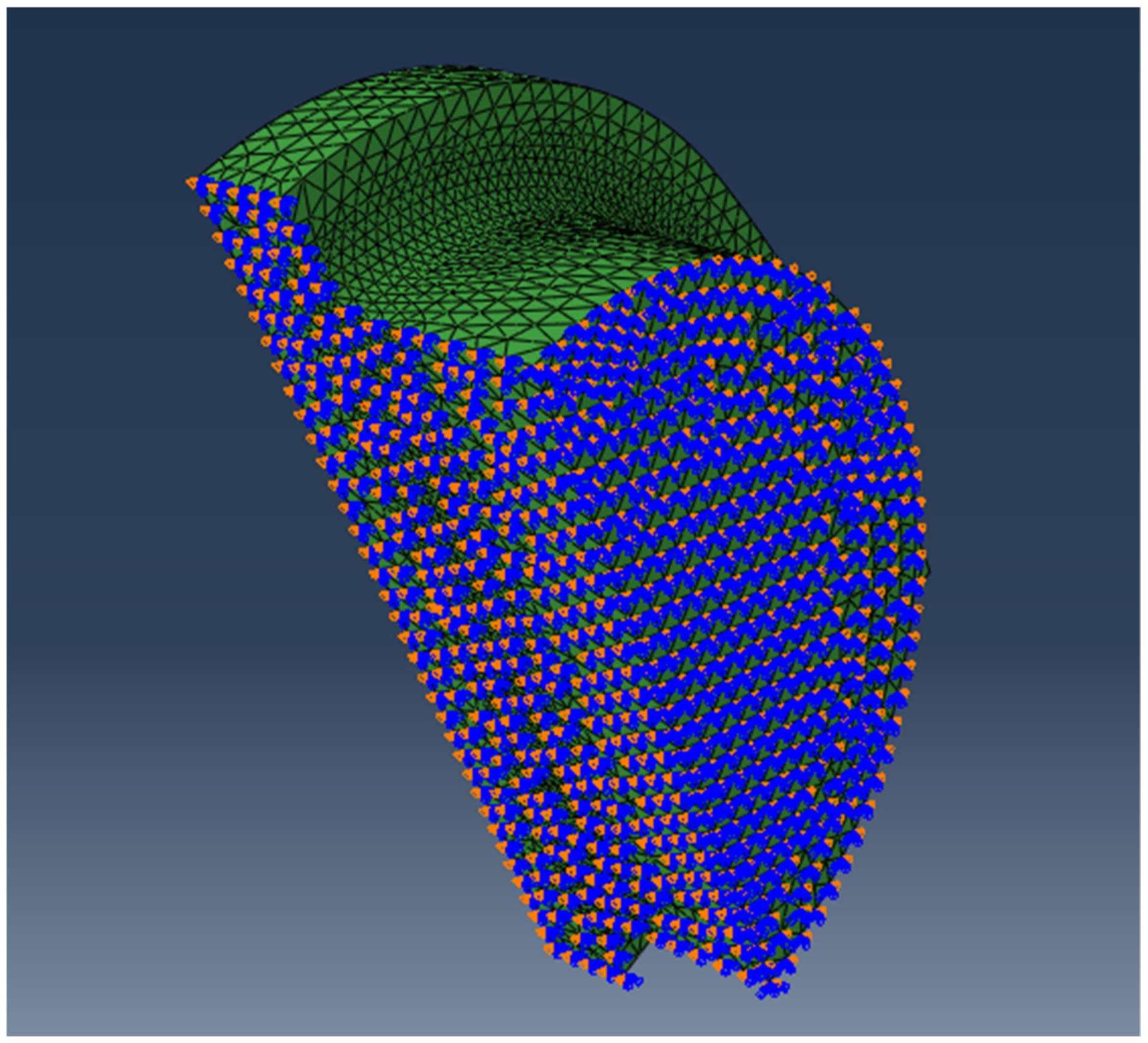
Metals 12 00913 g002
Figure 3. A quarter-pin model in the electromagnetic field ((a) Geometric model; (b) mesh model).
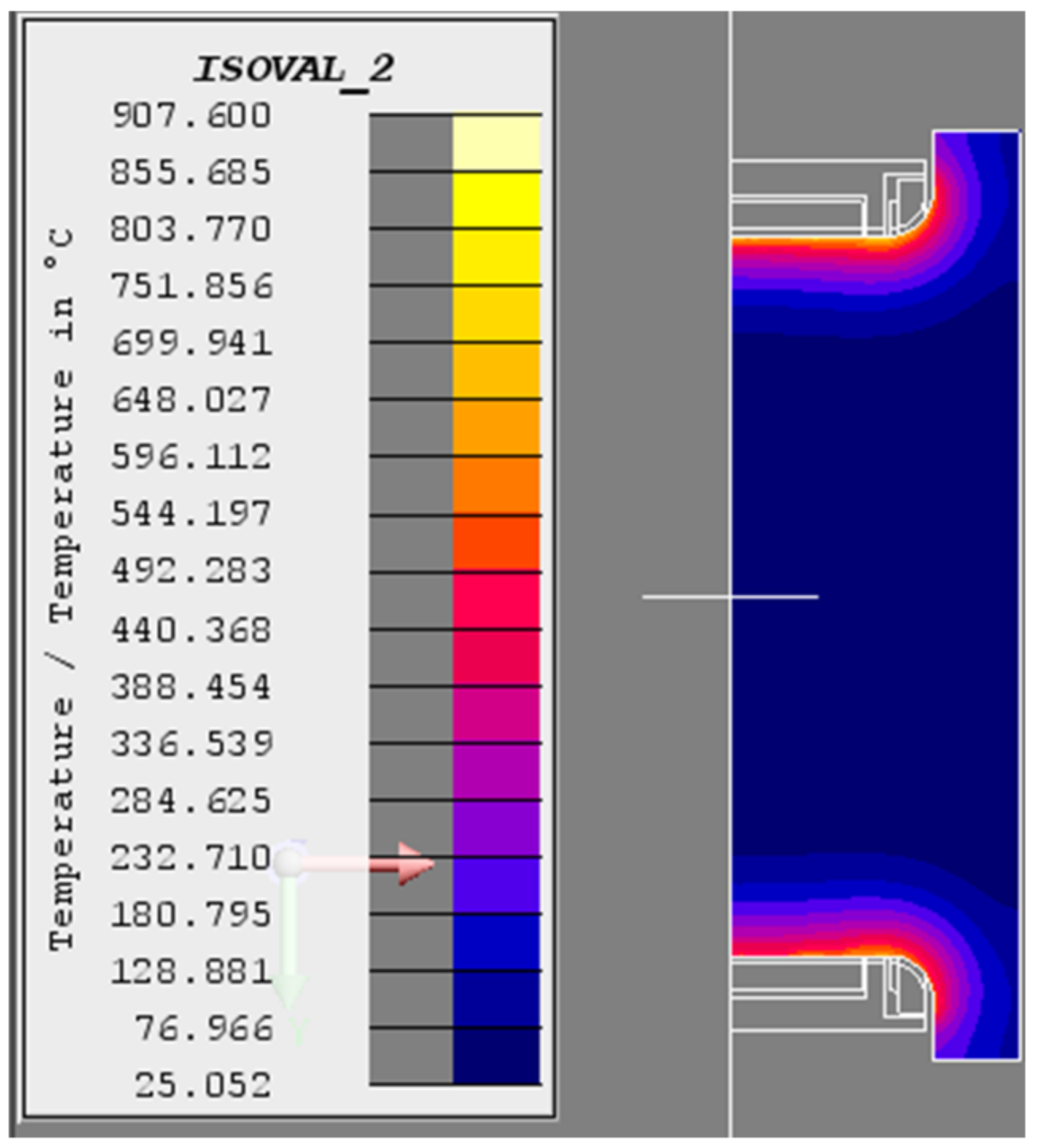
Metals 12 00913 g003
Figure 4. Temperature field of the crankshaft (T = 3 s).
Metals 12 00913 g004
Figure 5. Temperature field of the crankshaft (T = 6 s).
Metals 12 00913 g005
Figure 6. Temperature field of the crankshaft (T = 9 s).
Metals 12 00913 g006
Figure 7. 
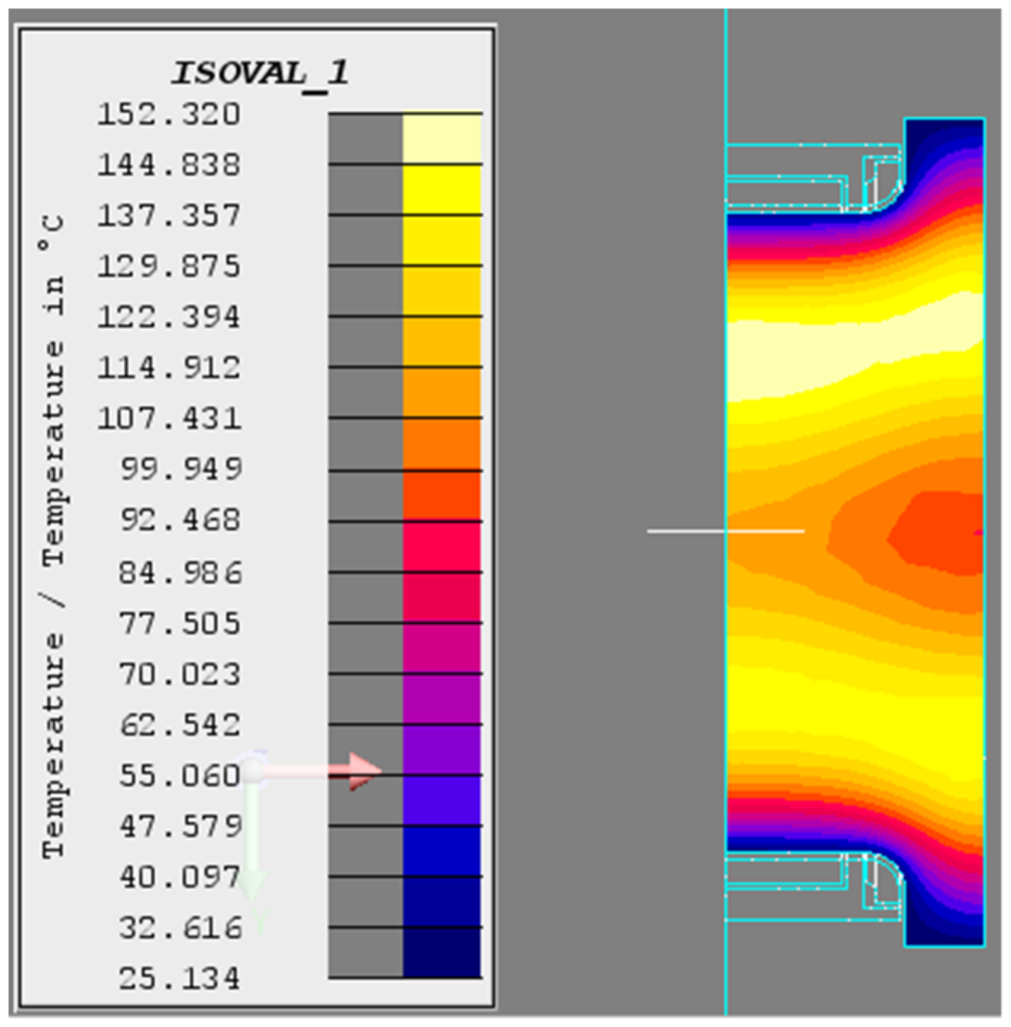
Temperature field of the crankshaft (T = 12 s).
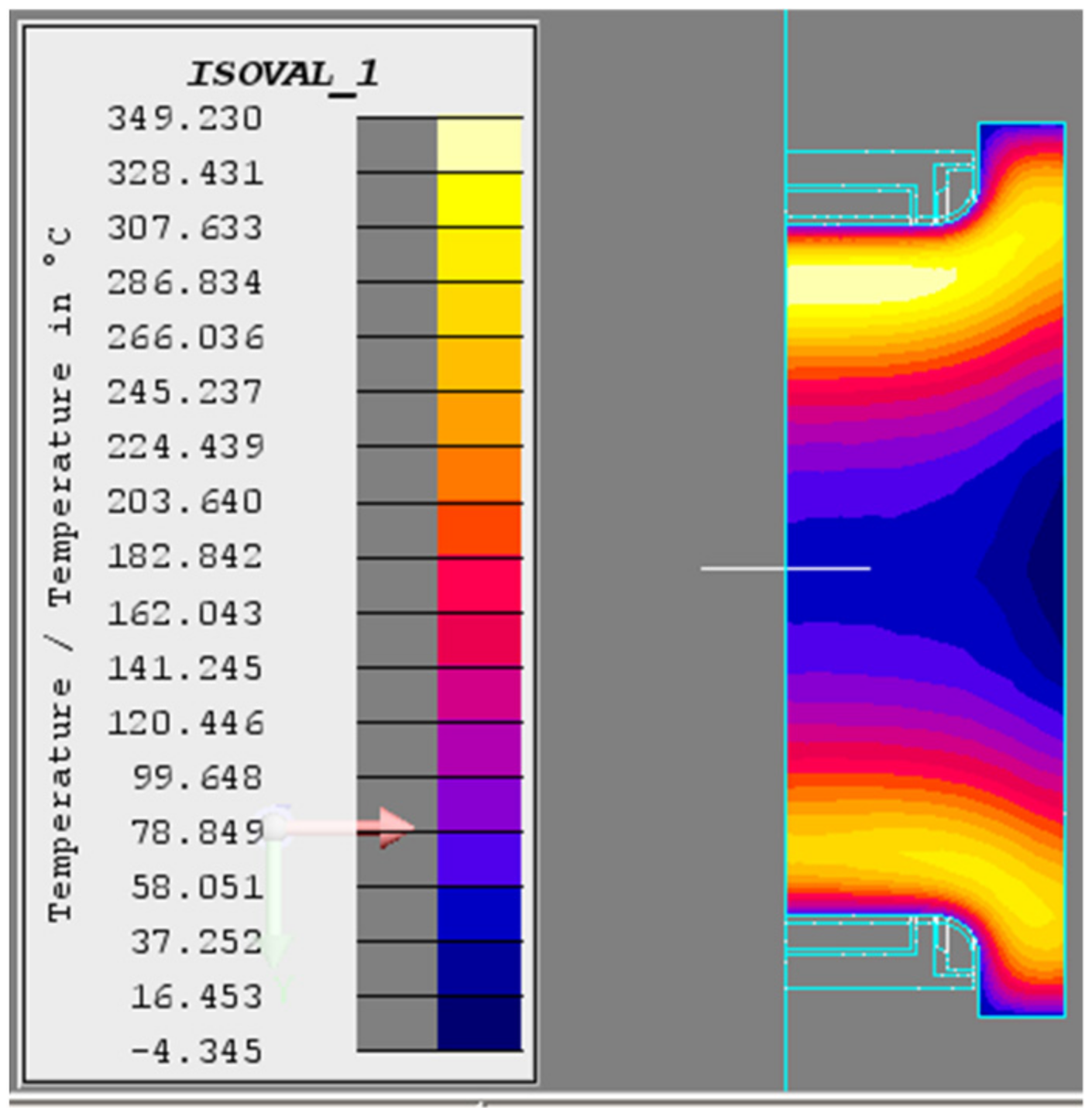
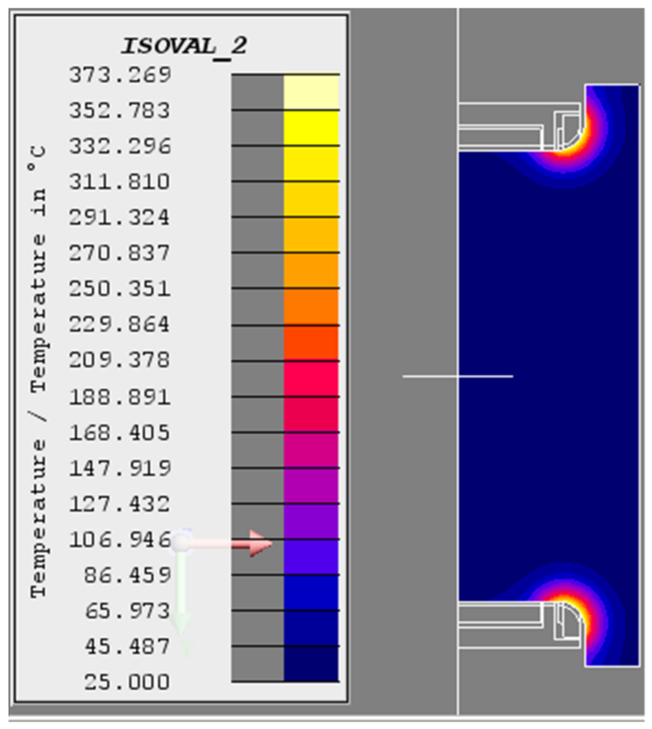
Metals 12 00913 g007
Figure 8. Temperature field of the crankshaft (T = 1 s).
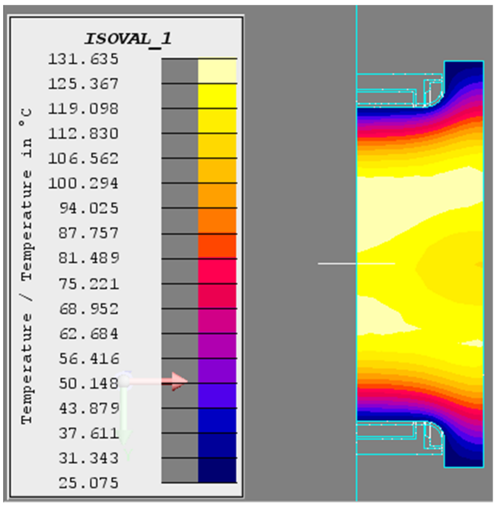
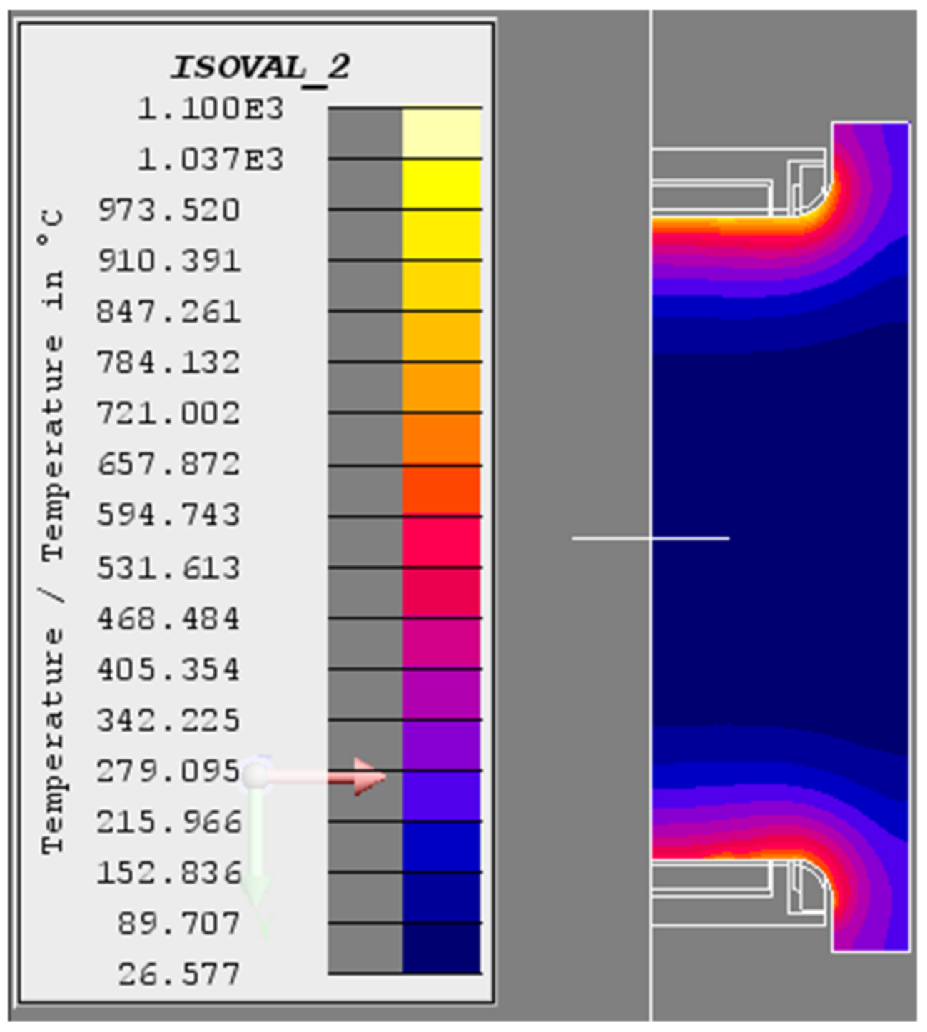
Metals 12 00913 g008
Figure 9. Temperature field of the crankshaft (T = 4 s).
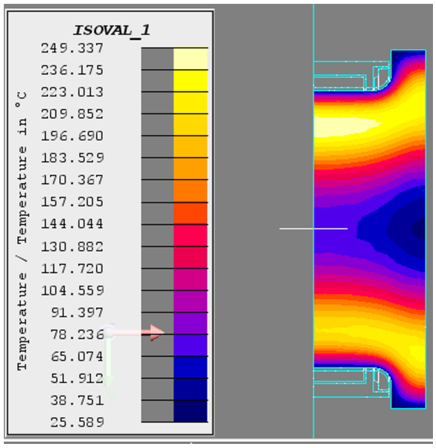
Metals 12 00913 g009
Figure 10. Temperature field of the crankshaft (T = 7 s).
Metals 12 00913 g010
Figure 11. Temperature field of the crankshaft (T = 10 s).
Metals 12 00913 g011
Figure 12. Displacement boundary conditions of the crankshaft.
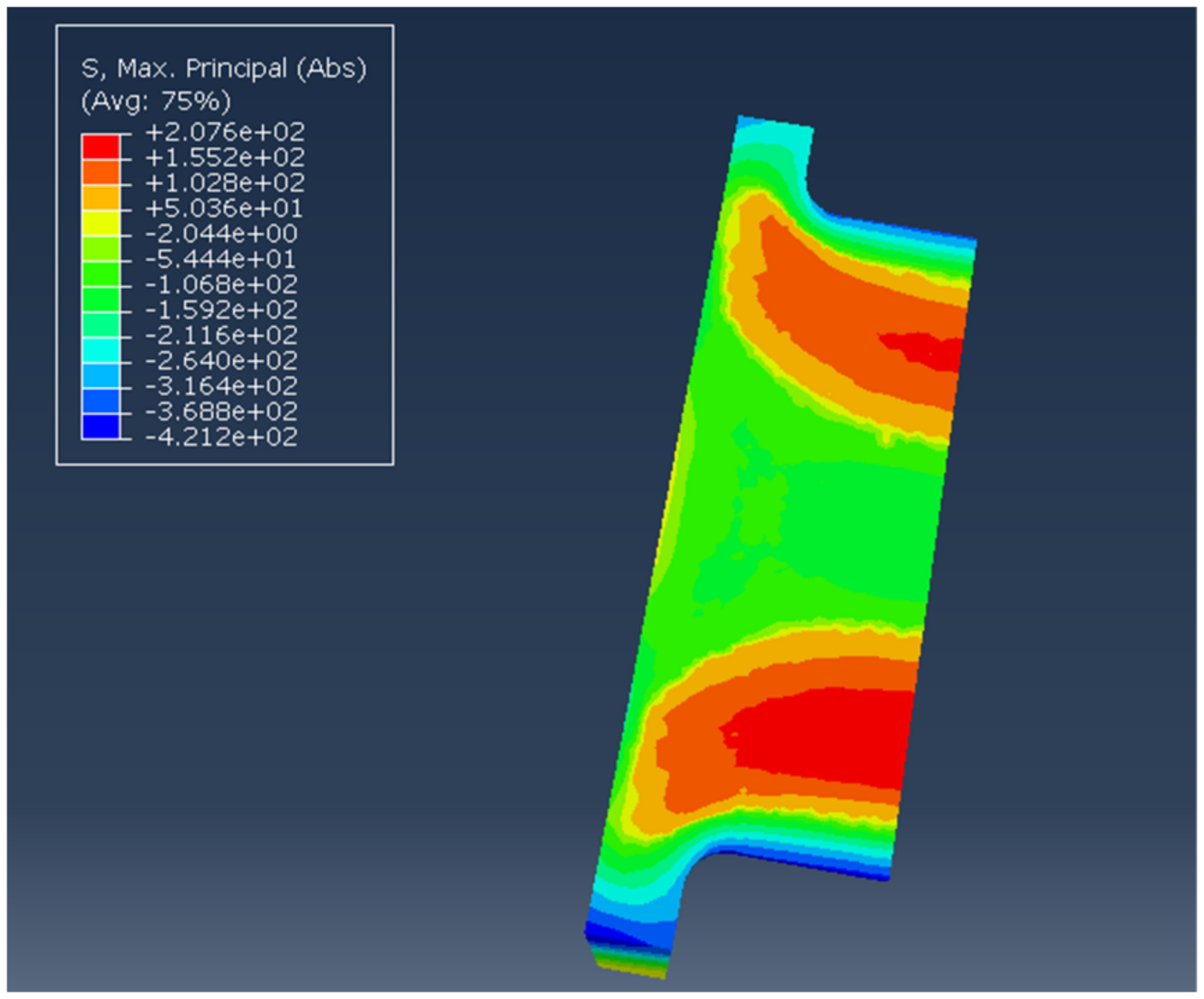
Metals 12 00913 g012
Figure 13. The residual stress field distribution of the crankshaft.
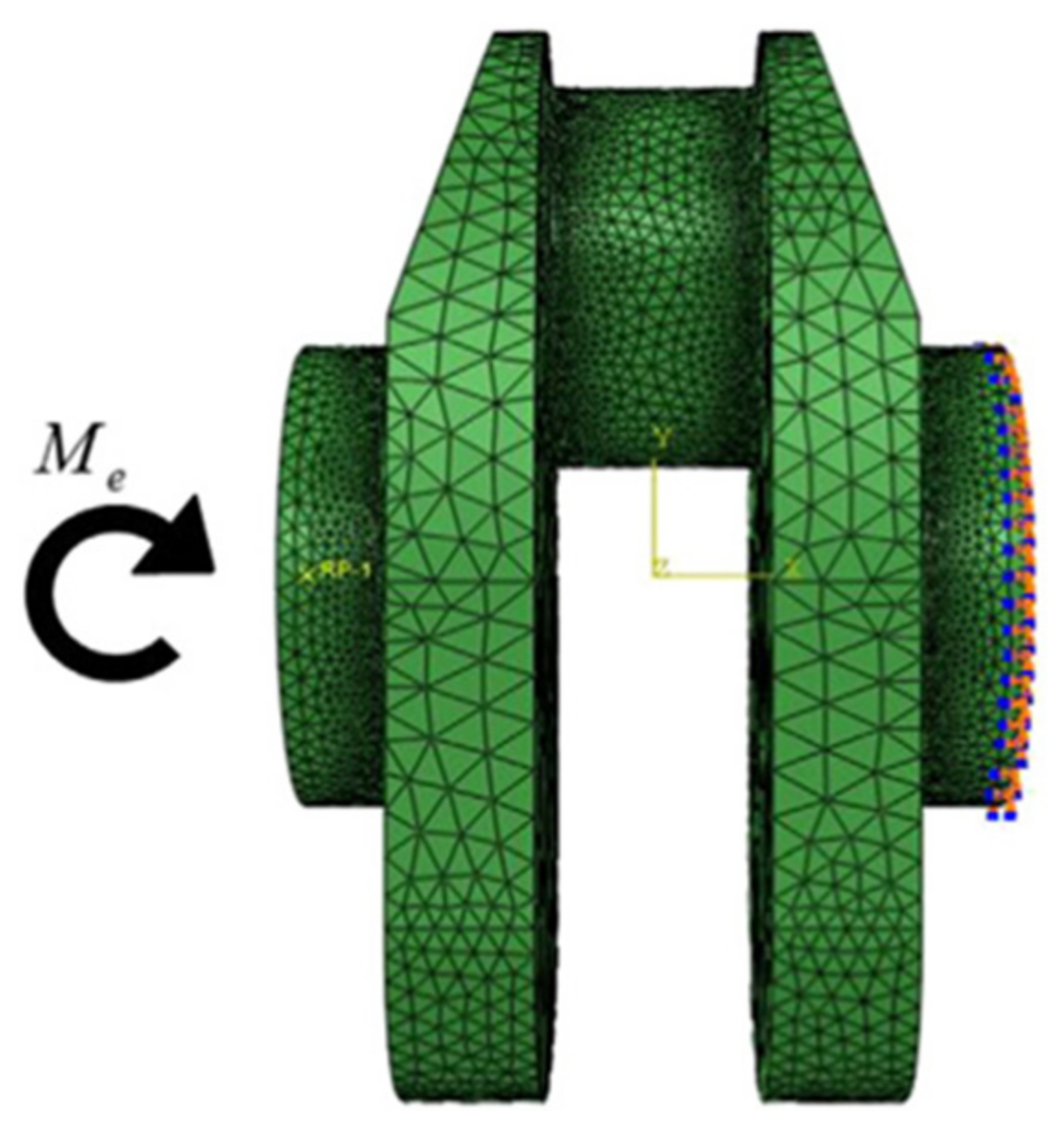
Metals 12 00913 g013
Figure 14. The finite element model of the crankshaft.
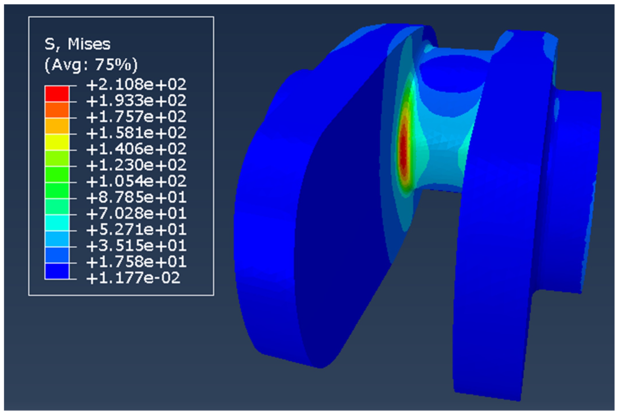
Metals 12 00913 g014
Figure 15. The Von Mises stress distribution of the crankshaft (under the given load).
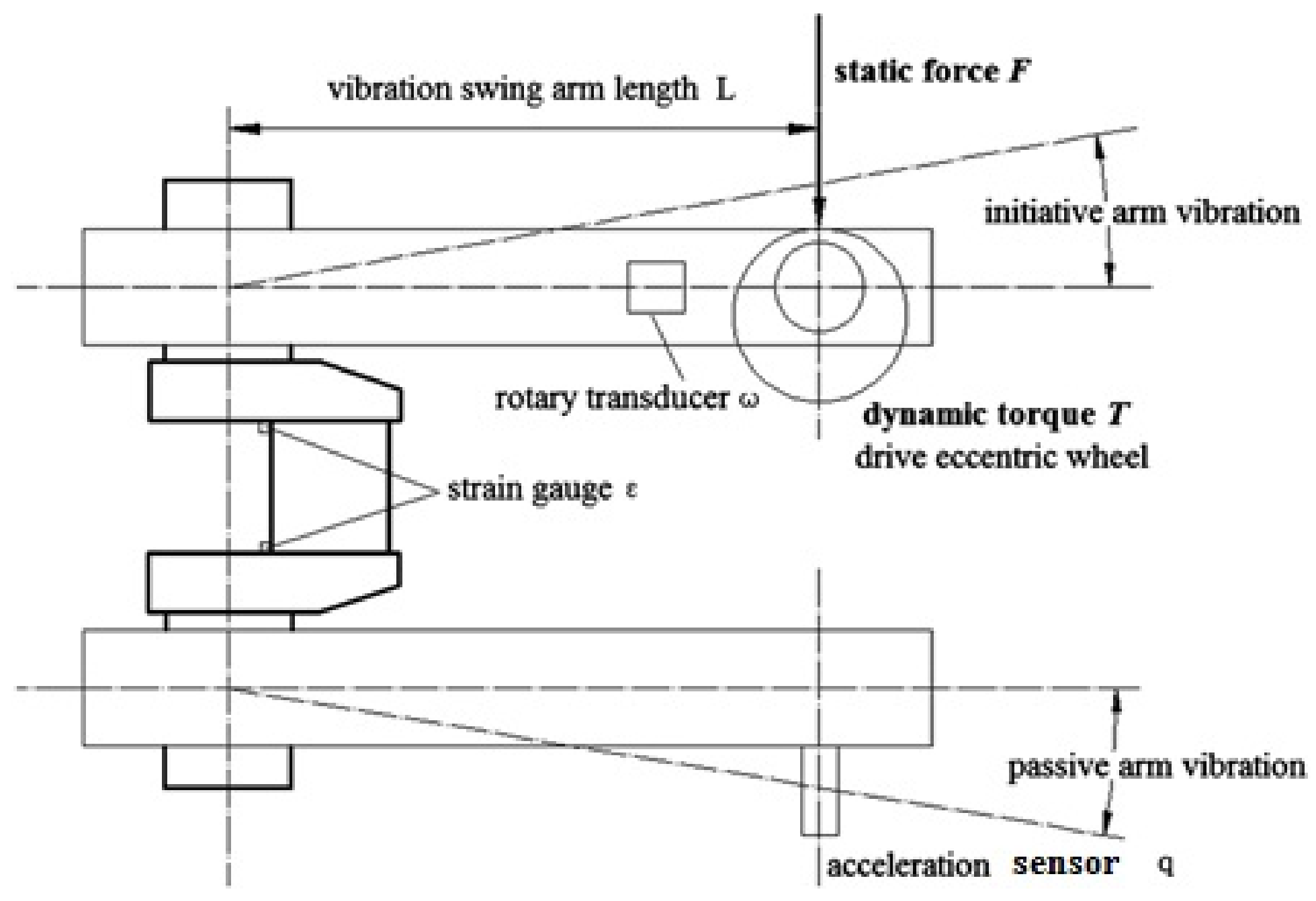
Metals 12 00913 g015
Figure 16. The bending fatigue experiment equipment.
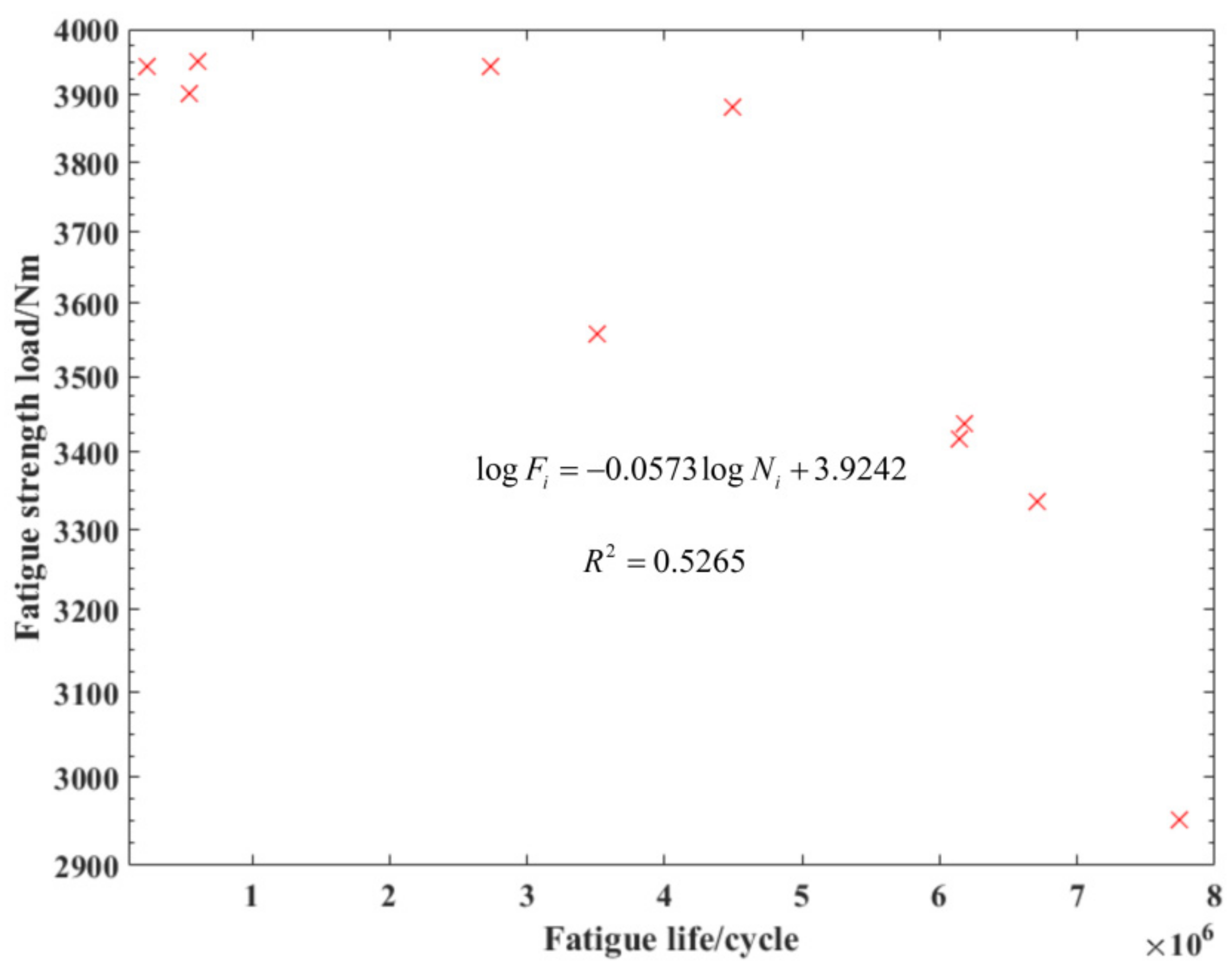
Metals 12 00913 g016
Figure 17. Fatigue test results of the crankshaft.
Metals 12 00913 g017
Table 1. Basic parameters of the material.
Temperature (°C)Relative Permeability (Mur)Volumetric Heat Capacity (J·m3·°C)Heat Conductivity (m·°C)Electrical
Resistivity (Ω·m)
252003,685,27038.51.8 × 10−7
1001943,795,04435.52.0 × 10−7
2001884,085,16135.03.2 × 10−7
3001814,390,96033.54.2 × 10−7
4001704,759,48732.55.0 × 10−7
5001585,237,78831.06.2 × 10−7
6001415,842,54528.07.7 × 10−7
7001006,845,19324.59.7 × 10−7
76018,429,07520.01.0 × 10−6
80016,241,43621.01.2 × 10−6
90015,363,24423.01.2 × 10−6
100015,308,35722.51.2 × 10−6
Table 2. Parameters of the load.
Detailed ParameterValue
Current frequency8000 Hz
Fillet working time12 s
Crankpin working time4 s
Current intensity350 A
Current density (fillet coil)9.9 × 10⁷ A/m2
Current density (crankpin coil)1.15 × 10⁸ A/m2
Table 3. Parameters of the boundary condition.
ParameterValue
Convective heat transfer coefficient150.00 W/(m2·°C)
Radiative heat transfer coefficient0.8
Young’s modulus210,000 MPa
Poisson’s ratio1.35 × 10−6/K
Coefficient of thermal expansion1.35
Stefan–Boltzmann constant5.67 × 10−8 W/(m−2·K−4)
Table 4. Stress components of the maximum stress point from different sources.
ParameterFrom the Given LoadFrom the Residual Stress Field
S1170.5 MPa−72.5 MPa
S22123 MPa−75.1 MPa
S33117 MPa−323.8 MPa
S121.5 MPa75.4 MPa
S13−2.9 MPa−1.6 MPa
S23−118 MPa2.03 MPa
Table 5. The stress components of the critical plane from the residual stress and the given load.
ParameterResidual Stress FieldGiven Load
Shear stress−24.4 MPa119.2 MPa
Normal stress−157.3 MPa−118.6 MPa
Table 6. The expressions of the commonly used mean stress models.
Model TypeExpressionModel TypeExpression
Goodman σ e q = σ a 1 σ m σ b Haigh σ e q = σ a 1 σ m σ b 0.5
Gerbera σ e q = σ a 1 σ m σ b 2 Soderberg σ e q = σ a 1 σ m σ y
Table 7. Predictions based on some other methods.
Model NameResults (N·m)
Goodman2494
Haigh2956
Soderberg2082
Gerbera2683
Table 8. The median rank (failure rate) estimation of the fatigue limit load.
Load Value/N·mMedia Rank
28930.067308
30250.163462
32550.259615
32800.355769
33210.451923
33430.548077
33520.644231
33860.740385
37380.836538
37590.932692
Table 9. Errors of the predictions.
Model NameError
Goodman32%
Haigh22.8%
Soderberg24.8%
Gerbera43.2%
McDiarmid1.1%
Publisher’s Note: MDPI stays neutral with regard to jurisdictional claims in published maps and institutional affiliations.

