Article

Predictive Modeling of Blast Furnace Gas Utilization Rate Using Different Data Pre-Processing Methods

1
School of Metallurgical and Ecological Engineering, University of Science and Technology Beijing, Beijing 100083, China
2
School of Chemical Engineering, The University of Queensland, St. Lucia, QLD 4072, Australia
3
School of Mathematics, Rose-Hulman Institute of Technology, Terre Haute, IN 47803, USA
4
He Steel Group Co., Ltd., Shijiazhuang 050024, China
*
Author to whom correspondence should be addressed.
Metals 2022, 12(4), 535; https://doi.org/10.3390/met12040535
Submission received: 17 February 2022 / Revised: 12 March 2022 / Accepted: 19 March 2022 / Published: 22 March 2022
(This article belongs to the Special Issue Fundamentals of Advanced Pyrometallurgy)

Abstract

:
The gas utilization rate (GUR) is an important indicator parameter for reflecting the energy consumption and smooth operation of a blast furnace (BF). In this study, the original data of a BF are pre-processed by two methods, i.e., box plot and 3σ criterion, and two data sets are obtained. Then, support vector regression (SVR) is used to construct a prediction model based on the two data sets, respectively. The state parameters of a BF are selected as input parameters of the model. Gas utilization after one hour (GUR-1h), two hours (GUR-2h), and three hours (GUR-3h) are selected as output parameters, respectively. The simulation result demonstrates that using the 3σ criterion to pre-process the raw data leads to better prediction of the model compared to using the box plot. Moreover, the model has the best predictive effect when the output parameter is selected as GUR-1h.

1. Introduction

At present, the process of blast furnace (BF) ironmaking is mainly that in which iron ore and coke are fed into a BF from the top in a certain proportion, and then pig iron is smelted. After the iron ore and coke flow through a distribution device, reactions take place inside the BF. Meanwhile, hot air and pulverized coal of the tuyeres is blown into the BF to promote the chemical reaction inside the BF to form an upward airflow [1]; iron ore reacts with carbon monoxide under high-temperature and high-pressure conditions inside the BF to yield products such as molten iron, slag, and gas [2]. The molten iron flows out from the bottom of the BF and is pretreated and sent to the steel plant. BF gas is collected at the top of the furnace and can be recycled. As one of the main products of BF ironmaking, BF gas carries a huge amount of thermal and chemical energy, which can provide heat for the chemical reactions inside the BF and facilitate the reactions inside the BF.
The main components of BF gas are carbon monoxide, carbon dioxide, nitrogen, and hydrogen. In the field of metallurgy, the gas utilization rate (GUR) of BF is defined as the ratio of the carbon dioxide content to the total content of carbon monoxide and carbon dioxide. With the rapid development of industry, steel companies are making efforts to improve the gas utilization rate. On the one hand, more and more countries are paying attention to emission reduction and energy conservation [3]. On the other hand, GUR reflects the reduction and utilization of the main raw materials for BF production. It represents the level of BF energy consumption, the rationality of the gas flow distribution, and the smelting state of a BF [4,5]. Most importantly, it is an important index for reducing consumption, evaluating the quality of pig iron, and increasing the production of a BF [6].
However, a BF acts as a huge black box for ironmaking reactions with a time lag, dynamics, and complexity for the production of pig iron in the modern metallurgical industry [7]. These characteristics of the BF have caused the BF operators to be unable to grasp the information of the GUR, gas distribution, and other state parameters in time. Faced with the above realistic conditions, scholars have predicted and studied BF parameters such as GUR and gas distribution based on the following three methods. ① A geometric model based on mechanism analysis (conventional solution theory and metallurgical theory). For example, Meng investigated the relationship between the temperature in the hot preparation zone and the utilization rate of blast furnace gas, and performed thermodynamic and kinetic analyses of the reduction reaction in the thermal reserve zone using standard Gibbs free energy calculations and unreacted shrinkage core models, respectively [8]. ② A computational simulation method of simulation software. For instance, a computational fluid dynamics numerical simulation model of the cooling stave of BF based on a one-dimensional heat transfer mechanism was established. The model could reduce the influence of frequent forming and shedding of the slag crusts on the BF by analyzing the effects of the cooling stave material, the volume distribution of the cooling water pipes, and the nano-polymer in the cooling stave [9]; through mathematical modeling and energy exchange analysis, Guo conducted a numerical simulation to analyze the effect of natural gas injected through the tuyere on GUR [10]. Shen developed a three-dimensional CFX-based mathematical model, which predicts the in-furnace distributions of key performance indicators such as the gas utilization rate [11]. ③ A regression model on the basis of data-driven methods and machine learning. In the past few years, some new technologies such as machine learning, deep learning, etc., have been used in the field of BF ironmaking. Under the support of these technologies, some regression models were established and used to predict and improve GUR, BF state parameters, and production indicators. For example, the influence of BF top pressure on improving the gas flow distribution is obtained based on the fuzzy theory [12]. A strategy for burden distribution was constructed for improving the GUR [13]. An online sequential extreme learning model was proposed to predict GUR [14]. Prof. Wu used BF operating parameters to predict BF GUR [15]. An proposed a multi-time-scale fusion method to predict the gas utilization rate of a blast furnace [4]. Shi presented a method for recognizing the distribution features of the blast furnace gas flow center based on infrared image processing [16]. Jiang proposed a model based on the multi-layer perceptron to predict the gas utilization rate after 1, 2, and 3 h, respectively [17]. Zhang presented a model based on a TS fuzzy neural network and the particle swarm algorithm for predicting the gas utilization rate [18].
From the above analysis, the first and second methods have contributed to GUR prediction and optimization. However, the calculation and formulation of these two methods are based on some assumptions. Their boundary conditions are difficult to be determined and these operating parameters have a certain degree of lag and measurement error. Furthermore, the calculation is complicated. In recent years, with the advancement of sensors and detectors, a large amount of production data has been collected by steel plants. GUR and other parameters can be more accurately predicted and provide more reliable guidance for BF using data-driven and machine learning technologies.
When a model is built using data-driven methods, the reliability of data must be guaranteed. However, BF is a huge reactor in ironmaking, and the limitations of measurements imposed by the adverse operating conditions (high temperature and pressure) result in missing values and outliers in the collected data. Data pre-processing is essential as an important step in the process of building a model to ensure consistency and accuracy. It is worth noting that the hysteresis in the BF ironmaking process must be considered and few scholars have performed a comparative study on the prediction of blast furnace-related parameters by different data pre-processing methods. Meanwhile, few scholars have previously focused on the duration of the effect of the current BF condition on the GUR. Therefore, in this study, two data pre-processing methods were used to build two prediction models based on support vector regression (SVR) for forecasting GUR after one hour (GUR-1h), GUR after two hours (GUR-2h), and GUR after three hours (GUR-3h). Furthermore, the impact of the two data pre-processing methods on the prediction was analyzed, which is a fundamental and important step for improving the operating level and energy utilization of the BF.
The rest of this article is organized as follows. The original data are analyzed and pre-processed by two methods, the box plot and 3σ criterion, in Section 2. Section 3 calculates the correlation of each feature, obtains the best input parameters, and describes the algorithm used in this article. Section 4 shows the prediction results of the models based on two different data sets. Section 5 compares and evaluates the prediction effects of the models. Eventually, the conclusions are summarized in Section 6.

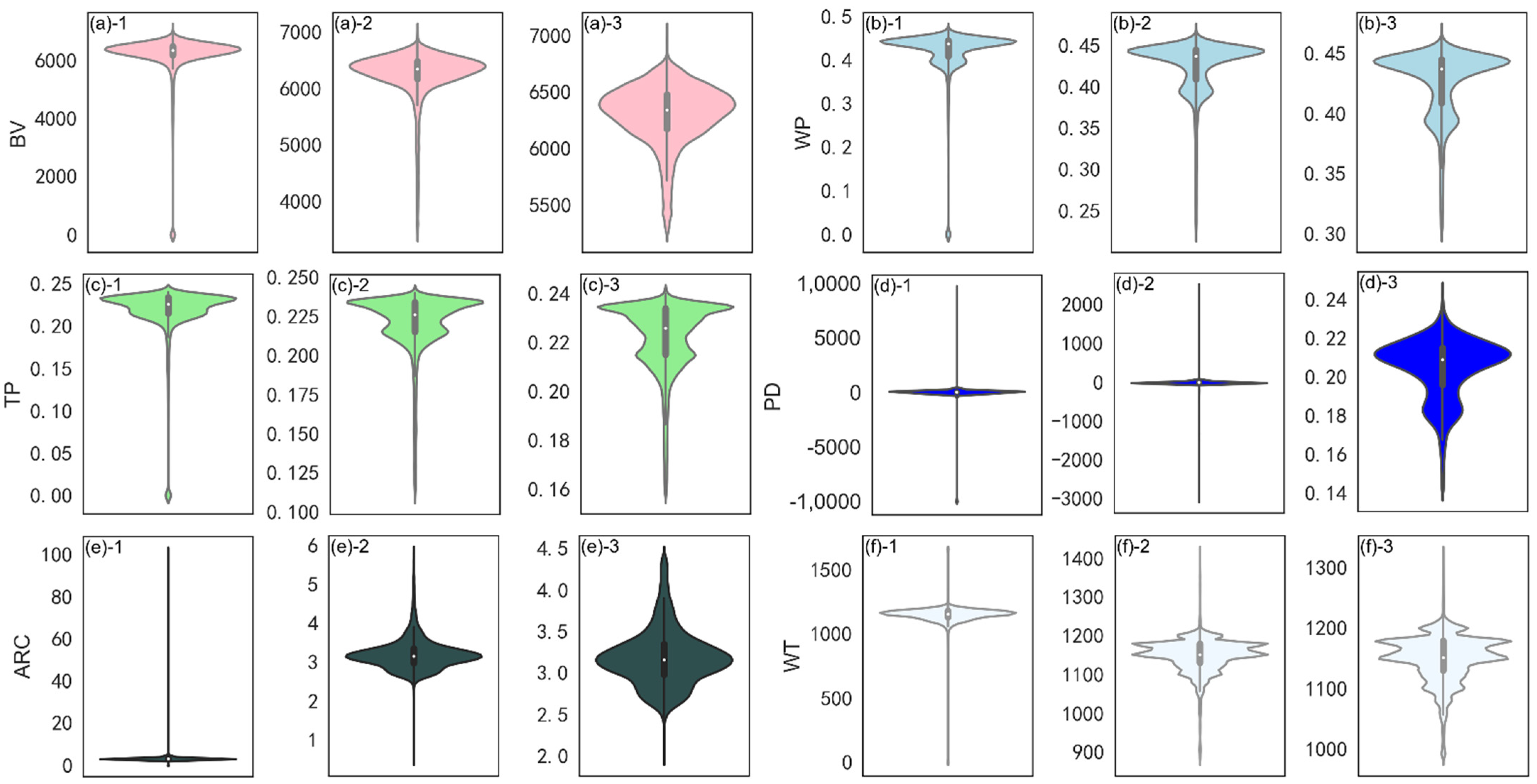
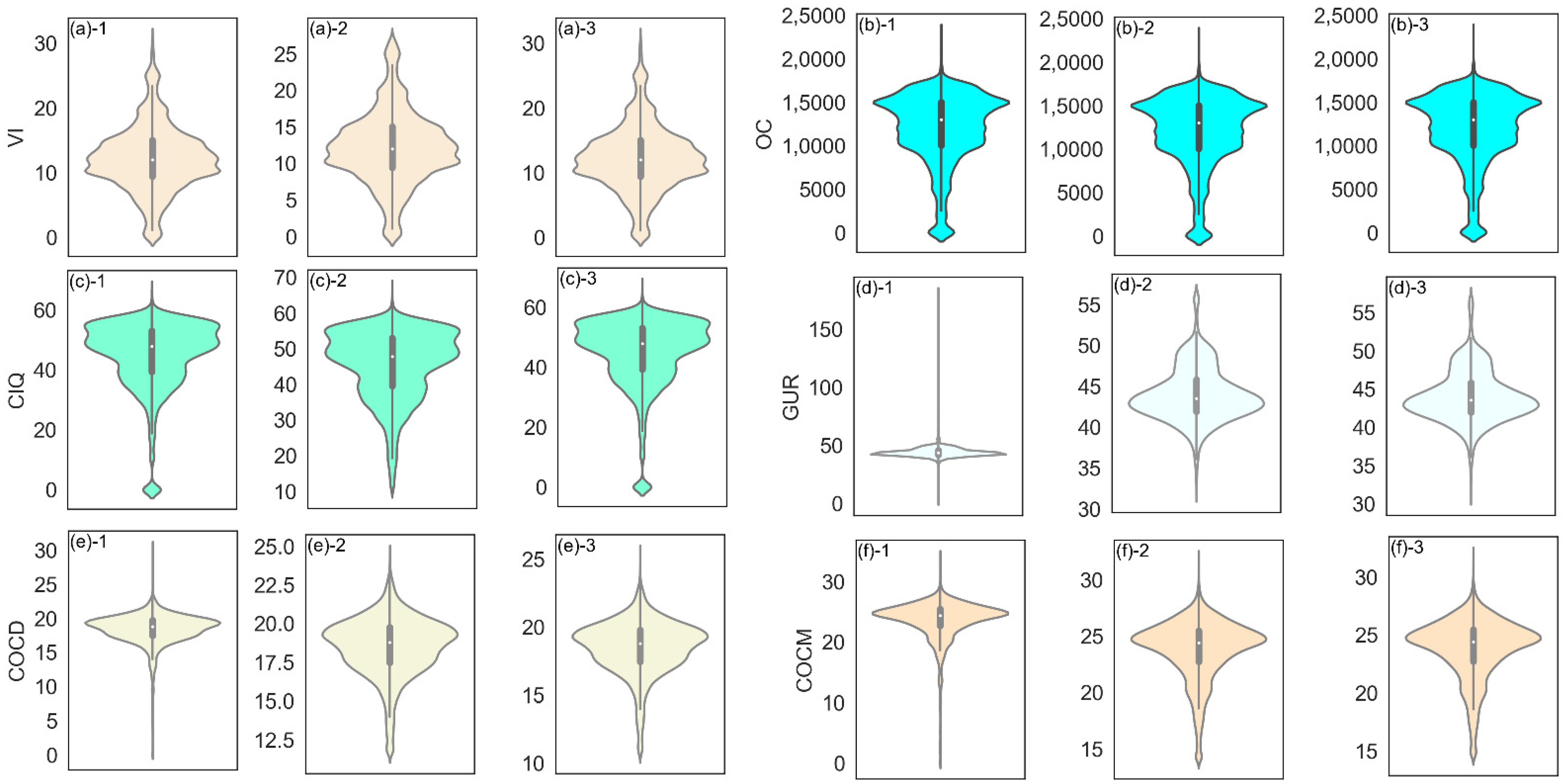
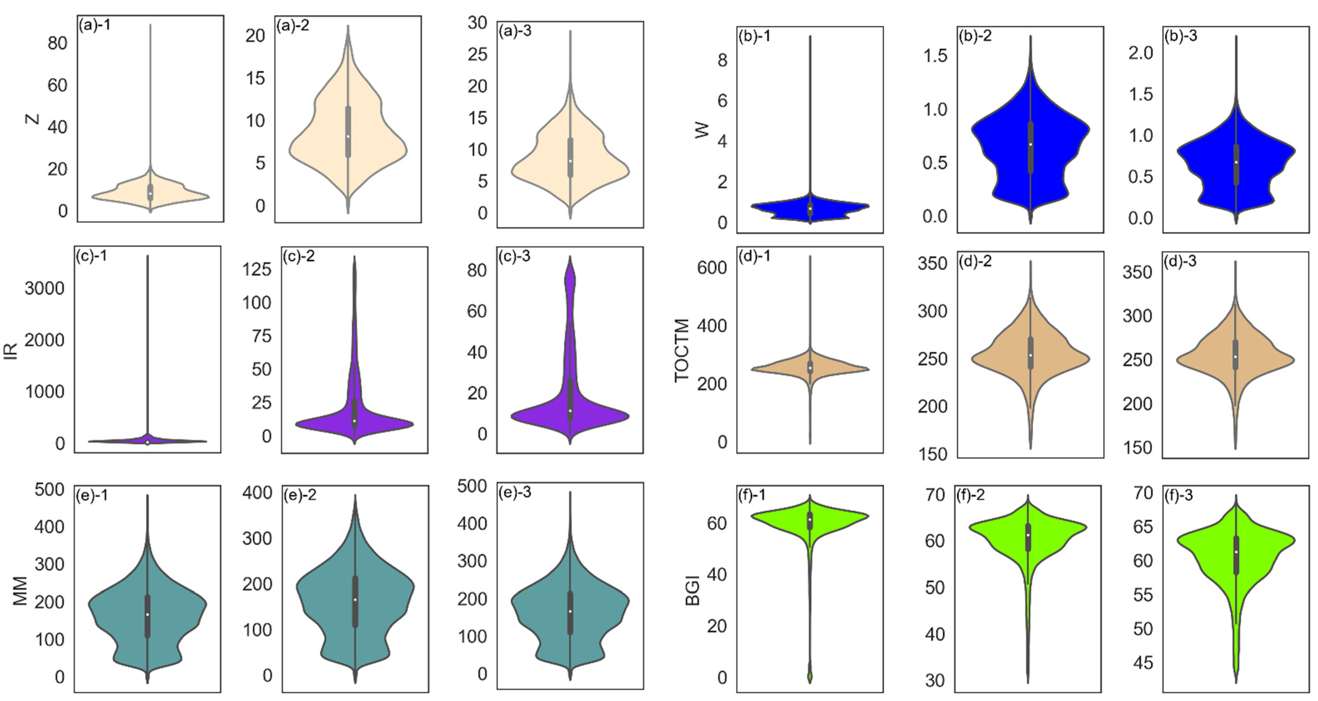
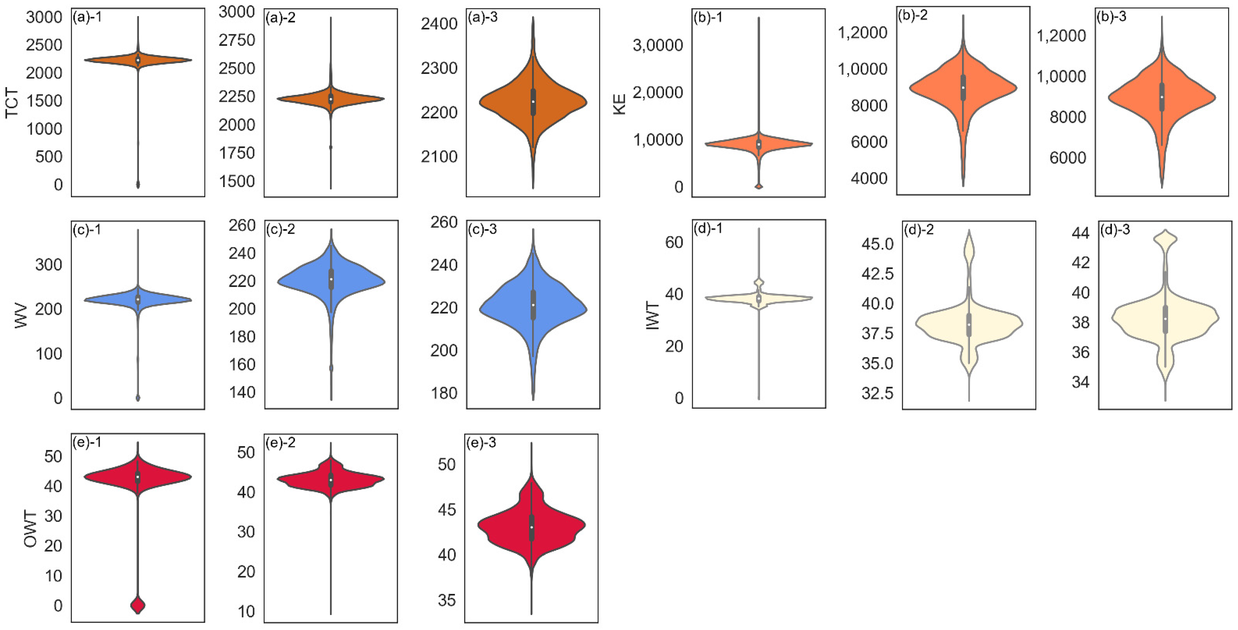
2. Pre-Processing of Raw Data

The data involved in this paper are from a BF in China with a working space of 4150 m3. The 35,198 sets of data were collected from the BF and the sampling interval was 1 h. The collected parameters of each data sample are shown in Table 1. Because these parameters are general expressions in BF ironmaking and have been described in many papers, the specific meaning of each parameter will not be repeated here [17,18,19,20,21].
In the above table, the calculation method of the GUR (ηCO) is shown as
η C O = V C O 2 V C O + V C O 2
where VCO2 and VCO represent the amount of carbon dioxide and carbon monoxide, respectively.
Ironmaking is a complex reaction process involving coking, sintering, pelleting, and ironmaking. Many related reactions are carried out under high temperature and pressure. Therefore, the collected data have a certain number of outliers and missing values. Generally, two methods are used to judge the outliers and extreme outliers: the box plot method and the 3σ criterion method [22,23].
The feature data are arranged from small to large, and Q1 and Q3 are the first quartile and the third quartile of each feature parameter in a box plot, respectively. IQR is the difference between Q3 and Q1. In this context, data within the range of Q1 + 1.5IQR or minimum to Q3-1.5IQR or maximum for each data feature in the box plot are retained, and data outside this range are considered to be outliers. Data outside of (Q1 − 3IQR, Q3 + 3IQR) are considered to be extreme outliers. Data outside the range of (μ − 3σ, μ + 3σ) are judged as extreme outliers, where μ is the mathematical expectation and σ is the standard deviation in the 3σ criterion. The values of each feature are almost all concentrated in the interval (μ − 3σ, μ + 3σ). The possibility of exceeding this range is less than 0.3%. Therefore, the data outside this range can be considered as extreme outliers. The abnormal conditions of a BF must be considered when performing predictive modeling of BF. Therefore, when the collected data are pre-processed, only extreme outliers are removed and substituted with interpolated estimates.
In order to ensure the continuity of time, extreme outliers and vacancy data are usually filled instead of completely deleted. Extreme outliers are replaced with missing values in this article. The linear interpolation method is selected, which is to construct a straight line to approximate the missing value.
The distribution of each variable can be characterized by a violin plot. It is roughly judged whether each feature has an outlier from the overall distribution of the data. It is very similar to a box plot, but it can gain insight into the distribution density of each variable. At the same time, the violin plot is particularly suitable for situations where the amount of data is huge and individual observations cannot be displayed, which is consistent with the data used in this article. Figure 1, Figure 2, Figure 3 and Figure 4 are comparison diagrams of the violin plot after replacing the extreme values in the original data with the box plot and the 3σ criterion. In Figure 1, Figure 2, Figure 3 and Figure 4, (x) − 1, (x) − 2, and (x) − 3(x = a, b, c, …, f) represent the data before a feature is processed, after it is processed by the box plot, and after it is processed by the 3σ criterion, respectively. Each feature is expressed by the same color.
The comparisons of each parameter before and after pre-processing are reflected in Figure 1, Figure 2, Figure 3 and Figure 4, where the box in each figure is the box plot. The thin black line is the whisker, and the external shape is the kernel density estimate. There are missing values, outliers, and extreme outliers in the original data, as shown in Figure 1, Figure 2, Figure 3 and Figure 4. The distribution of each characteristic parameter is uneven, and the degree of discretization of the data is relatively large. Meanwhile, Figure 1, Figure 2, Figure 3 and Figure 4 indicate that, compared to the data pre-processed by the box plot, the distribution of the data after being pre-processed by the 3σ criterion is more uniform. After the extreme outliers were pre-processed using the box plot and 3σ criterion, two different data sets were formed, which are called the box data set (BDS) and normal data set (NDS).

3. Model Construction

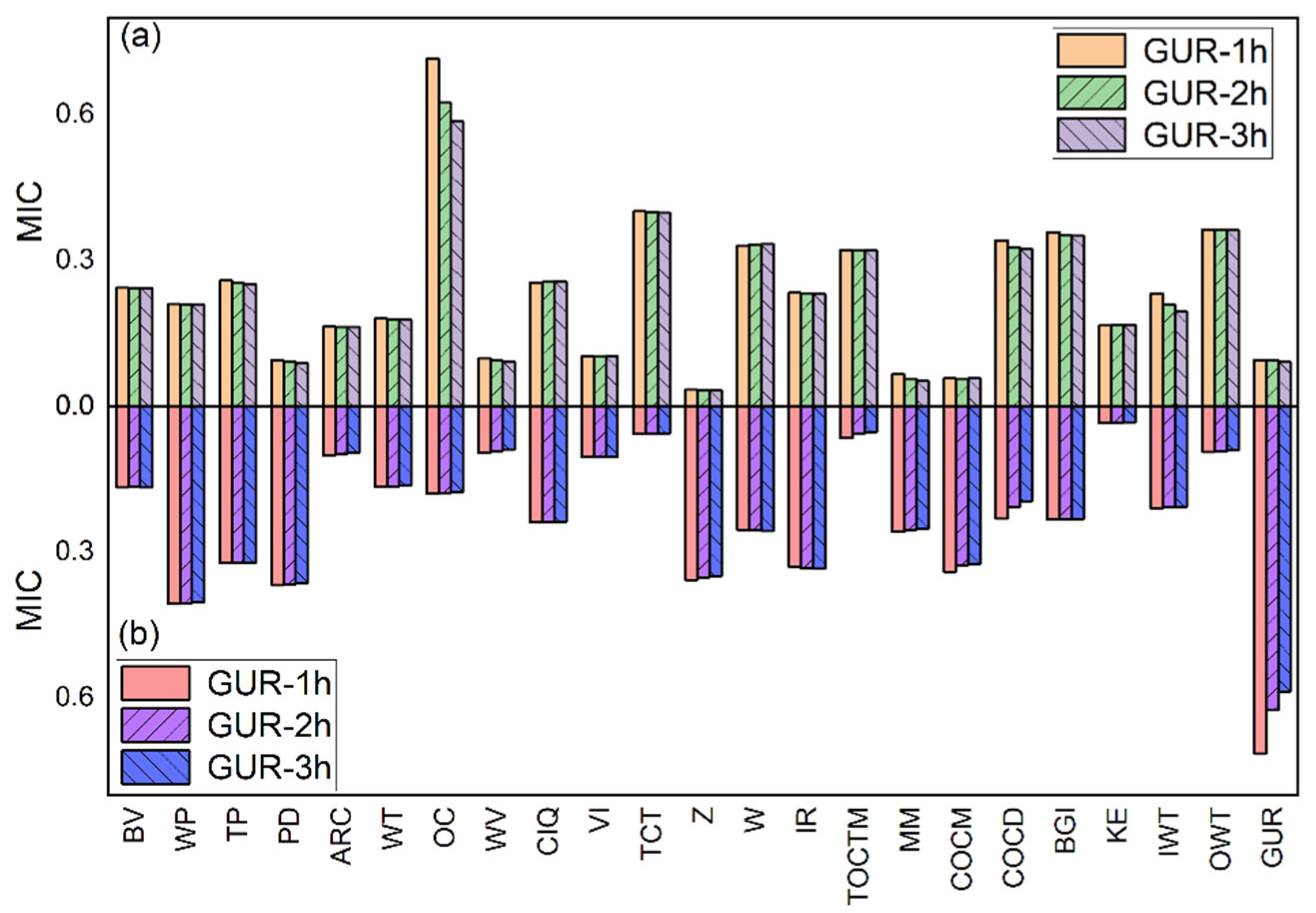
3.1. Feature Selection

The selection of input parameters in the modeling process can be determined according to the practical experience of on-site operators and the correlation between the collected parameters and GUR. For the measurement of correlation, the maximum information coefficient (MIC) is used for characterization in this paper.
If there is an association between two variables, and the scatter plots composed of these two variables are meshed, a partitioning method can always be found to describe their relevance. The correlation between two consecutive variables can be described by the MIC [24]. It mines nonlinear correlations by performing unequal interval discretization optimization on continuous variables and further makes MIC(X, Y)∈[0, 1] through standardized correction with the help of this normalization function.
y = ( y m a x y m i n ) ( x x m i n ) x m a x x m i n + y m i n
where ymin = −1 and ymax = 1. After input and output variables are standardized, the mutual information between the variables is calculated as follows:
M I C ( X ; Y ) = max | X | | Y | < B ( X ; Y ) I ( X ; Y ) log 2 ( min { | X | , | Y | ) }
I(X; Y) represents the mutual information of X and Y in Formula (3). Moreover, |X| and |Y|, respectively, represent the number of segments in which the variables X and Y are divided into the mesh division process. The value of B is generally set to 0.6 or 0.55. In this paper, the value of B is 0.6. The mutual information is calculated as follows:
I ( X ; Y ) = x = X y = Y p ( X , Y ) log 2 p ( X , Y ) p ( X ) p ( Y )
X and Y are two connected random variables, and p(X, Y) is the joint probability density distribution function in Formula (2). The MICs of the initially selected input parameters for the BDS and NDS are shown in Figure 5.
The MICs between the feature parameters and GUR-1h, GUR-2h, and GUR-3h in the BDS and NDS data sets are shown in Figure 5a,b, respectively. The characteristic parameters with the values of MIC greater than 0.15 are finally selected as input variables based on expert experience and the above calculation results. Therefore, 16 input parameters are finally selected, respectively, for the BDS and NDS, and the selected parameters are shown in Table 2.

3.2. Method of Model Construction

Traditional regression prediction generally attempts to obtain a function such as a form f(x) = wTx + b for a data set: D = {(xm,ym). The optimization process is to reduce directly the difference between the predicted value (f(x)) and the true value (y). The loss function is shown in Equation (5).
J ( θ ) = 1 2 i = 1 m ( h θ ( x i ) y i ) 2
where yi represents the actual value, and hθ(xi) means the predicted value.
The loss is calculated when |f(x)-y| > ε for the SVR algorithm. If the feature vector mapping x from the low-dimensional space to the high-dimensional space is expressed as Φ(x), then the hyperplane model divided by the high-dimensional space is as shown in Equation (6):
f ( x ) = w T Φ ( x ) + b
where w is the normal vector and b is the displacement term., An interval band with a width of 2ε is constructed by taking f(x) as the center. If the training sample falls into this interval band, the prediction is considered to be correct. Then, the kernel function [18] is introduced into SVR as shown in Equation (7).
f ( x ) = i = 1 m ( a ^ i a i ) · k ( x i , x ) + b
b = y i + ε i = 1 m ( a ^ i a i ) · k ( x i , x j )
where k(xi,xj) is a kernel function.
The choice of the kernel function, such as the rbf function, linear kernel function, polynomial kernel function, or sigmoid kernel function, is very important for the prediction result of SVR. The SVR prediction model can be finally determined by the grid search [25].
The actual data of the BF have different magnitudes, which has a significant impact on the predictive performance of a model. Therefore, in addition to handling extreme outliers, the data also need to be standardized before modeling. The process of data normalization ensures that each feature has an average of 0 and a variance of 1. It makes all features in the same magnitude, which also reduces the impact of anomaly data on the built model. At the same time, the output of the model can be restored to the original output parameters through the de-standardization method.

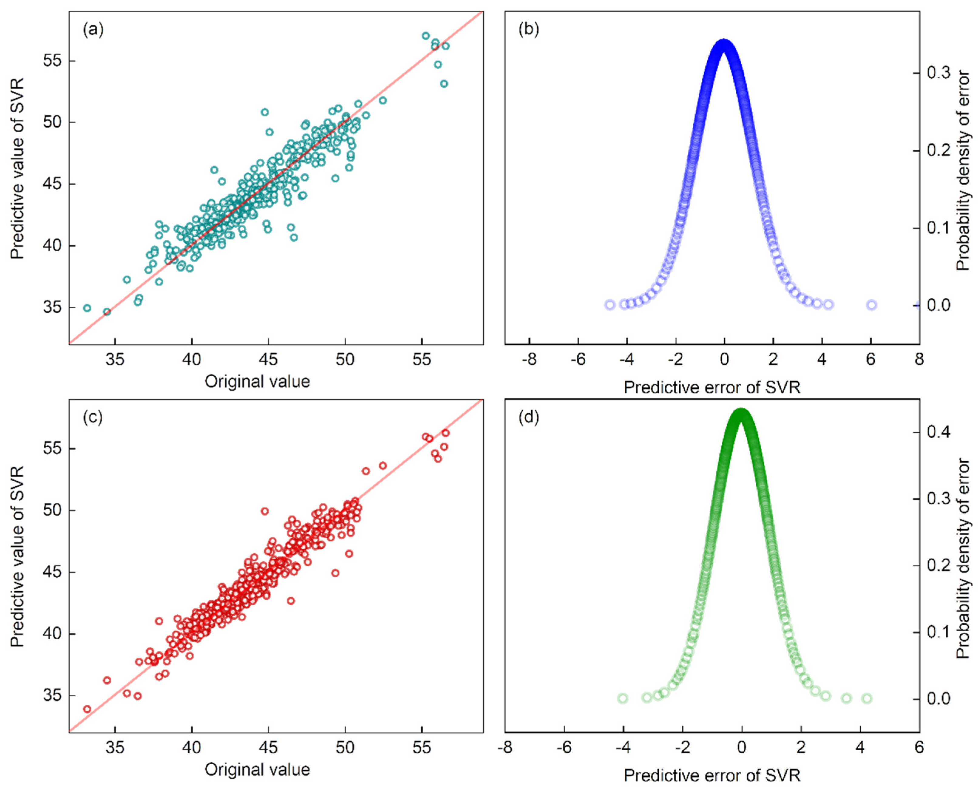
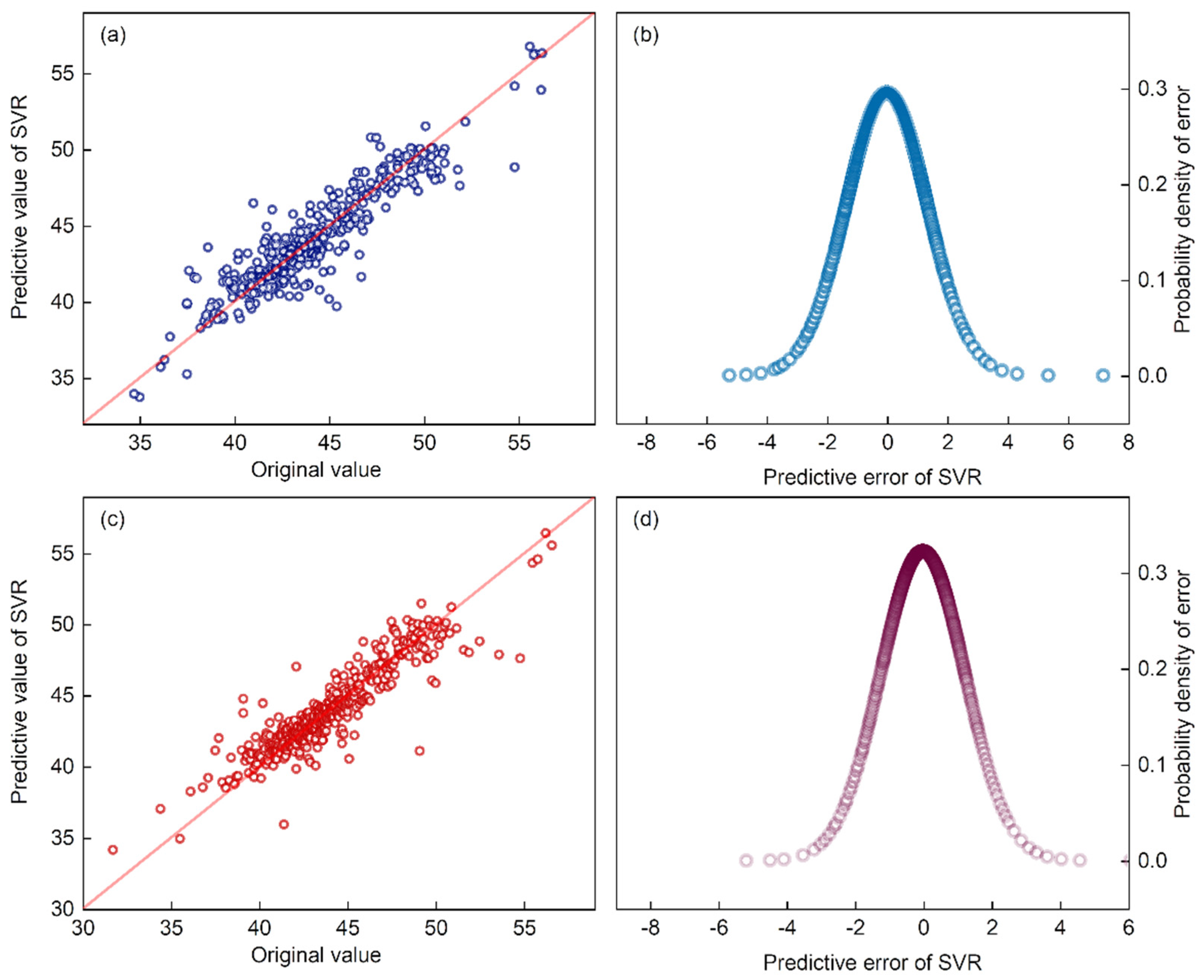
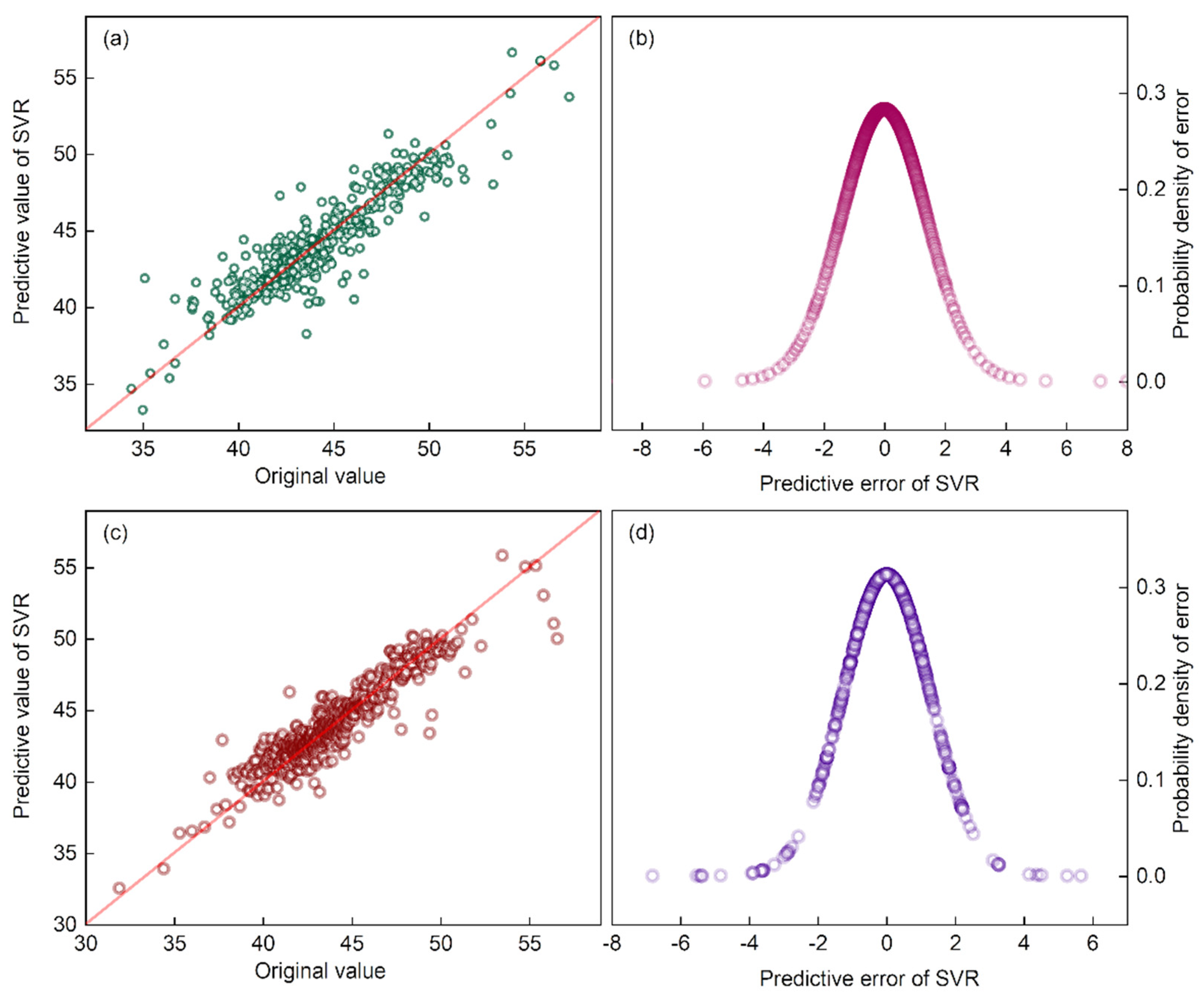
4. Comparison of the Prediction Results Based on Two Data Sets

In order to achieve an accurate prediction, the SVR model was established in this paper. After the model is optimized through the grid search, the best hyperparameters of the model are obtained, as shown in Table 3. C is the penalty parameter and γ is a parameter in the RBF kernel function [25,26].
Due to the massive volume of test data, the 100 sets of measured values in the test set of BDS and NDS are marked in black and the correspondingly predicted values are marked in red and blue when the predicted parameter is the GUR-1h. The results are expressed in Figure 6a,b, respectively.
Figure 6a,b show the comparison among the original values and the predicted values of the SVR model based on BDS and NDS when the predicted parameter is GUR-1h, respectively. Figure 6 shows that the black points basically coincide with the red points and blue points, which indicates that the predicted values of the SVR model based on BDS and NDS are not of much difference from the true values. In the process of testing, the 8800 sets of data, which are 25% of the total sample, are selected as the test data. After sorting according to the actual values, the forecasting bias of the SVR model is as shown in Figure 7.
Figure 7a,c show the degree of the prediction deviation of the SVR models constructed based on BDS and NDS when the predicted parameter is the GUR-1h, respectively. Figure 7b,d are the images of the predicted deviation probability density function of the SVR models constructed based on BDS and NDS when the predicted parameter is GUR-1h, respectively. The horizontal axis is the actual value, and the vertical axis is the predictive value by the SVR models constructed based on BDS and NDS in Figure 7a,c. If the original value is very close to the predicted value, the image is in complete and exact accordance with the diagonal. It is observed that the prediction results of the SVR models constructed based on BDS and NDS fluctuate around the diagonal line, and the fluctuation range is narrow. Figure 7b,d indicate that the values of the predicted error of the two models are basically within the range of ±2.
When the output parameter is the GUR-2h, the predicted results of the SVR model constructed using the BDS and the NDS, respectively, are as shown in Figure 8.
Figure 8a,b show the comparisons among the original values and the predicted values of the SVR model based on BDS and NDS when the predicted parameter is the GUR-2h, respectively. The predictive errors of the SVR model constructed using the BDS and the NDS are shown in Figure 9.
Compared to Figure 9c, the data in Figure 9a fluctuate slightly. In Figure 9b,d, the range of prediction errors gradually expands. When the output parameter is the GUR-3h, the prediction results of the SVR model constructed using the BDS and the NDS are as shown in Figure 10.
In Figure 10a,b, the fit between the predicted values and the true value gradually deteriorates. Figure 11 represents the range of errors between the predicted values and the actual values. Compared to Figure 7 and Figure 9, the prediction errors in Figure 11 are significantly larger.

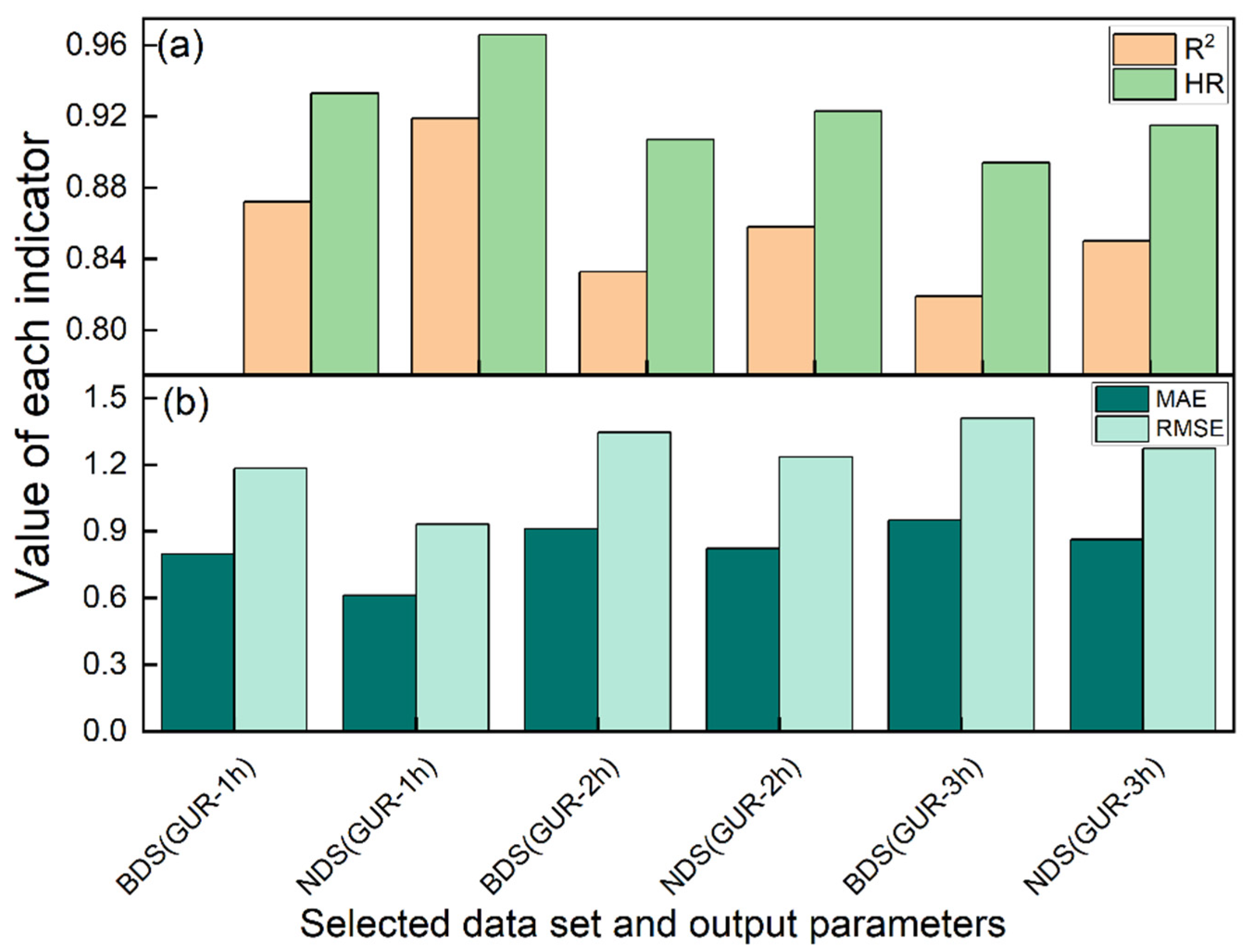
5. Evaluation Indicators and Analysis

In total, 35,198 sets of data collected by the online detection system of BF in China are used to predict the model in this paper. Moreover, 75% of the data are used for training the model and the remaining data are used for testing the model [19,20,21]. The evaluation of the prediction results of a model should be characterized by multiple aspects and multiple scales [27]. Generally, the characterization index is mainly the coefficient of determination (R2), mean absolute error (MAE), root mean square error (RMSE), or hit rate (HR) [19,20,21,27]. The reliability of the model can be represented by these parameters within the acceptable range of the processing process, and the calculation methods are shown in Equations (9)–(12), respectively:
R 2 = 1 i = 1 ( h ( x i ) y i ) 2 / i = 1 n ( y ¯ y i ) 2
M A E = 1 n · i = 1 n | h ( x i ) y i |
R M S E = 1 n · i = 1 n ( h ( x i ) y i ) 2
{ H R = 1 n · i = 1 n H R i × 100 % H R i = { 1 ,   | h ( x i ) y i | c 0 ,   | h ( x i ) y i | > c
The range of R2 is [0, 1]. In general, the larger the result, the better the fitting effect of the model. n is the total number of samples in the test set, and h(xi) and yi are the predicted and original values of the output parameters, respectively. c is the boundary value of the hit rate. In this paper, the value of c is selected as 2%. At this time, the R2 and HR of the two models are as shown in Figure 12a, and the MAE and RMSE of the two models are shown in Figure 12b.
High values of R2 and HR, and low values of MAE and RMSE, represent higher prediction accuracy of the model, as in Figure 12. Compared with the other two cases, when the output parameter is selected as GUR-1h, for NDS and BDS, the predicted accuracy of SVR is always the highest. When the selected data set is NDS and the output parameter is GUR-1h, the predictive accuracy and the hit rate of the SVR model are 91.9% and 96.6%, respectively. In this case, the SVR model obtains the best prediction effect. Moreover, regardless of whether the data are advanced using the 3σ criterion or the box plot, the predictive effect of the SVR model is strong.

6. Conclusions

GUR is an important indicator reflecting the energy consumption and smooth operation of the BF. This paper analyzes the impact of two data processing methods, the box plot and 3σ criterion, in predicting the blast furnace gas utilization rate. The box plot and 3σ criterion are selected to judge extreme outliers in this article, and linear interpolation is used to process extreme outliers and missing values. The simulations show that the prediction model using the SVR algorithm is more accurate based on the processed blast furnace data with the 3σ criterion. Hysteresis in blast furnace smelting must be taken into account, and the GUR-1h, GUR-2h, and GUR-3h are selected as output parameters, respectively. The experimental results show that the prediction of the gas utilization rate after one hour is most accurate using the parameters in the current state in the blast furnace smelting process. Moreover, as the time interval between predictions becomes longer, the prediction accuracy decreases.
This study is a first step; there are several avenues for further exploration. One natural extension is missing value handling. Other methods could be considered for replacing missing values. Another avenue for future work is extension to supply side applications, such as the development of a blast furnace gas utilization rate forecasting system that can be applied to actual production, to reduce energy consumption for blast furnace production, and to provide ancillary services for subsequent processes.

Author Contributions

Formal analysis, K.L.; Investigation, J.Z., L.J. and L.H.; Validation, Z.W.; Writing—original draft, D.J. All authors have read and agreed to the published version of the manuscript.

Funding

This work was supported by the National Natural Science Foundation of China (Project No.: 51904026) and China Postdoctoral Science Foundation (Project No.: BX20200045 and 2021M690370).

Conflicts of Interest

The authors declare no conflict of interest.

References

  1. Ling, J.; Chuanhou, G.; Zhonghang, X. Constructing Multiple Kernel Learning Framework for Blast Furnace Automation. IEEE Trans. Autom. Sci. Eng. 2012, 9, 763–777. [Google Scholar] [CrossRef]
  2. Jianqi, A.; Jialiang, Z.; Min, W.; Jinhua, S.; Takao, T. Soft-sensing method for slag-crust state of blast furnace based on two-dimensional decision fusion. Neurocomputing 2018, 315, 405–411. [Google Scholar]
  3. Hao, P.; Haibin, Y.; Mingzhe, Y. Modeling and analysis of energy using efficiency of the blast furnace. Manuf. Autom. 2011, 33, 142–144. [Google Scholar]
  4. Jianqi, A.; Xiaoling, S.; Min, W.; Jinhua, S. A multi-time-scale fusion prediction model for the gas utilization rate in a blast furnace. Control Eng. Pract. 2019, 92, 104120. [Google Scholar]
  5. Limin, Z.; Changchun, H.; Junpeng, L.; Xinping, G. Operation status prediction based on top gas system analysis for blast furnace. IEEE Trans. Control Syst. Technol. 2017, 25, 262–269. [Google Scholar] [CrossRef]
  6. Ling, J.; Chuanhou, G. Binary coding SVMs for the multiclass problem of blast furnace system. IEEE Trans. Ind. Electron. 2013, 60, 3846–3856. [Google Scholar] [CrossRef]
  7. Ray, H.; Pal, S. Simple method for theoretical estimation of viscosity of oxide melts using optical basicity. Ironmak. Steelmak. 2004, 31, 125–130. [Google Scholar] [CrossRef]
  8. Meng, F.; ZOU, Z. Influence of thermal reserve zone temperature in blast furnace on gas utilization rate. J. Northeast. Univ. 2018, 39, 985. [Google Scholar]
  9. Weiching, C.; Wentung, C. Numerical simulation on forced convective heat transfer of titanium dioxide/water nanofluid in the cooling stave of blast furnace. Int. Commun. Heat Mass Transf. 2016, 71, 208–215. [Google Scholar]
  10. Tonglai, G.; Mansheng, C.; Zhenggen, L.; Jue, T.; JunIchiro, Y. Mathematical modeling and exergy analysis of blast furnace operation with natural gas injection. Steel Res. Int. 2013, 84, 333–343. [Google Scholar] [CrossRef]
  11. Shen, Y.; Guo, B.; Chew, S.; Austin, P.; Yu, A. Three-dimensional modeling of flow and thermochemical behavior in a blast furnace. Metall. Mater. Trans. B 2015, 46, 432–448. [Google Scholar] [CrossRef]
  12. Jianqi, A.; Junyu, Y.; Min, W.; Jinhua, S.; Takao, T. Decoupling control method with fuzzy theory for top pressure of blast furnace. IEEE Trans. Control Syst. Technol. 2019, 27, 2735–2742. [Google Scholar] [CrossRef]
  13. Min, W.; Kexin, Z.; Jianqi, A.; Jinhua, S.; Kangzhi, L. An energy efficient decision-making strategy of burden distribution for blast furnace. Control Eng. Pract. 2018, 78, 186–195. [Google Scholar]
  14. Yanjiao, L.; Sen, Z.; Yixin, Y.; Wendong, X.; Jie, Z. A novel online sequential extreme learning machine for gas utilization ratio prediction in blast furnaces. Sensors 2017, 17, 1847. [Google Scholar]
  15. Guimei, C.; Anwei, C.; Xiang, M. An identification method of center gas-flow distribution pattern based on sensed infrared image processing. Inf. Control 2014, 43, 110–115. [Google Scholar] [CrossRef]
  16. Lin, S.; You-bin, W.; Guangsheng, Z.; Tao, Y. Recognition of blast furnace gas flow center distribution based on infrared image processing. J. Iron Steel Res. Int. 2016, 23, 203–209. [Google Scholar]
  17. Jiang, D.; Wang, Z.; Zhang, J.; Jiang, D.; Li, K.; Liu, F. Machine Learning Modeling of Gas Utilization Rate in Blast Furnace. JOM 2022, 1–8. [Google Scholar] [CrossRef]
  18. Zhang, S.; Jiang, H.; Yin, Y.; Xiao, W.; Zhao, B. The prediction of the gas utilization ratio based on TS fuzzy neural network and particle swarm optimization. Sensors 2018, 18, 625. [Google Scholar] [CrossRef] [Green Version]
  19. David, S.F.; David, F.F.; Machado, M. Artificial neural network model for predict of silicon content in hot metal blast furnace. In Materials Science Forum; Trans Tech Publications Ltd.: Bäch, Switzerland, 2016; pp. 572–577. [Google Scholar]
  20. Zhang, X.; Kano, M.; Matsuzaki, S. A comparative study of deep and shallow predictive techniques for hot metal temperature prediction in blast furnace ironmaking. Comput. Chem. Eng. 2019, 130, 106575. [Google Scholar] [CrossRef]
  21. Kuang, S.; Li, Z.; Yu, A. Review on modeling and simulation of blast furnace. Steel Res. Int. 2018, 89, 1700071. [Google Scholar] [CrossRef]
  22. Li, L.; Wen, Z.; Wang, Z. Outlier detection and correction during the process of groundwater lever monitoring base on pauta criterion with self-learning and smooth processing. In Theory, Methodology, Tools and Applications for Modeling and Simulation of Complex Systems; Springer: Berlin/Heidelberg, Germany, 2016; pp. 497–503. [Google Scholar]
  23. Schwertman, N.C.; Owens, M.A.; Adnan, R. A simple more general boxplot method for identifying outliers. Comput. Stat. Data Anal. 2004, 47, 165–174. [Google Scholar] [CrossRef]
  24. Reshef, D.N.; Reshef, Y.A.; Finucane, H.K.; Grossman, S.R.; McVean, G.; Turnbaugh, P.J.; Lander, E.S.; Mitzenmacher, M.; Sabeti, P.C. Detecting Novel Associations in Large Data Sets. Science 2011, 334, 1518. [Google Scholar] [CrossRef] [PubMed] [Green Version]
  25. Smola, A.J.; Schölkopf, B. A tutorial on support vector regression. Stat. Comput. 2004, 14, 199–222. [Google Scholar] [CrossRef] [Green Version]
  26. Zhang, H.; Zhang, S.; Yin, Y.; Chen, X. Prediction of the hot metal silicon content in blast furnace based on extreme learning machine. Int. J. Mach. Learn. Cybern. 2018, 9, 1697–1706. [Google Scholar] [CrossRef]
  27. Tunckaya, Y. Performance assessment of permeability index prediction in an ironmaking process via soft computing techniques. Proc. Inst. Mech. Eng. Part E J. Process Mech. Eng. 2017, 231, 1101–1113. [Google Scholar] [CrossRef]
Figure 1. (af) Comparison of original data and processed data (1), i (i = 1, 2, 3) represents the data before a feature is processed, after it is processed by the box plot, and after it is processed by the 3σ criterion, respectively.
Metals 12 00535 g001
Figure 2. (af) Comparison of original data and processed data (2), i (i = 1, 2, 3) represents the data before a feature is processed, after it is processed by the box plot, and after it is processed by the 3σ criterion, respectively.
Metals 12 00535 g002
Figure 3. (af) Comparison of original data and processed data (3), i (i = 1, 2, 3) represents the data before a feature is processed, after it is processed by the box plot, and after it is processed by the 3σ criterion, respectively.
Metals 12 00535 g003
Figure 4. (ae) Comparison of original data and processed data (4), i (i = 1, 2, 3) represents the data before a feature is processed, after it is processed by the box plot, and after it is processed by the 3σ criterion, respectively.
Metals 12 00535 g004
Figure 5. The values of MIC between the selected input parameters and the output parameters for BDS (a) and NDS (b).
Metals 12 00535 g005
Figure 6. The prediction result of the SVR model based on BDS (a) and NDS (b) (the forecasting parameter is the GUR-1h).
Metals 12 00535 g006
Figure 7. The comparison of the prediction error of the SVR model (the forecasting parameter is the GUR-1h). Prediction bias (a) and probability density of prediction errors (b) for the SVR model based on the BDS. Prediction bias (c) and probability density of prediction errors (d) for the SVR model based on the NDS.
Metals 12 00535 g007
Figure 8. The prediction results of the SVR model using the BDS (a) and NDS (b) (the forecasting parameter is the GUR-2h).
Metals 12 00535 g008
Figure 9. The comparison of the predicted errors of the SVR model (the forecasting parameter is the GUR-2h). Prediction bias (a) and probability density of prediction errors (b) for the SVR model based on the BDS. Prediction bias (c) and probability density of prediction errors (d) for the SVR model based on the NDS.
Metals 12 00535 g009
Figure 10. The prediction results of the SVR model separately based on BDS (a) and NDS (b) (the forecasting parameter is the GUR-3h).
Metals 12 00535 g010
Figure 11. The comparison of the predicted errors of the SVR model (the forecasting parameter is the GUR-3h). Prediction bias (a) and probability density of prediction errors (b) for the SVR model based on the BDS. Prediction bias (c) and probability density of prediction errors (d) for the SVR model based on the NDS.
Metals 12 00535 g011
Figure 12. R2 and HR values of the two models (a), and MAE and RMSE of the two models (b).
Metals 12 00535 g012
Table 1. The related parameters involved in the research.
Actual Physical MeaningParameter NameUnit
Gas utilization rateGUR%
Blast volumeBVNm3/min
Wind pressureWPkpa
Top pressureTPkpa
Pressure differentialPDkpa
Air permeability resistance coefficientARC-
Wind temperatureWT°C
Ventilating indexVIm3/min·kpa
Oxygen contentOCNm3/h
Coal injection quantityCIQt
Content of carbon dioxideCOCD%
Content of carbon monoxideCOCM%
Center strengthZ-
Edge strengthW-
Intensity ratio (z/w)IR-
Temperature of cross-temperature measuringTOCTM°C
Marginal meanMM-
Bosh gas indexBGI-
Theoretical combustion temperatureTCT°C
(Blast) Kinetic energyKEJ/s
Wind velocityWVm/s
Inlet water temperatureIWT°C
Outlet water temperatureOWT°C
Table 2. Input parameters of the two models.
Common ParametersSpecific Parameters of BDSSpecific Parameters of NDS
BVIWTTOCTMZ
TPCIQARCGUR
WPWTCTMM
WTCOCDKECOCM
OCIROWTPD
BGI
Table 3. The best hyperparameters of the SVR model based on the two data sets.
ModelSVR Model
Model parametersKernel functionCγ
Output parametersGUR-1hBDSRBF100.1
NDSRBF100.01
GUR-2hBDSRBF100.1
NDSRBF1000.01
GUR-3hBDSRBF100.1
NDSRBF100.1
Publisher’s Note: MDPI stays neutral with regard to jurisdictional claims in published maps and institutional affiliations.

