Abstract
The fluxgate magnetometer has the advantages of having a small volume and low power consumption and being light weight and is commonly used to detect weak magnetic targets, including ferrous metals, unexploded bombs (UXOs), and underground corrosion pipelines. However, the detection accuracy of the fluxgate magnetometer is affected by its own error. To obtain more accurate detection data, the sensor must be error-corrected before application. Previous researchers easily fell into the local minimum when solving error parameters. In this paper, the error correction method was proposed to tackle the problem, which combines the Dragonfly algorithm (DA) and the Levenberg–Marquardt (LM) algorithm, thereby solving the problem of the LM algorithm and improving the accuracy of solving error parameters. Firstly, we analyzed the error sources of the three-axis magnetic sensor and established the error model. Then, the error parameters were solved by using the LM algorithm and DA–LM algorithm, respectively. In addition, by comparing the results of the two methods, we found that the error parameters solved by using the DA–LM algorithm were more accurate. Finally, the magnetic measurement data were corrected. The simulation results show that the DA–LM algorithm can accurately solve the error parameters of the triaxial magnetic sensor, proving the effectiveness of the proposed algorithm. The experimental results show that the difference between the corrected and the ideal total value was decreased from 300 nT to 5 nT, which further verified the effectiveness of the DA–LM algorithm.
1. Introduction
The Earth’s magnetic field is its inherent physical field. Although it cannot be seen or felt, it is always there and closely related to human life [1].Magnetic objects or ferromagnetic materials magnetized by the Earth’s magnetic field and moving conductors cutting through the Earth’s magnetic field generate the eddy current magnetic field and cause disturbances to the Earth’s magnetic field, which is called magnetic anomalies. Magnetic anomaly detection can be used to detect and locate magnetic targets based on magnetic anomaly, which is a passive detection method based on basic physical phenomena. It is widely used in military antisubmarine [2], geological prospecting [3], unexploded ordnance detection [4], underwater target detection [5], space magnetic field detection [6], and medical endoscopic positioning [7] due to its excellent stability and versatility, which has extremely high military significance and civilian value. A fluxgate magnetometer is the most widely-used magnetic sensor at present, which can be used to measure a slowly moving magnetic field with good robustness and high resolution [8,9]. The three-axis fluxgate sensor can be used to obtain the total and the component information of the magnetic field simultaneously. Due to the limitation of processing and installation craft level, the three axes of the sensor are not strictly orthogonal; the sensitivity of each axis is not exactly the same, and they all have zero drift. Therefore, the measured values of the total and component magnetic fields of the sensor are greatly different from the actual values. To obtain high-precision measurements, it is necessary to correct the sensor before its application.
There are two common error correction methods for magnetic sensors, that is, the vector correction and the scalar correction. The former is first to compare with the known magnetic field vector [10,11] and then makes correction to the measured data. However, it is difficult to obtain high-precision magnetic field vector in practical applications. The scalar correction does not require a known magnetic field vector, which is performed with a fixed value of the total magnetic field in a constant magnetic field as a constraint condition. The scalar correction method has attracted the attention of many scholars due to its advantage of easy operation in the actual environment. In [12,13], the least square method was proposed to estimate the parameters that were then brought into the error parameter model for correction. It was found that the error of the measured data was significantly suppressed. In [14], the method of leastsquares combined with winding the character “8” was proposed for rapid correction, which has the advantages of a small amount of data required, simple correction process, and good correction effect. In [15], the use of a genetic algorithm was proposed to solve the parameters in the error model, and good results were achieved.
Although the above algorithms were able to achieve good correction effects, the least square method for solving parameters in [12,13] had a great impact on the parameter compensation of abnormal points in the sensor sampling process. The angle coverage of the method of least squares combined with “8”, as shown in literature [14], must be above 1.3 to obtain more accurate correction parameters. The parameters in the error model solved by using genetic algorithm in [15] are only in the simulation stage at present, and the setting of the geomagnetic field range value of the algorithm has a great influence on parameter estimation. Aiming at the shortcomings of the above error correction algorithms, this paper proposes a correction method combining the DA algorithm and the LM algorithm. The Dragonfly algorithm (DA) is a kind of bionics algorithm, which simulates the static and dynamic behavior of dragonflies in nature [16]. The Levenberg–Marquardt algorithm (LM) is an optimization method used to solve nonlinear least squares problems. It is insensitive to the overparameterization problems and can effectively deal with redundant parameters [17].
This paper is organized as follows. Section 1 analyzes the error sources of three-axis sensor and gives the error correction objective function. Section 2 introduces the basic principles of the DA algorithm and the LM algorithm and the steps of their combination. In Section 3, the simulation results show that the algorithm is accurate in determining the error parameters and has a good correction effect on the total magnetic field and the three components of the magnetic field. In Section 4, experimental data are used to verify the correction effect of the algorithm. Finally, conclusions are discussed in Section 5.
2. The Analysis of Error Model
Currently, the three-axis magnetic sensor is widely used due to its ability to obtain three components of the magnetic field and the total magnetic field simultaneously. However, due to the limitation of processing and installation technology, no axis of the three-axis sensor is strictly orthogonal, and the sensitivity is not exactly the same. In addition, each axis has zero drift [18]. Therefore, the error between the measured value and the actual one is large.
A three-axis magnetic sensor is composed of three probes that are perpendicular to each other, but the processing and installation technology cannot guarantee the complete orthogonality of the probes. As shown in Figure 1, represents the ideal coordinate system of the three-axis magnetic sensor, and stands for the actual coordinate system. To simplify the calculation, it is assumed that the axis recombines with the axis, and is coplanar with .
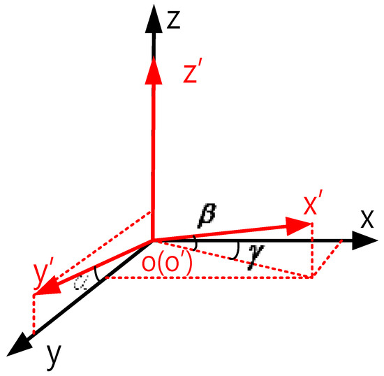
Figure 1.
Nonorthogonal schematic diagram of three-axis magnetic sensor.
Where refers to the angle between the axis and the axis, represents the angle between the axis and the plan, and stands for the angle between the projection of the axis in the plan and the axis. If only the nonorthogonal error is considered, then
where refers to the measured value of the three-axis magnetic sensor, represents the actual value of the three-axis magnetic sensor, and A stands for the nonorthogonal error matrix.
The magnetic core of the three-axis magnetic sensor is made of soft magnetic material with high permeability and low coercivity, which reaches its saturation state under external excitation that is then converted to the voltage value. After that, it collects the change in the measured magnetic field. The sensor contains detector circuit, integral filter circuit, and signal feedback circuit, etc. Different characteristics of electronic components in the circuit lead to differences in the sensitivity of the three axes. If only the sensitivity factor error is considered, then
where refers to the sensitivity factor of the axis, stands for the sensitivity factor of the axis, represents the sensitivity factor of the axis, and is the error matrix of the sensitivity factor.
Ideally, the sensor output should be zero in an absolutely zero magnetic field. However, the output is not zero because of the conversion zero drift of the signal processing circuit inside the sensor. If only this error is considered, then
where refers to zero drift.
Considering the above three errors, the error model of the three-axis magnetic sensor can be obtained as follows:
According to Equation (4), the comprehensive error calibration model of the three-axis magnetic sensor can be obtained as follows:
Replacing the by , and by , we can obtain:
Assumption , , where
The total magnetic field is invariable when the three-axis magnetic sensor changes its attitude in the uniform field. Therefore, the objective function can be expressed as
where refers to the predicted magnetic field with 9 unknowns, and represents the ideal magnetic field. The 9 unknowns are calculated by using the DA–LM algorithm. After that, the parameters of the nonorthogonal angle, scale factor, and zero bias are solved according to Equation (7). Finally, the error compensation process is completed.
3. Correction Algorithm
3.1. DA Algorithm
The DA algorithm is a bionics algorithm proposed in 2016 by Mirjalili, an Australian scholar [16].The main idea comes from the static foraging behavior and dynamic migration behavior of dragonflies in nature. In a static group, to search for other flying prey, the dragonflies made up of small parts fly back and forth over a small area. The local motion during flight and the temporary mutation in the flight path are the characteristics of static groups. In dynamic groups, for a better living environment, large groups of dragonflies fly long distances to migrate or fly in a common direction [19]. According to dragonfly behavior, the algorithm can be divided into: separation, queuing, alliance, hunting for prey, and avoiding natural enemies. The separation weight, alignment weight, cohesion weight, prey weight factor, and natural enemy weight factor in the algorithm are used as the behavior degrees of dragonflies to update their position. The algorithm can improve the initial random parameters of a given problem and make it converge to the global optimum [20].
The mathematical expression of the DA algorithm is expressed as follows:
where refers to the separation weight, represents the alignment weight, denotes cohesion weight, stands for the prey weight factor, is the natural enemy weight factor, refers to the current iteration number, represents the inertia weight, refers to the position vector of the separated behavior between the dragonfly, represents the position vector of the queuing behavior of the dragonfly, denotes the position vector of the alignment behavior of the dragonfly, represents the position vector of the hunting behavior of the dragonfly, and is the position vector of the avoidance behavior of the dragonfly.
In nature, dragonflies are in motion most of the time for survival. Therefore, their positions have to be updated in real time. Therefore, we obtain:
3.2. LM Algorithm
The LM is a modification of the Newton algorithm, which can be used to solve the problems that the Newton algorithm cannot guarantee, namely, that the search direction is always downward, and the Hessian matrix is always positively definite. The main idea of the Newton method is to use the first and second derivatives of iteration at Point to make a quadratic approximation to the objective function. Then, using the minimum point as the new iterative point, the process is repeated until the approximate minimum point satisfying the requirements of accuracy is obtained. When the objective function is second-order continuously differentiable, during the Taylor expansion of the function at point , the terms are ignored more than three times, and the quadratic approximation function can be obtained as follows:
where represents the first derivative of function at point , and stands for the second derivative of function at point . If the first-order necessary condition of the local minimum is applied here, then we obtain:
If , the minimum of function of is
which is the iterative formula of the Newton method. In case of univariate, if the second derivative of the function , the Newton method cannot converge to a minimum. While in case of multivariate, if the Hessian matrix of the objective function is not positively definite, the search direction determined by using the Newton method is not necessarily going to be the direction in which the value of the objective function decreases. To solve this problem, the damping coefficient is introduced, then the revised iteration formula is expressed as follows:
As long as is large enough, the search direction is ensured to be descending. Equation (14) is the iterative equation of the LM algorithm.
The goals and steps of the Algorithm 1: LM algorithm are as follows:
| Algorithm 1. LM algorithm. |
| and noisy can be estimated. and calculate . and construct incremental . from the incremental normal equations.
|
3.3. The Combination of DA and LM Algorithm
In solving the error parameters, we found that the number of least squares solutions were limited, while the LM algorithm can be used to solve multiple parameters simultaneously. However, the disadvantage of the LM algorithm is that it may fall into the local minima if the initial value is not appropriately selected, which has a serious impact on the accuracy of problem solving. To overcome this drawback, we used a global optimization algorithm to find the suitable initial value for the LM algorithm. As a global optimization algorithm, the DA algorithmhas the advantages of its strong global optimization ability. However, it has low accuracy in local optimization. To tackle this problem, this paper proposes to combine the DA algorithm and the LM algorithm. Firstly, this paper usedthe DA algorithm’s global optimization ability to find the global minimum point. Then, it took the output parameter value of the DA algorithm as the initial value of the LM algorithm for local optimization. The Figure 2 shows the flow chart of DA–LM algorithm.
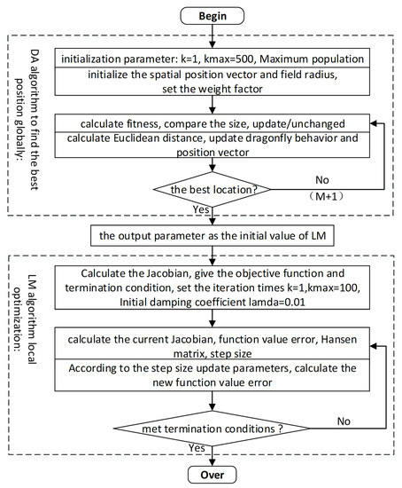
Figure 2.
The flow chart of DA–LM algorithm.
4. Simulated Analysis
Matlab is used for data simulation to verify the correctness and effectiveness of the proposed method based on the DA–LM algorithm in this paper. In the simulation analysis, the total magnetic field was set as 50,000 nT. Using the random function of Matlab to generate 96 groups of different angles, the rotation of the sensor was simulated, and then, the 96 groups of the ideal three-axis sensor rotation data H were obtained. The measured value was simulated by using Equation (4). The error parameter of the three-axis sensor is shown by the preset value in Table 1. The H1 three components of the magnetic field and the H1 total magnetic field are shown in Figure 3. The abscissa axis indicates the sampling points. The ordinate axes of (a), (b), and (c) indicate the components of the measured values H1 in x, y, and z, and the vertical axis of (d) represents the total magnetic field of the measurement H1. In addition, the red line refers to the ideal total magnetic field.

Table 1.
Comparison of preset and estimate parameters.
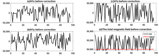
Figure 3.
The components and total magnetic field of H1 before correction. (a) The component of the measured values of x-axis; (b) The component of the measured values of y-axis; (c) The component of the measured values of z-axis; (d) The total magnetic field of measured values and ideal values.
By substituting, the ideal magnetic field and H1 into the objective function (Equation (8)) and using the LM and DA–LM respectively, the comprehensive parameters P and Q were solved. According to the relations among P, Q and the error parameters of the three-axis magnetic sensor, the error parameters were inversely solved. Table 1 shows the comparison between the error parameters obtained by inverse solution and the preset values. Finally, the magnetic field was corrected. The errors of the components and total magnetic field before and after correction are shown in Figure 4 where the abscissa axis represents the sampling point, and the ordinate axes of (a), (b), (c), and (d) stand for the errors of the x-axis, y-axis, z-axis, and the total magnetic field, respectively. The black lines show the errors before correction. And the blue lines represent the errors after correction.
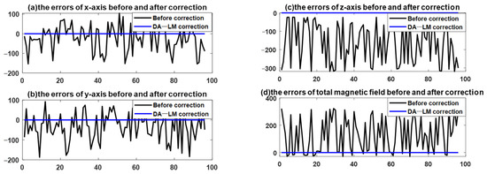
Figure 4.
The errors of components and total magnetic field before and after correction. (a) The errors of the x-axis; (b) The errors of the y-axis; (c) The errors of the z-axis; (d) The errors of measured total magnetic field before and after correction.
Seen from Figure 4, the errors of the x-axis, y-axis, z-axis, and the total magnetic field between the measured and ideal values are 200 nT, 200 nT, 350 nT, and 350 nT, respectively. After the DA–LM algorithm correction, all the errors were reduced to 0 nT.The parameter estimates are shown in Table 1.
It can be seen from the comparison among the preset parameter values, LM estimate values, and DA–LM estimate values in Table 1 that the LM algorithm alone cannot accurately estimate the error parameters, especially when the nonorthogonal angle is very small. The reason is that the initial value is given empirically when the LM algorithm is used alone. If the initial value is given improperly, the minima will be trapped in the local minimum. The error parameters calculated by using the DA–LM algorithm were almost the same as the preset value, with the error accuracy of estimation of 10−6 magnitude. The simulation results show that the global optimization ability of the DA algorithm can help the LM algorithm find the most suitable initial value and effectively prevent the LM algorithm from falling into the local minimum.
5. Experimental Verification
In addition to its own error, the sensor is also susceptible to many factors, for instance, magnetic diurnal variation. To mitigate the influence of the magnetic diurnal variation on the magnetic field, experiments were carried out after 12 p.m. The ideal total magnetic field H was measured by using an optical pump magnetometer with high precision, as shown in Figure 5. The actual measurement value H1 was obtained by using the three-axis magnetometer MAG648. The experiment platform is as shown in Figure 6. In Figure 7, the abscissa axis represents the sampling point of the measured data, and the ordinate axis stands for the total value of the magnetic field. The red line refers to the ideal total magnetic field modulus, while the black line shows the measurement total magnetic field H1 before correction. The blue line refers to the total magnetic field after LM correction, and the green line denotes the total magnetic field after DA–LM correction. It is obvious that the DA–LM correction effect outperforms that of LM correction.
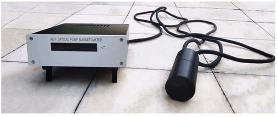
Figure 5.
The optical pump magnetometer with high precision.
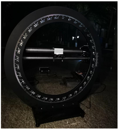
Figure 6.
The experiment platform with the three-axis magnetometer MAG648.
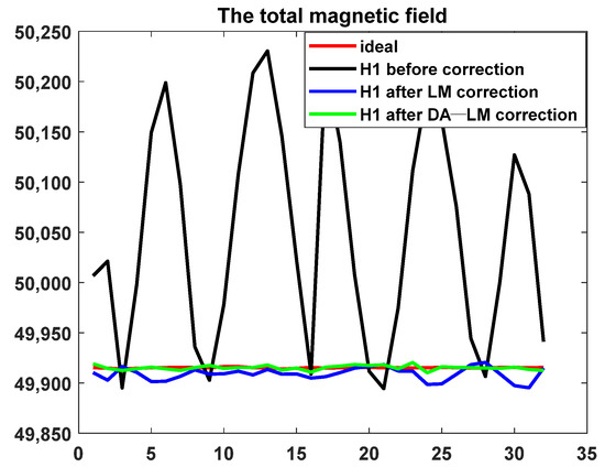
Figure 7.
The total magnetic field before and after correction.
In Figure 8, the abscissa axis refers to the sampling point, and the ordinate axis represents the error between the total value measured data and the ideal total value. In addition, the value is reduced from 300 nT to 5 nT and 20 nT after DA–LM and LM correction, respectively. We drew a conclusion that the steering error was significantly suppressed. The parameters shown in Table 2 were solved by using the DA–LM method and LM method, respectively. Table 3 shows the comparison between the mean value and the root mean square error. It can be seen from the Table that the mean value and root mean square error were reduced after DA–LM correction.
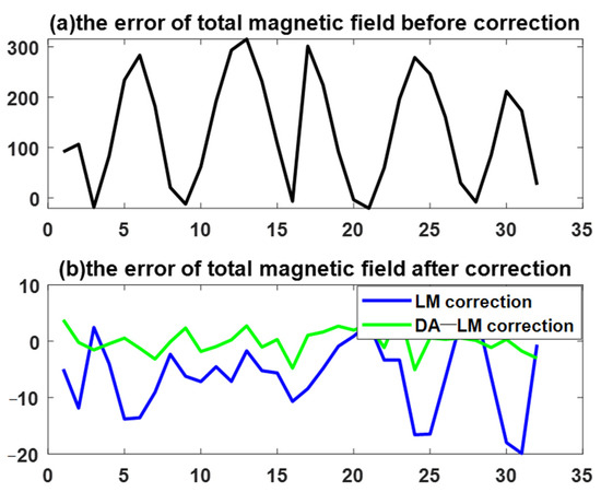
Figure 8.
The error of total magnetic field before and after correction. (a) The error of total magnetic field before correction; (b) The error of total magnetic field after correction, and the blue line represents the LM correction, the green line represents the DA–LM correction.
Table 2.
The parameters obtained by calculation.
Table 3.
Comparison of statistical characteristics before and after DA–LM correction.
6. Conclusions
Geomagnetic error correction is the key to obtaining high-precision geomagnetic information and the premise of magnetic anomaly location. Error correction has always been the focus of research on magnetic measurement, and many correction algorithms have been proposed under different application backgrounds. This paper analyzed the error sources of magnetic sensors, proposed a method combing the DA algorithm and the LM algorithm to iteratively solve the parameters in the error model, and finally completed the error compensation. The following conclusions are drawn: (1) The method combining the DA and LM algorithms can accurately calculate the error parameters, which solves the problem that it may easily fall into the local minimum in the iterative process by using the LM algorithm alone; (2) The simulation results show that the proposed method can accurately estimate the error parameters and has a good correction effect on the components and total magnetic field, thereby proving the effectiveness of the proposed algorithm. It can be seen from the experimental results that this method can estimate the error parameters of sensors well, with the RMS value reduced from −131.807381 nT/m to 0.000247 nT/m and the RMSE value from 109.523401 nT/m to 2.285982 nT/m. The experimental data were only calibrated for the total magnetic field due to the unavailability of the ideal three-component values with high accuracy. In the event the ideal three-component can be obtained, this method can also be applied to three-component correction.
Author Contributions
Conceptualization, C.L. and L.Y.; methodology, C.L. and L.Y.; software, C.L., L.Y. and S.Z.; validation, C.L. and L.Y.; investigation, C.L., L.Y., S.Z., S.X., X.T. and Y.L.; data curation, H.C., S.Z. and C.X.; writing–original draft preparation, C.L.; writing–review and editing, C.L. and L.Y.; supervision, L.Y., C.X. and H.C. All authors have read and agreed to the published version of the manuscript.
Funding
This research received no external funding.
Institutional Review Board Statement
Not applicable.
Informed Consent Statement
Not applicable.
Data Availability Statement
All of the data in our paper are not publicly archived data.
Conflicts of Interest
The authors declare no conflict of interest.
References
- Sun, X.J.; Kou, J.; Zhang, X.N.; Li, J. Research Progress in Geomagnetic Navigation. Navig. Control 2016, 15, 1–6. [Google Scholar]
- Pan, Q.J.; Ma, W.M.; Zhao, Z.H.; Kang, J. Development and Application of Measurement Method for Magnetic Field. Trans. China Electrotech. Soc. 2005, 7–13. [Google Scholar] [CrossRef]
- Ma, J.Y. Application of high precision magnetic prospecting in regional investigation. World Nonferr. Met. 2018, 33, 148–149. [Google Scholar]
- Bilukha, O.O.; Brennan, M.; Anderson, M. Injuries and Deaths From Landmines and Unexploded Ordnance in Afghanistan 2002–2006. JAMA 2007, 298, 516–518. [Google Scholar] [CrossRef] [PubMed] [Green Version]
- Pei, Y.L.; Liu, B.H.; Zhang, G.E.; Liang, R.C.; Li, X.S. Application of Magnetic Method to Ocean Engineering. Adv. Mar. Sci. 2005, 114–119. [Google Scholar]
- Song, H.; Zou, L.; Zhang, X.Q.; Zhang, L.; Zhao, T. Inter-Turn Short-Circuit Detection of Dry-Type Air-Core Reactor Based on Spatial Magnetic Field Distribution. Trans. China Electrotech. Soc. 2019, 34 (Suppl. 1), 105–117. [Google Scholar]
- Pham, D.M.; Aziz, S.M. A real-time localization system for an endoscopic capsule using magnetic sensors. Sensors 2014, 14, 20910–20929. [Google Scholar] [CrossRef] [PubMed] [Green Version]
- Shi, G.; Li, X.S.; Li, X.F.; Liu, Y.X.; Kang, R.Q.; Shu, X.Y. Equivalent two-step algorithm for the calibration of three-axis magnetic sensor in heading measurement system. Chin. J. Sci. Instrum. 2017, 38, 402–407. [Google Scholar]
- Liu, J.J.; Chen, L.; Wang, D.J.; Qi, H.X. Correction method of 3-axis magnetic sensor. Mod. Electron. Tech. 2018, 41, 179–181+186. [Google Scholar]
- Li, X.; Li, Z. Dot product invariance method for the calibration of three-axis magnetometer in attitude and heading reference system. Chin. J. Sci. Instrum. 2012, 33, 1813–1818. [Google Scholar]
- Li, X.; Song, B.Q.; Wang, Y.J.; Niu, J.H.; Li, Z. Calibration and Alignment of Tri-Axial Magnetometers for Attitude Determination. IEEE Sens. J. 2018, 7399–7406. [Google Scholar] [CrossRef]
- Luo, J.G.; Li, H.B.; Liu, J.X.; Li, H.H.; Zhang, F. Study on Error Correction Method of Three-axis Fluxgate Magnetometer. Navig. Control 2019, 18, 52–58. [Google Scholar]
- Pang, H.F.; Luo, S.T.; Chen, D.X.; Pan, M.C.; Zhang, Q. Error Calibration of Fluxgate Magnetometers in Arbitrary Attitude Situation. J. Test Meas. Technol. 2011, 25, 371–375. [Google Scholar]
- Wang, Q.B.; Zhang, X.M. Research of fast calibration method of three-axis magnetic sensor. China Meas. Test 2017, 43, 35–39. [Google Scholar]
- Pang, X.L.; Lin, C.S. Calibration Coefficients Solving of Three-Axis Magnetic Sensor Based on Genetic Algorithm. J. Detect. Control 2017, 39, 42–45+51. [Google Scholar]
- Mirjalili, S. Dragonfly algorithm: A new meta-heuristic optimization technique for solving single-objective, discrete, and multi-objective problems. Neural. Comput. Appl. 2016, 27, 1053–1073. [Google Scholar] [CrossRef]
- Zhang, H.Y.; Geng, Z. Novel interpretation for Levenberg -Marquardt algorithm. Comput. Eng. Appl. 2009, 45, 5–8. [Google Scholar]
- Zhang, J.; Chen, J.; Yang, S.H. The Study of Calibration Method of Magnetic Resistance Sensor. J. Proj. Rocket. Missiles Guid. 2010, 30, 46–48. [Google Scholar]
- Wu, W.M.; Wu, W.Y.; Lin, Z.Y.; Li, Z.X.; Fang, D.Y. Dragonfly algorithm based on enhancing exchange of individuals’ information. Comput. Eng. Appl. 2017, 53, 10–14. [Google Scholar]
- Qiao, M.Y.; Xu, C.K.; Tang, X.X.; Gao, Y.F.; Shi, J.K. Application Research of DA-LM Algorithm in Error Correction of MEMS Accelerometer. Chin. J. Sens. Actuators 2021, 34, 223–231. [Google Scholar]
Publisher’s Note: MDPI stays neutral with regard to jurisdictional claims in published maps and institutional affiliations. |
© 2022 by the authors. Licensee MDPI, Basel, Switzerland. This article is an open access article distributed under the terms and conditions of the Creative Commons Attribution (CC BY) license (https://creativecommons.org/licenses/by/4.0/).