Mathematical Modeling of Multi-Performance Metrics and Process Parameter Optimization in Laser Powder Bed Fusion

Abstract

This study aims to develop mathematical models to improve multi-performance metrics, such as relative density and operating costs, in laser powder bed fusion (LPBF), also known as selective laser melting, a metallic additive manufacturing technique, by optimizing the printing process parameters. The work develops a data-driven model for relative density based on measurements and an analytical model for operating costs related to the process parameters. Optimization models are formulated to maximize relative density or minimize operating costs by determining the optimal set of process parameters, while meeting a target level of the other performance metrics (i.e., relative density or operating costs). Furthermore, new metrics are devised to test the sensitivity of the optimization solutions, which are used in a novel robust optimization model to acquire less sensitive process parameters. The sensitivity analysis examines the effect of varying some parameters on the relative density of the fabricated specimens. Samples with a relative density greater than 99% and a machine operating cost of USD 1.00 per sample can be produced, utilizing a combination of low laser power (100 W), high scan speed (444 mm/s), moderate layer thickness (0.11 mm), and large hatch distance (0.4 mm). This is the first work to investigate the relationship between the quality of the fabricated samples and operating cost in the LPBF process. The formulated robust optimization model achieved less sensitive parameter values that may be more suitable for real operations. The equations used in the models are verified via 10-fold cross-validation, and the predicted results are further verified by comparing them with the experimental data in the literature. The multi-performance optimization models and framework presented in this study can pave the way for other additive manufacturing techniques and material grades for successful industrial-level implementation.

1. Introduction

In the last decade, additive manufacturing (AM) has seen tremendous growth in various sectors, including healthcare, automotive, electronics, and aerospace. AM has shown greater flexibility than conventional techniques for the manufacture of small-volume, complicated, and customized components [1]. The laser powder bed fusion (LPBF) process, also commonly referred to as selective laser melting (SLM), is the most common metal AM technique, in which layers of metallic powder are selectively melted using a high-power laser beam and nearly fully dense sections are fabricated for each layer [2]. However, despite the popularity of LPBF, its application in industry is currently limited, due to inherent process characteristics associated with high cost in correlation to the process parameters [3,4,5].

For most of the functional applications of LPBF-produced parts, dimensional accuracy, surface roughness, relative density (RD), and strength of the parts are considered important properties [6]. In addition to this, the associated operational cost plays a key role from an economic point of view. While a higher RD of parts fabricated by the LPBF process is preferred or required in some industries (e.g., the aerospace industry), it may incur a higher manufacturing cost due to higher operating costs, associated with longer processing times or increased energy consumption. Therefore, optimizing process parameters is critical for process planning, maintaining acceptable finished part quality, as well as reducing operational costs in order to increase the commercial adoption of the technology. Extensive research is available on AM process optimization to produce metal parts with the desired quality and properties.

Researchers have made several attempts to improve the performance of the AM parts through the formulation of statistical models followed by optimization techniques [7]. Some of the statistical models used in the literature were the Taguchi method [8], response surface methodology [9], regression analysis, and design of experiment [10]. Because AM systems are non-linear and complex, powerful optimization techniques were used to identify optimal parameter values for better-manufactured part quality. Some of the optimization algorithms used in the literature were the Genetic Algorithm (GA) [11] and swarm intelligence algorithm [12]. Major research work has been conducted in the area of optimization of process parameters for different metal AM processes. The most important optimization approaches can be grouped into two main categories: single-objective optimization and multi-objective optimization.

Many researchers utilized a single-objective optimization approach by investigating the effects of certain important process parameters on a single property of the fabricated parts (i.e., RD). Read et al. [13] studied the influence of LPBF parameters on the porosity fraction of fabricated AlSi10Mg by utilizing a statistical experimental design. Their results suggested using high laser power, low scan speed, and small hatch spacing to minimize the porosity content within the material. Laakso et al. [14] followed an optimization approach based on finite element analysis to study the influence of process parameters, such as laser power, scan speed, and hatch width on the RD of tool steel H13 parts. An optimal parameter window was suggested, and steel parts with high RD were fabricated by LPBF. Similarly, Aboutaleb et al. [15] proposed an accelerated process optimization methodology and investigated the effect of laser power, laser velocity, hatch distance, and layer thickness on the RD of 17-4 PH stainless-steel parts fabricated by LPBF. Their proposed methodology obtained a combination of optimal process parameters with fewer experimental trials, resulting in an average part density of 99.2%. Moreover, a similar investigation about the effect of laser power, scan speed, and hatch distance on the RD of AlSiMg0.75 aluminum alloy and Cu-15Sn copper alloy was conducted by Bai et al. [16] and Mao et al. [17], respectively, using the design of experiment-based optimization. Nearly fully dense specimens (>99%) were fabricated utilizing the optimal processing parameter set in both studies. AlFaify et al. [9] used the response surface method to obtain optimal parameter combinations for high-density stainless-steel 316L (SS316L) parts. Sample RD of approximately 99% was attained at a point distance = 0.07 mm, exposure time = 0.12 ms, hatching distance = 0.12 mm, and layer thickness = 0.05 mm. Another study, by Yakout et al. [18], obtained an optimum process window for laser process parameters and dense components from Invar 36 and SS316L with RD greater than 97% were fabricated. More recently, Vallejo et al. [19] provided a comprehensive understanding of the effects of laser power, scan speed, and hatch spacing on the densification behavior of SS316L. Samples with RD greater than 99.8% were fabricated at a power = 200 W, scan speed = 800 mm/s, hatch spacing = 0.12 mm, and layer thickness = 0.03 mm.

In addition to the RD, other part characteristics were investigated using the single-optimization approach by several researchers. The relationship between the surface roughness and input processing parameters of AlSiMg0.75 aluminum alloy parts fabricated by LPBF was studied by Majeed et al. [20]. Their study utilized a design of experiment approach and obtained the lowest surface roughness of 3.35 µm at 400 W laser power, 600 mm/s of scan speed, and 0.25 overlap rate. Using the same approach, Samantaray et al. [21] found the optimal process parameters, including laser power, scan speed, porosity percentage, laser spot size, and powder bed thickness, which resulted in a maximum sintering depth of 3 mm for AlSiMg0.75 aluminum alloy parts produced by the direct metal laser sintering process.

Multi-objective optimization has also been used to improve multiple characteristics in different metallic alloys fabricated by LPBF. Arısoy et al. [22] investigated the optimization of microstructural properties, including grain size and growth directions, for IN625 nickel alloy parts based on laser power, scan velocity, hatch distance, and scan strategy. Process parameters that resulted in the optimum responses with trade-offs were identified. Shi et al. [23] experimentally analyzed the effect of laser power and scan speed on the building rate and RD of Ti-6Al-4V titanium alloy parts. Using the optimized process parameters, a high RD of 99.99% was observed and a maximum building rate of 9 mm³ was reached.

Maamoun et al. [24] utilized a design of experiment to obtain the optimal settings of laser power, scanning speed, and hatch spacing. Their study achieved high-quality AlSi10Mg and Al6061 parts, in terms of RD, porosity, surface roughness, and dimensional accuracy. Mutua et al. [25] identified the optimal combination of laser power, scan speed, and spot diameter that affected the RD and surface quality of maraging steel. The optimum process conditions resulted in a maximum RD of 99.8% and good surface quality, with a roughness value of 35 μm. A study by Aboutaleb et al. [26] proposed a multi-objective accelerated process optimization approach utilizing data from previous studies and obtained the highest RD of 98.39% and elongation to failure of 2.22% for Ti-6Al-4V parts.

Other studies applied a multi-objective optimization approach for the LPBF process to fabricate SS316L parts. Wang et al. [27] determined the optimal process settings of speed function and focus offset that resulted in high RD (99%) and well-melted top-build surface SS316L parts, fabricated by electron beam melting. Deng et al. [28] and Sun et al. [29] used different experimental techniques to optimize process parameters and obtain the desired mechanical properties for SS316L parts. They produced high-quality parts in terms of tensile strength, density, and surface roughness that can further improve the fatigue properties of the material. Similarly, Pant et al. [30] followed a design of experiment approach and developed an optimization model for SS316L parts produced by direct metal laser sintering. The model resulted in the optimal settings of laser power, scan speed, and powder flow rate that achieved a catchment efficiency of 40.72% and clad height of 0.667 mm. Recently, a US patent by Bonakdar et al. [31] presented a statistical and experimental methodology for optimizing target output material properties in an AM process.

The aforementioned studies confirm that the optimization of AM process parameters is an essential task for obtaining high-quality parts with superior properties [32]. However, the biased nature of the single-objective optimization approach and the complexity of multi-objective optimization may pose a challenge in efficiently utilizing these approaches. Therefore, there is a need to develop an efficient optimization approach that reduces these limitations. To the best of our knowledge, no prior research has addressed both the RD and operating cost of samples fabricated by LPBF. Here, we raise a few important questions that prior studies could not address adequately. What is the most effective way to optimize LPBF process parameters? How can we model the important metrics mathematically for engineering methods?

To address these questions, this study aims at developing mathematical models to optimize the LPBF process parameters concerning the RD of SS316L stainless-steel samples and the operating cost of the LPBF process. To achieve this goal, this study sets the first research objective as the development of a data-driven model for RD and an analytical model for operating costs, using several components related to the LPBF process parameters. The second objective is to develop optimization models to obtain the optimal set of process parameters, namely, laser power, scan speed, hatch distance, and layer thickness, considering different performance metrics, such as RD and operating costs, and, thereby, achieve a rational trade-off between the RD and operating cost. The central hypothesis in this study is that the formulation and solution for such a multi-performance metric optimization problem can provide optimal process parameters, which can render samples with high RD at an acceptable operating cost, without the need to perform extensive experimental trials. In addition, the present study examines a method to acquire less sensitive process parameters and conducts a sensitivity analysis to understand the effect of varying some model input parameters on the RD of the samples.

The rest of the paper is organized as follows. Section 2 describes the methods and Section 3 provides and discusses the basic results. Section 4 presents a robust optimization model, extended from the model in Section 2. Then, Section 5 additionally conducts sensitivity analysis by considering different fabrication scenarios. Lastly, Section 6 draws conclusions.

2. Methods

Figure 1 illustrates the overall process of the methods used in this study to evaluate the model and optimize the process parameters of SS316L samples fabricated by LPBF. The stainless-steel-grade SS316L is widely used in metal AM processes. The alloy is considered a desirable industrial material because of its outstanding corrosion resistance, good weldability, high strength, and relatively low cost [27]. In the first stage of this study, an extensive dataset is created by systematically combining experimental results from prior studies, including our recent work [33]. In the data modeling stage, the collected data are split for training and testing processes and a regression model is developed based on the training data. Then, cross-validation is applied to check the data model accuracy according to the mean square error (MSE) and coefficient of determination (R²). Finally, in the optimization stage, a multi-performance metric optimization model is formulated using the obtained regression model and a developed cost model for the LPBF process. Based on the optimization model, a novel robust optimization model is further formulated to acquire less sensitive process parameters. The GA solves the optimization models to determine the optimal process parameters. The following sensitivity analysis examines the variation in the quality of the samples with respect to the model input parameter change.

2.1. Data Collection

The experimental data used in this study were extracted from different studies related to the RD of SS316L samples fabricated by LPBF, as presented in

Table 1. Studies from the literature used for data collection.

No.	Reference	#Data	Machine	Mean RD
1	[34]	43	Concept Laser GmbH M2	97.67%
2	[35]	31	Concept Laser GmbH M1	98.08%
3	[36]	13	Concept Laser GmbH Mlab-Cusing	94.56%
4	[37]	44	Concept Laser GmbH Mlab-Cusing	86.06%
5	[38]	9	EOS GmbH M290	99.79%
6	[39]	6	SLM Solutions GmbH	95.77%
7	[40]	10	SLM Solutions GmbH 280HL	98.59%
8	[41]	3	Renishaw AM250	97.97%
9	[42]	9	Renishaw AM250	96.23%
10	[9]	24	Renishaw AM250	97.53%
11	[23]	4	Renishaw AM400	99.87%
12	[43]	32	Laseradd DiMetal-100	93.90%
13	[33]	20	EOS M400-4	98.60%

. The studies contain different numbers of observations representing the experimental parameters and the measured RD of SS316L samples fabricated by different LPBF machines. The last column provides the mean RD of each study.

The compiled dataset contains 248 observations. Data cleansing started with the detection of potential outliers by observing the standardized residuals of least-squares regression. An observation with a standardized residual greater than 3 (in absolute value) is considered to be an outlier [44]. The outlier-removal process reduced the size of the final dataset to 197 observations.

2.2. Relative Density (RD) Data Modeling

A significant number of parameters can affect the quality of LPBF parts, where laser power, scan speed, hatch distance, and layer thickness are most commonly investigated in the literature. One of the major challenges in manufacturing metallic parts for final applications is accurately predicting the characteristics of the fabricated parts due to the non-linear and complex nature of the process [32]. Regression analysis is employed to build a mathematical relationship between the RD and process parameters. Polynomial regression is a special case of multiple linear regression where a curvilinear relationship is established between the dependent and independent variables. Interactions between different combinations of variables can be taken into account by including interaction terms in the polynomial model. Several studies in the literature utilized second-order multivariable polynomial regression to establish a relationship model between the process parameters and part quality of SS316L parts fabricated by LPBF [18,30,45].

Polynomial regression has been widely used in data modeling, especially for AM processes. Moreover, a closed-form mathematical expression is highly preferred to formulate an optimization model (see Section 3). Thus, the present study develops a second-order multivariable polynomial regression model with interaction terms to predict the RD of SS316L samples fabricated by LPBF. The RD of the fabricated samples is modeled as a function of the selected process parameters (i.e., laser power, scan speed, hatch distance, and layer thickness). Using MATLAB R2021a software, a second-order multivariable polynomial model was obtained:

$$\begin{gathered} RD\left(p, v, h, t\right)=82.688+0.13659 p-0.0030294 v+122.93 h-169.9 t+0.000075901 pv+0.67386 ph+ \\ 1.4043 pt-0.012368 vh-0.16949 vt+500.94 ht-0.00038539 p^2-0.0000039611 v^2-9.2705 h^2 \\ -1050 t^2, \end{gathered}$$

(1)

where RD (p, v, h, t) is RD, p is laser power in W, v is scan speed in mm/s, h is hatch distance in mm, and t is layer thickness in mm. The polynomial model for the RD involves terms with the independent variables (p, v, h, t), quadratic variables (p², v², h², t²), and two-way interactions (pv, ph, pt, vh, vt, ht).

In order to judge the adequacy of the fitted regression model, k-fold cross-validation is used to compare the predicted and observed values of RD. The fold number k is often chosen to be 5 or 10 and represents the number of parts into which the data are divided; k-1 folds for training and the remaining fold is used for testing the model [46,47]. The accuracy of the model is evaluated using the average MSE and R² from 10 folds, and the developed model appears to fit the data well with R² of 82.49% and MSE of 4.216. Considering other machine learning algorithms tested for a similar system by Abdulla et al. [33] and Barrionuevo et al. [46], the developed model showed a sufficiently high R² value. Thus, the model may be suitable for predicting the RD of SS316L samples fabricated by LPBF. It is worth noting that excluding the small coefficient terms (i.e., $p^2$ and $v^2$) was not helpful in improving R² and MSE.

2.3. Cost Modeling

Due to the commercial impacts of the high production cost of AM, several researchers have placed a strong emphasis on cost estimation and reduction for AM techniques [48,49,50,51]. The production cost of AM-built parts can be broken down into costs for machine operation, labor, and material. Labor cost is determined by the interaction of labor forces, including the costs of setting up the machine, operating software, maintenance, preprocessing, and postprocessing [52]. Material cost depends on the mass and price of raw materials used in production. Machine operating cost is one of the most significant costs involved in AM. Most of the cost models established in the literature are based on assumed fixed process parameters. However, the appropriate selection of process parameters can help save production time, reduce costs, and improve overall productivity.

In LPBF, laser beams selectively melt powder layers while ensuring complete melting along the scan track, allowing fusion to occur between tracks and successive layers, and resulting in dense parts with good mechanical performance [53]. This study presents cost models based on the specifications of the EOS M 400 machine. Figure 2 illustrates the sample layout in the chamber of the LPBF system under consideration. Samples are divided into a number of layers based on the layer thickness, and a rotating roller evenly distributes the metal powder across the substrate plate. Then, selected areas in the layer are melted and fused with a high-power laser. After completing the scan of one layer, the substrate moves down by a certain distance equal to the layer thickness and a new layer of powder is deposited. The layer-by-layer process repeats until the samples are completed [54].

The build length of the EOS M 400 machine is 400 mm [55]. It is assumed that cubic SS316L samples with 10 mm per side are fabricated with a distance of 2.5 mm between each sample in the build platform.

Machine operating cost is controllable by adjusting process parameters, while labor and material costs are not directly related to the process parameters. Thus, the scope of the cost analysis in this study focuses only on the machine operating cost. If needed, the total production cost can be calculated by the sum of the resultant operating cost with the material and labor costs that need further analysis for a selected manufacturing scenario. In addition, even though the LPBF process is usually utilized for the batch production of parts, analysis of the operating cost in this study is only based on a single-specimen configuration. Hence, the machine operating cost ($C_o$) is estimated based on two main components, fabrication cost per sample ($C_f$) and energy cost per sample ($C_e$), via

$$C_o=C_f+C_e$$

(2)

The fabrication cost $C_f$ is mainly related to the operation rate of the AM machine and is calculated by multiplying the fabrication time ($T_f$) in seconds by the machine’s hourly operating cost ($C_{mc}$):

$$C_f=T_f\times \frac{C_{mc}}{3600}$$

(3)

In the LPBF process, the fabrication time is the sum of scanning time ($T_s$) and recoating time ($T_r$):

$$T_f=T_s+T_r$$

(4)

The laser is controlled by a scanning device that selectively melts the sample cross-section for each iteration. The scanning time can be calculated by dividing the sample volume ($V$) in mm³ by the build rate. The build rate is determined by the product of the scan speed, hatch distance, and layer thickness. Thus, the scanning time is given by

$$T_s=\frac{V}{v\times h\times t}$$

(5)

On the other hand, the recoating time is related to the recoating process, which lays or deposits material on each layer for further processing [56]. The recoating time is calculated by the product of the number of layers and recoating time per layer ($T_L$) in seconds. The number of layers for a sample can be computed by dividing the sample height ($H$) in mm by layer thickness. The recoating time is

$$T_r=\frac{H}{t}\times T_L$$

(6)

From the above equations, the fabrication cost in Equation (3) can be re-written as

$$C_f=\left(T_s+T_r\right)\times \frac{C_{mc}}{3600}=\left(\frac{V}{v\times h\times t}+\frac{H}{t}\times T_L\right)\times \frac{C_{mc}}{3600}$$

(7)

In Equation (7), the machine’s hourly operating cost ($C_{mc}$) is divided by 3600 to make all time units consistently in seconds.

Metal AM is an energy-intensive process as it utilizes a laser beam or electron beam with high power density to melt materials fully. The energy consumption of metal AM processes can be defined in several ways. Energy consumption at the machine level refers to the energy consumed by the subsystems of the machine and in various operational modes. On the other hand, energy consumption at the process level is related to the energy flow distribution in an AM system. This requires understanding the system’s thermal history and dynamic behavior [56].

The energy consumption in this study is estimated based on the machine level to provide a generic model that can be utilized in different LPBF processes. The energy consumption cost is calculated as the product of the fabrication time (as defined in Equation (4)), machine power consumption ($E_{mc}$) in kW, and electricity rate ($C_{\mathrm{electricity}}$) in USD /kWh:

$$C_e=\left(\frac{V}{v\times h\times t}+\frac{H}{t}\times T_L\right)\times E_{mc}\times \frac{C_{\mathrm{electricity}}}{3600}$$

(8)

It is worth noting here that an environmental impact related to energy consumption can be easily considered by adding an environmental cost to the electricity rate [57]. Finally, the machine operating cost ($C_o$) in Equation (2) can be re-written as

$$C_o\left(v, h, t\right)=\left(\frac{V}{v\times h\times t}+\frac{H}{t}\times T_L\times \frac{C_{mc}}{3600}\right)+\left(\frac{V}{v\times h\times t}+\frac{H}{t}\times T_L\right)\times E_{mc}\times \frac{C_{\mathrm{electricity}}}{3600}$$

(9)

Equation (9) illustrates the generic model constructed for estimating the machine operating cost of a sample based on the fabrication and energy costs. Several processing parameters have an impact on both the operating cost and the RD of the sample. Therefore, the process parameters should be adjusted carefully to obtain high-quality samples with acceptable operating costs. The cost model contains several assumptions and constants, and

Table 2. Cost model parameters.

Model Parameters	Value	Unit
Sample Volume (V)	1000	mm3
Sample Height (H)	10	mm
Recoating time per layer ($T_L$)	0.375	s
Machine’s hourly operating cost ($C_{mc}$)	40	USD /h
Machine power consumption ($E_{mc}$)	16.2	kW
Electricity rate ($C_{\mathrm{electricity}}$)	0.1376	USD /kWh

presents the model parameters used in this study.

The cost model parameters are user defined and can be changed depending on the required dimensions of the fabricated samples, type of machine used, and country of fabrication. The cost model in this study is based on the fabrication of cube samples with 10 mm sides, as illustrated in Figure 2. The geometry of the sample is assumed to be cubic to avoid any additional costs, such as cleaning (in the case of hollow samples) or removal of support structures. The recoating time per layer for a single sample was estimated to be 0.375 s based on the specifications of the EOS M 400 and the assumption that the recoating procedure takes roughly 12 s [58].

The machine’s hourly operating cost is assumed to be USD 40/h, as the typical hourly operation costs of metal AM machines can range from about USD 37/h to USD 90/h [59]. The machine power consumption is obtained from the specifications of the EOS M 400, with the typical power consumption of the machine being 16.2 kW within a normal range of the operating laser power [55]. The electricity rate depends on the region of fabrication and differs from one country to another. The value of the electricity rate selected for the cost model is related to the average commercial electricity rate in the U.S. obtained from ChooseEnergy.com (accessed on 13 September 2021), which is USD 0.1376/kWh [60].

2.4. Optimization Modeling

This section formulates two optimization models utilizing the defined metrics (i.e., the RD in Equation (1) and the operating cost per sample in Equation (9)). Since each of the presented models handles two important performance metrics, we name them multi-performance metric optimization models. The decision variables in the optimization models are the parameters of the LPBF process, including laser power (p), scan speed (v), hatch distance (h), and layer thickness (t). The lower and upper bounds for the process parameters are presented in

Table 3. Process parameters and their levels in the optimization models.

Decision Variable	Description	Unit	Lower Limit	Upper Limit
p	Laser power	W	100	400
v	Scan speed	mm/s	200	2500
h	Hatch distance	mm	0.10	0.4
t	Layer thickness	mm	0.02	0.25

. The process parameters affect the RD and the machine operating cost of the sample simultaneously. Thus, it is important to determine the optimal set of process parameters that achieves the highest RD of a sample with a lower operating cost.

(1)

Maximization of relative density

The first optimization model (Model 1) aims at maximizing the RD while maintaining the machine operating cost ($C_o$) within a limit. The objective, Equation (10), is to maximize the RD, which is a function of process parameters. The constraint given by Equation (11) restricts the total machine operating cost to be within the cost limit ($C_1$). Constraints (12–15) maintain the process parameters within their lower and upper limits, which were determined based on the min and max values in the dataset used.

Model 1:

$$Max.RD\left(p, v, h, t\right)$$

(10)

subject to

$$C_o\left(v, h, t\right)\le C_1,$$

(11)

$$200 \le v \le 2500,$$

(12)

$$100 \le p \le 400,$$

(13)

$$0.10 \le h \le 0.4,$$

(14)

$$0.02 \le t \le 0.25.$$

(15)

(2)

Minimization of machine operating cost

The second optimization model (Model 2) aims to minimize the machine operating cost of a sample fabricated by LPBF while meeting the minimum RD. Model 2 includes the objective function (16) to minimize the machine operating cost ($C_o$) of a sample. Constraint (17) assures that the RD of the sample should be at least at the minimum bound ($C_2$).

Model 2:

$$Min. C_o\left(v, h, t\right)$$

(16)

subject to

$$RD\left(p, v, h, t\right)\ge C_2,$$

(17)

and Equations (12)–(15).

(3)

Solution method using GA

Since the formulated optimization models are non-linear, they are solved using the GA in MATLAB. GA is one of the most widely used meta-heuristics that solves non-linear or large-scale linear optimization problems by reflecting the process of natural evolution. The GA begins with a random population of a few individuals and progresses to better populations or groups of individuals. Sometimes, it allows a worse movement at some iterations randomly to handle the issue of entrapping in a local-optimum existing in a non-linear problem [61]. GA uses several operators to produce the next generation of the population, such as scaling, selection, crossover, and mutation [62]. By using different operators, the incumbent solution value may improve or worsen. Choosing a good set of GA parameters is usually obtained by trial and error in many heuristics approaches [63]. In this work, the default options of the GA in MATLAB are utilized. These include a population size of 50, crossover probability of 0.8, mutation probability of 0.1, and termination criteria represented by the maximum number of generations, which is fixed at 100.

3. Results and Discussion

Table 4. Optimization results of Model 1 for different cost bounds ($C_1$).

No.	Machine Operating Cost Bound C1 (USD)	RD (%)	p (W)	v (mm/s)	h (mm)	t (mm)
1 *	1.00	99.26	100	444	0.4	0.11
2	0.90	96.8	400	565	0.149	0.203
3	0.80	98.73	108	514	0.4	0.126
4	0.70	98.16	199	341	0.4	0.186
5	0.60	97.15	191	489	0.4	0.173
6	0.50	90.31	270	368	0.4	0.25
7	0.40	87.03	334	521	0.4	0.25
8	0.30	74.77	322	938	0.4	0.25
9	0.20	No solution	-	-	-	-

* Optimal process parameter set obtained from setting the cost limit (C₁) to USD 1.00 per sample.

provides the results of Model 1. Case 1* indicates the optimal process parameter set obtained from setting the cost limit ($C_1$) to USD 1.00 per sample as a basic cost. Samples with a maximum RD of 99.26% can be fabricated at a laser power of 100 W, scan speed of 444 mm/s, hatch distance of 0.4 mm, and layer thickness of 0.11 mm. The optimal solutions of the process parameters indicate that the highest RD can be achieved utilizing low laser power, high scan speed, moderate layer thickness, and large hatch distance.

The rest of the cases in Table 4 show the variation in the optimal RD with respect to different cost bounds ($C_1$ values) in Model 1 between USD 1.00 and USD 0.20. As $C_1$ decreases, the RD generally decreases until the algorithm cannot find any feasible combination of process parameters at USD 0.20 per sample. The machine operating cost per sample ($C_o$), which is restricted by $C_1$ in constraint (11) of Model 1, is a function of the process parameters. Thus, high bounds for the cost provide more room for improvement in the RD, as the algorithm has a wider range and more flexibility in finding solutions. Thus, as $C_1$ decreases, the RD prescribed by the optimization model becomes lower to satisfy a correspondingly tighter solution space. The solution from Model 1 also shows that simply lowering machine operating costs is not preferable as it produces low-RD samples, which might not be acceptable in several industrial fields.

On the other hand, Model 2 minimizes the machine operating cost per sample while maintaining the RD of the fabricated samples within an acceptable limit. Based on the result of Model 1, the minimum RD bound ($C_2$) was set to be 99.25% as a basic case for Model 2 and its optimization result is presented in case 6* in

Table 5. Optimization results of Model 2 for different relative density bounds ($C_2$.

No.	RD Bound C2 (%)	Machine Operating Cost C0 (USD)	p (W)	v (mm/s)	h (mm)	t (mm)
1	98.00	0.6578	169	410	0.398	0.176
2	98.25	0.7348	186	338	0.399	0.178
3	98.50	0.7384	138	461	0.4	0.146
4	98.75	0.8054	113	479	0.4	0.131
5	99.00	0.8895	100	438	0.4	0.125
6 *	99.25	1.0246	100	336	0.4	0.128
7	99.50	1.1619	100	321	0.4	0.116
8	99.75	1.3784	100	316	0.4	0.099
9	100.00	2.2626	100	313	0.4	0.061

* Optimal process parameter set obtained from setting the RD bound (C₂) to 99.25%.

. Samples with a machine operating cost of USD 1.0246 per sample can be obtained at a laser power of 100 W, scan speed of 336 mm/s, hatch distance of 0.4 mm, and layer thickness of 0.128 mm. The obtained machine operating cost per sample resulted from the summation of the fabrication cost per sample of $\mathrm{USD} 0.971$ and energy cost per sample of $\mathrm{USD} 0.054$. It appears that the energy cost has a very low contribution to the machine operating cost per sample under the considered cost structure.

Furthermore, the optimal process parameter set obtained from Model 2 is similar to the optimal set resulting from Model 1 in utilizing a low laser power, high scan speed, moderate layer thickness, and large hatch distance to produce a sample with a high densification level (≥99%) and low machine operating cost (below USD 1.00 per sample). Although the two models examined the same multi-performance metrics within the same parameter range, the GA has a genetic-evolution-based random search policy and may have examined different portions of the solution space for each of the non-linear systems and, thus, the optimal solutions generated are slightly different.

The minimum RD bound ($C_2$) in Model 2 is further examined by varying the minimum allowable RD from 98% to 100%, and the change in the machine operating cost per sample $C_o$ is observed, as shown in Table 5. The higher the RD bound, the higher the machine operating cost per sample. In general, higher quality in the samples fabricated by LPBF usually requires an increased fabrication time with proper adjustment of process parameters, thus, raising overall operating expenses.

The resulting trends obtained from the variation in the performance metric bounds for both models are in good agreement. Both models showed an increase in the RD with the increase in the operating cost per sample. Samples with RD between 98% and 99% can be produced with operating costs between USD 0.70 and USD 0.80 per sample. For samples with RD greater than 99%, higher machine operating costs of no less than USD 1.00 per sample are required.

The analysis of the results from the multi-performance metric optimization models may be similar to the Pareto optimal concept in multi-objective optimization. By changing the bound of one performance metric and observing the change in another, the results examined different Pareto optimal solutions representing the permissible trade-off between the RD and the machine operating cost per sample. This could assist designers in making sensible decisions early in the design stage to optimize part quality and minimize operating expenses.

4. Robust Optimization

The optimal solutions identified by Model 1 might be sensitive to small changes in the process parameters. For real-world applications, more robust (i.e., less sensitive) process parameters are preferred while achieving a similar good level of performance metrics. To address this challenge, the present study proposes a new model, Model 1′, that incorporates new stability factors for parameter robustness. The stability factors are represented by the penalty terms in the objective function for the absolute change in the RD per 1% change in each process parameter.

Model 1′:

$$\begin{array}{c}Max.z=RD\left(p,v,h,t\right)\hfill \\ -{\alpha }_1\times \left|RD\left(p,v,h,t\right)-RD\left(0.99p,v,h,t\right)\right| \hfill \\ -{\alpha }_2\times \left|RD\left(p,v,h,t\right)-RD\left(p,0.99v,h,t\right)\right|\hfill \\ -{\alpha }_3\times \left|RD\left(p,v,h,t\right)-RD\left(p,v,0.99h,t\right)\right|\hfill \\ -{\alpha }_4\times \left|RD\left(p,v,h,t\right)-RD\left(p,v,h,0.99t\right)\right|\hfill \end{array}$$

(18)

subject to Equations (11) and (12)–(15).

$RD\left(p,v,h,t\right)$ represents the original objective function of the RD (Equation (10)) in Model 1, and the term $\left|RD\left(p,v,h,t\right)-RD\left(0.99p,v,h,t\right)\right|$ denotes the absolute change in the RD per 1% change in laser power. The rest of the terms denote the absolute change in the RD per 1% change in scan speed, hatch distance, and layer thickness, respectively. ${\alpha }_1,{\alpha }_2, {\alpha }_{3, }{\alpha }_4$ are the penalty coefficients for laser power, scan speed, hatch distance, and layer thickness, respectively. All the constraints in Model 1′ are the same as Model 1.

Model 1′ aims to choose more robust process parameters for the change in the RD by introducing several penalty terms. The addition of penalty terms would enhance the robustness of the model by identifying a more stable solution that may be more suitable for real operations.

In order to estimate the stability of the solution obtained from Model 1, the variation in RD is calculated by applying an assumed acceptable tolerance (1% variation) to each process parameter while maintaining all other parameters as fixed. The absolute change in the RD ($\Delta R{D}_i$) for a 1% change in one of the parameters can be expressed as follows:

$$\Delta R{D}_i=\left| R{D}_0-R{D}_i\right|$$

(19)

where $R{D}_0$ is the optimal RD obtained from Model 1 and $R{D}_i$ is the obtained RD from a 1% change in parameter $i$ (1: laser power, 2: scan speed, 3: hatch distance, and 4: layer thickness).

Table 6. Stability tests on the proposed solutions from Model 1 and Model 1′.

Model	Stability Test	p (W)	v (mm/s)	h (mm)	t (mm)	$$\begin{gathered} \mathit{R}{\mathit{D}}_{\mathit{i}} \\ (\%) \end{gathered}$$	$$\begin{gathered} \mathbf{\Delta }\mathit{R}{\mathit{D}}_{\mathit{i}} \\ (\%) \end{gathered}$$
I. Model 1	I-0	100	444	0.4	0.11	99.26	-
	I-1	99	444	0.4	0.11	99.262	0.002
	I-2	100	439.6	0.4	0.11	99.272	0.012
	I-3	100	444	0.396	0.11	99.211	0.049
	I-4	100	444	0.4	0.109	99.278	0.018
II. Model 1′	II-0	162	468	0.4	0.107	98.87	-
	II-1	161	468	0.4	0.107	98.886	0.015
	II-2	162	464	0.4	0.107	98.882	0.011
	II-3	162	468	0.396	0.107	98.844	0.027
	II-4	162	468	0.4	0.105	98.877	0.006

shows the optimal solutions obtained from Model 1 (I-0) and the stability tests (I-1, 2, 3, 4). For example, the laser power obtained from case I-0 is reduced by 1% in the first stability test (I-1) while keeping all other parameters fixed. The RD is then calculated using the new parameter set and the resulting RD $\left(R{D}_1\right)$ is 99.262%. The first stability test resulted in $\Delta R{D}_1=0.002,$ which represents the change in the RD per 1% change in the laser power (i.e., the difference between $R{D}_0=99.260\%$ and $R{D}_1=99.262\%$). The value obtained is very small, which indicates that there is a very small variation in the RD when changing the laser power. Thus, the model may not be sensitive to the change in laser power. The same procedure is repeated for all other parameters following the same approach, and the results of $\Delta R{D}_i$ for Model 1 are presented in Table 6.

The values of the penalty coefficients (${\alpha }_i$) are user defined and should be chosen carefully. The process of determining the appropriate values of ${\alpha }_i$ started with testing random values between 0.01 and 10, and different combinations of ${\alpha }_i$ were tested at each run. Several stability tests were performed on the proposed solutions from each of ${\alpha }_i$ values. We selected ${\alpha }_i$ values that resulted in the lowest absolute difference in RD from a 1% change in parameters without significantly reducing the RD from Model 1. After all the trials, the values of the penalty coefficients for the laser power (${\alpha }_1$), scan speed (${\alpha }_2$), hatch distance (${\alpha }_3$), and layer thickness (${\alpha }_4$) were 4.5, 0.02, 0.5, and 0.5, respectively.

By utilizing the specified set of ${\alpha }_i$ values, Model 1′ is then solved, and the optimal process parameters are shown in Table 6 (II-0). Samples with a maximum RD of 98.87% can be fabricated at a laser power of 162 W, scan speed of 468 mm/s, hatch distance of 0.4 mm, and layer thickness of 0.107 mm. The optimal process parameter range obtained by Model 1′ is close to the range obtained by Model 1.

Similar to Model 1, a parametric analysis with several stability tests is conducted on Model 1′ by varying one parameter at a time by applying a 1% change while keeping all other parameters fixed. The absolute change in the RD per 1% change in one of the process parameters is calculated following the same concept in Equation (19). However, $R{D}_0$ is replaced by the optimal RD from Model 1′ (II-0) with a value of 98.87%. The results from the parametric analysis on Model 1′ are also shown in Table 6 (II-1, 2, 3, 4).

The stability test results showed that the sensitivity of all process parameters, except the laser power in Model 1′, is reduced compared to the results from Model 1. Even though the sensitivity of the laser power increased from 0.002 to 0.015, the value might still be considered small. Model 1′ showed the possibility to achieve more reliable parameter values than Model 1. However, since the selection of the penalty coefficients affected the performance of Model 1′ significantly, it would be interesting to investigate methods to find the best penalty coefficients in a future study.

To further examine the results from Model 1′, the maximum cost bound ($C_1$) is varied between USD 1.00 and USD 0.20 and a change in RD is observed. The results from Model 1 in Table 4 are then compared to the results from Model 1′, as illustrated in Figure 3. Similar to the analysis presented in Table 4, higher $C_1$ resulted in higher RD values. The RD values for both models are close for most $C_1$ values, implying that the cost bound is not significantly affected by the addition of stability factors.

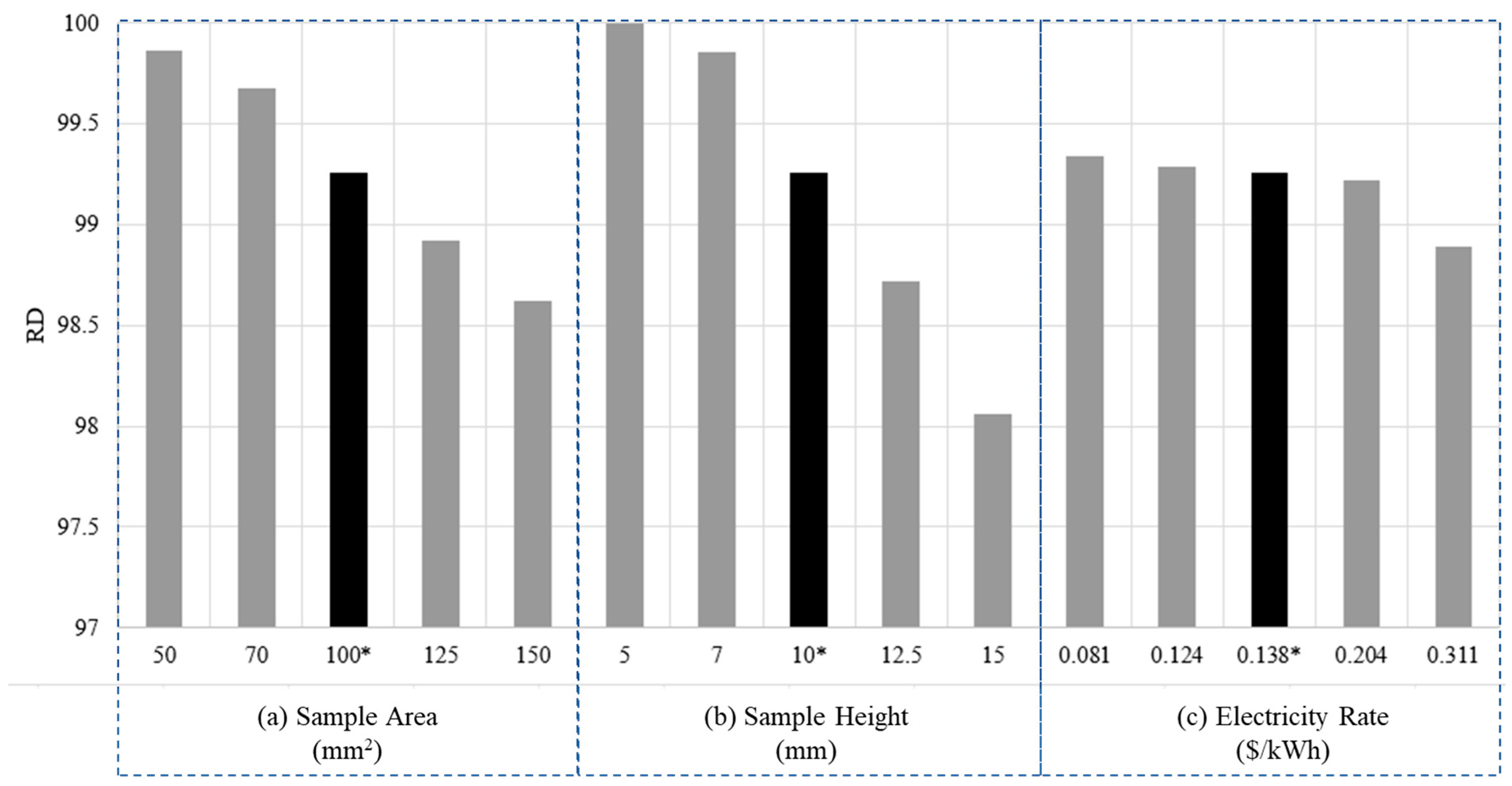
5. Sensitivity Analysis

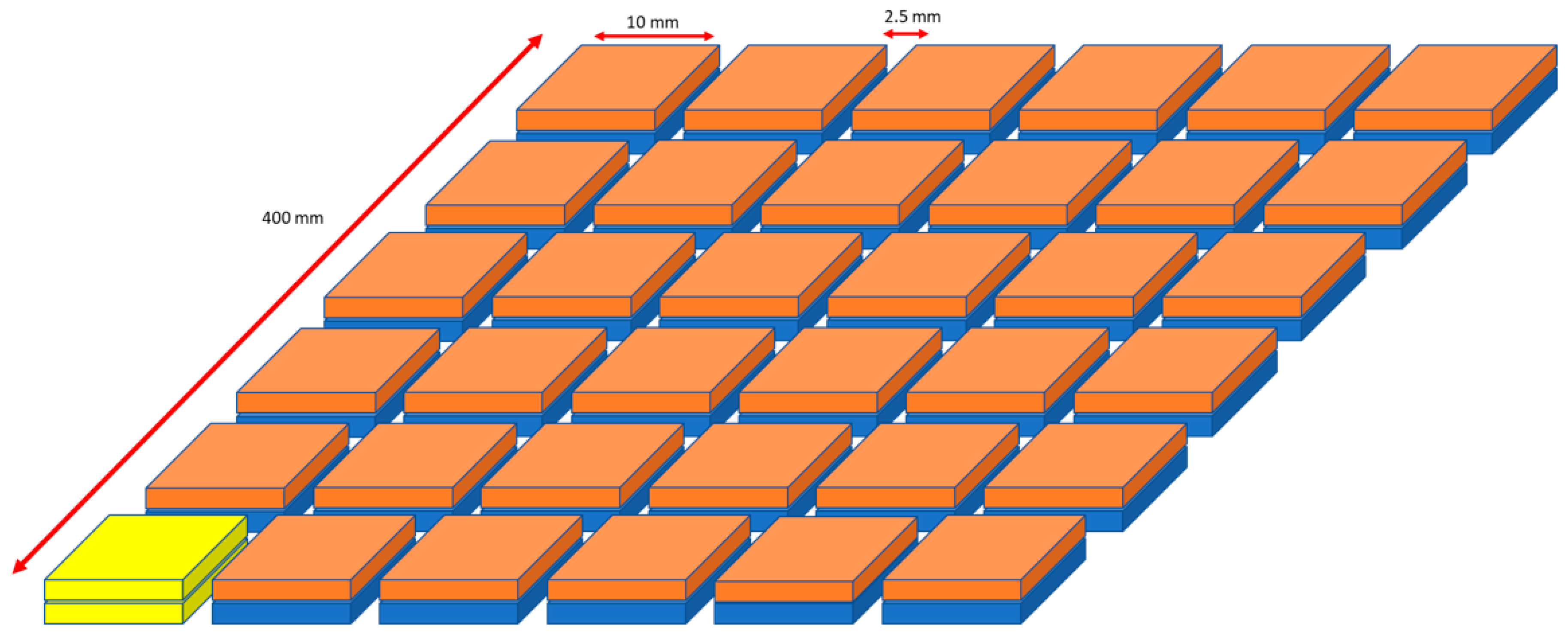
The developed optimization models were built utilizing several assumptions and certain pre-defined model parameters. Thus, it is worth investigating the variation in the quality of the samples through different fabrication scenarios. In particular, the analysis explores the influence of sample area, sample height, and electricity rate on the RD of the built samples, using Model 1. The maximum cost bound remains at USD 1.00 per sample.

Figure 4 demonstrates the overall results of the sensitivity analysis. The centered values marked * in Figure 4 represent the basic cases reported in Section 3. The results indicate that the RD seems to be more sensitive to the sample area and height than the electricity rate. Overall, smaller areas, lower heights, and lower electricity rates generate higher RD. The detailed analyses are presented in the following sub-sections.

5.1. Sample Area

Different areas of the fabricated samples were examined by adjusting only the width of the sample. The length of all specimens remained fixed at 10 mm so that the recoating time per layer ($T_L$) is the same for all cases (i.e., 0.375 s). The solution obtained from Model 1 was based on the assumption that simple cubic samples, each with an area of 100 mm² and a height of 10 mm, were produced. The area of the sample is altered from 100 mm² while other parameters remain the same, resulting in the sample volume change. The results from the variation in the sample area are shown in

Table 7. Results of the variation in the sample area with Model 1.

Sample Area (mm2)	p (W)	v (mm/s)	h (mm)	t (mm)	Layer Thickness (mm)	Fabrication Time (s)			Number of Layers	Machine Operating Cost C0 (USD)	RD (%)
						Scanning	Recoating	Total
50	500	80	420	0.4	0.079	37.721	47.529	85.250	127	1.0000	99.861
70	700	80	420	0.4	0.093	44.899	40.409	85.309	108	1.0007	99.673
100 *	1000	100	444	0.4	0.110	51.140	34.060	85.200	91	0.9994	99.260
125	1250	108	420	0.4	0.131	56.668	28.561	85.228	76	0.9998	98.923
150	1500	120	456	0.4	0.140	58.632	26.709	85.341	71	1.0011	98.621

* The row of sample area 100 m² represents the original optimal solution obtained from Model 1.

.

As the sample area (i.e., width) increases, the optimal solution of Model 1 prescribes higher laser power and a thicker layer. Since the higher layer thickness decreases the required amount of recoating, a reduction in the total recoating time is observed along with the larger sample area (see column Recoating under column Fabrication Time). The total fabrication times are similar, at around 85 s for all sample areas. This may be partly because the machine operating cost per sample is restricted by USD 1.00 for all cases. The RD of the fabricated samples slightly increases as the sample area decreases. It may be related to the USD 1.00 cost limit, which is less tight for smaller samples. Thus, there may be more room in the solution space to increase the RD without exceeding the cost limit for smaller samples.

5.2. Sample Height

The second sensitivity analysis examines the impact of sample height on the optimization solutions. Similar to the variation in the sample area sensitivity analysis, the sample height is altered from the basic case (i.e., 10 mm) while maintaining a fixed area of 100 mm².

Table 8. Results of the variation in sample height with Model 1.

Sample Height (mm)	Sample Volume (mm3)	p (W)	v (mm/s)	h (mm)	t (mm)	Fabrication Time (s)			Number of Layers	Machine Operating Cost C0 (USD)	RD (%)
						Scanning	Recoating	Total
5	500	80	420	0.4	0.0569	52.306	32.9533	85.258	88	1.0325	100.000
7	700	80	420	0.4	0.0796	52.345	32.978	85.322	88	1.0147	99.853
10 *	1000	100	444	0.4	0.1101	51.140	34.060	85.200	91	0.9994	99.260
12.5	1250	112	447	0.4	0.1369	51.087	34.240	85.327	91	0.9946	98.719
15	1500	120	445	0.4	0.1646	51.147	34.174	85.320	91	0.9903	98.059

* The row of sample height 10 mm represents the original optimal solution obtained from Model 1.

presents the results from the variation in the sample height.

Since the sample area is fixed at 100 mm², the scanning time in the XY direction remains very close for all cases, regardless of the sample height change. The recoating time increases with an increase in the sample height because of the increase in the number of layers. Due to the restriction of the cost bound, the total fabrication time is close for all heights to maintain the machine operating cost per sample within USD 1.00. Increasing the sample height results in utilizing a higher laser power, higher scan speed, and larger layer thickness to fabricate bigger samples. As the sample height decreases, the RD increases. Similar to the analysis in the prior section, it may be because, for smaller samples, the USD 1.00 cost limit is less tight, and there may be more room in the solution space to increase the RD without exceeding USD 1.00.

5.3. Electricity Rate

The last part of the sensitivity analysis examines the change in the electricity rate, which is one of the key factors determining the energy consumption cost of an AM machine. Different regions have different electricity rates. Thus, it is essential to understand how the system performs with variations in the rates and the possible effect on the RD of the fabricated samples. As a basic scenario, the commercial electricity rate in the United States, $C_{\mathrm{electricity}}=\mathrm{USD} 0.138$/kWh, was utilized. The rate is then altered to account for different regions using the database in GlobalPetrolPrices.com (accessed on 11 October 2021) [64] and a change in the optimal RD is observed.

Table 9. Results of variation in the electricity rate with Model 1.

Region	Electricity Rate (USD /kWh)	p (W)	v (mm/s)	h (mm)	t (mm)	Fabrication Time (s)			Machine Operating Cost C0 (USD)			RD (%)
						Scanning	Recoating	Total	Fabrication	Energy	Total
UAE	0.081	80	420	0.40	0.111	53.48	33.69	87.17	0.9686	0.0318	1.0004	99.34
Hungary	0.124	80	420	0.40	0.114	52.35	32.98	85.33	0.9481	0.0476	0.9958	99.29
USA *	0.138	100	444	0.40	0.110	51.14	34.06	85.20	0.9467	0.0528	0.9994	99.26
Slovakia	0.204	83	420	0.40	0.117	50.83	32.02	82.86	0.9206	0.0761	0.9967	99.22
Belgium	0.311	94	420	0.39	0.126	48.71	29.88	78.59	0.8732	0.1100	0.9832	98.89

* The row with the USA rate represents the original optimal solution obtained from Model 1.

presents the results.

As the electricity rate increases, the total fabrication time, which is the sum of the scanning and recoating times, decreases to maintain the total cost under the total cost cap at USD 1.00 per sample. Further, a higher electricity rate incurs a higher energy cost, resulting in a lower fabrication cost. However, the energy cost remains a small portion of the total machine operating cost per sample under the considered cost structure. At lower electricity rates, sufficient fabrication time is utilized to scan and recoat the layers properly, achieving high-density samples. In other words, lower electricity rates provide more freedom in utilizing high fabrication time without exceeding the cost limit of USD 1.00 per sample, hence, increasing the RD. As the electricity rate increases, the energy cost increases and a smaller portion of the available cost can be allocated to fabrication. It may be worth noting that the pattern in the prescribed solutions with respect to the electricity rate change is not exactly consistent due to the non-linearity in the system and the random property of the GA used.

5.4. Validation

In order to validate the developed models further, a set of new data from the literature is investigated and used, with process parameter settings outside those used in the development of the model. This ensures that the validation dataset is independent of the datasets used in the training and cross-validation processes. The new experimental data from the literature include the process parameters and the measured RD of SS316L specimens fabricated by different LPBF machines. Using the same process parameters in the literature, the RD is predicted and compared with the experimental data, as presented in

Table 10. Comparison of experimental (literature) and predicted (this work) RD.

Authors	Machine	Laser Power (W)	Scan Speed (mm/s)	Hatch Distance (mm)	Layer Thickness (mm)	Experimental RD from the Literature (%)	Predicted RD by This Work (%)
Ramirez-Cedillo et al. (2020) [65]	Renishaw AM 400	175	300	0.018	0.04	98.93	97.21
		175	188	0.018	0.04	97.80	97.06
		175	300	0.037	0.04	98.85	97.60
		175	188	0.037	0.04	98.02	97.48
		175	300	0.056	0.04	99.27	97.99
		175	188	0.056	0.04	99.54	97.90
Salman et al. (2019) [66]	SLM Solutions 250 H L	175	668	0.12	0.03	99.05	99.08
Huang et al. (2019) [67]	EP-M100T	100	300	0.08	0.02	97.63	96.37
		100	462	0.12	0.02	98.4	98.23
Lin et al. (2019) [68]	Self-developed SLM equipment	150	400	0.08	0.04	99.00	97.35
		150	500	0.08	0.04	99.30	97.05
		150	600	0.08	0.04	98.20	96.67
		150	700	0.08	0.04	95.90	96.22
Röttger et al. (2016) [69]	REALIZER SLM 100	100	400	0.15	0.08	91.20	92.57
Sun et al. (2014) [70]	Renishaw plc	150	125	0.09	0.05	97.00	97.85
		150	150	0.09	0.05	98.30	97.79
		150	175	0.09	0.05	97.00	97.73

.

The results show that there is good agreement between the predicted values and the actual experimental results. Thus, the established model may be reasonably robust and strong enough to be used in future applications.

6. Conclusions

This study presents several multi-performance metric optimization models to efficiently optimize process parameters concerning the RD of 316L stainless-steel specimens fabricated by LPBF. The multivariable regression model with process parameters estimates the RD of the fabricated samples. The machine operating cost is analytically modeled as a function of the process parameters. The study also examines a method to acquire a more stable parameter set and conducts a sensitivity analysis to understand the effect of varying some parameters on the RD of the samples.

The results from 10-fold cross-validation for the developed multivariable regression model demonstrated that the RD could be estimated effectively with an R² of 82.49% and MSE of 4.216. The optimization results showed that samples with RD greater than 99% and a machine operating cost of USD 1.00 per sample can be produced, utilizing a combination of low laser power, high scan speed, moderate layer thickness, and large hatch distance. The addition of penalty terms to the optimization model resulted in more reliable process parameter values. Finally, the sensitivity analysis showed that RD decreases with respect to the increase in sample area, sample height, and electricity rate under the machine operating cost restriction considered.

The approach and methodology followed in this work can be utilized for general purposes and can be extended to other AM materials, and the proposed modeling framework can be applied to other AM techniques. Furthermore, the presented models can be utilized by industrial managers to realize an economically viable AM manufacturing system.

References

1. Shin, D.S.; Lee, C.H.; Kühn, U.; Lee, S.C.; Park, S.J.; Schwab, H.; Scudino, S.; Kosiba, K. Optimizing laser powder bed fusion of Ti-5Al-5V-5Mo-3Cr by artificial intelligence. J. Alloys Compd. 2021, 862, 158018. [Google Scholar] [CrossRef]
2. ISO/ASTM 52900; Additive Manufacturing—General Principles and Terminology. ISO/ASTM International: West Conshohocken, PA, USA, 2015; Volume 5, pp. 1–26.
3. Shi, X.; Ma, S.; Liu, C.; Chen, C.; Wu, Q.; Chen, X.; Lu, J. Performance of high layer thickness in selective laser melting of Ti6Al4V. Materials 2016, 9, 975. [Google Scholar] [PubMed] [Green Version]
4. Ahmed, N.; Barsoum, I.; Haidemenopoulos, G.; Al-Rub, R.K.A. Process parameter selection and optimization of laser powder bed fusion for 316L stainless steel: A review. J. Manuf. Process. 2022, 75, 415–434. [Google Scholar] [CrossRef]
5. Ahmed, N.; Barsoum, I.; Abu Al-Rub, R.K. Numerical Investigation on the Effect of Residual Stresses on the Effective Mechanical Properties of 3D-Printed TPMS Lattices. Metals 2022, 12, 1344. [Google Scholar]
6. Murr, L.E.; Gaytan, S.M.; Ramirez, D.A.; Martinez, E.; Hernandez, J.; Amato, K.N.; Shindo, P.W.; Medina, F.R.; Wicker, R.B. Metal Fabrication by Additive Manufacturing Using Laser and Electron Beam Melting Technologies. J. Mater. Sci. Technol. 2012, 28, 1–14. [Google Scholar] [CrossRef]
7. Garg, A.; Tai, K.; Savalani, M.M. State-of-the-art in empirical modelling of rapid prototyping processes. Rapid Prototyp. J. 2014, 20, 164–178. [Google Scholar] [CrossRef]
8. Srivastava, M.; Maheshwari, S.; Kundra, T.; Rathee, S. Multi-Response Optimization of Fused Deposition Modelling Process Parameters of ABS Using Response Surface Methodology (RSM)-Based Desirability Analysis. Mater. Today Proc. 2017, 4, 1972–1977. [Google Scholar]
9. AlFaify, A.; Hughes, J.; Ridgway, K. Controlling the porosity of 316L stainless steel parts manufactured via the powder bed fusion process. Rapid Prototyp. J. 2019, 25, 162–175. [Google Scholar] [CrossRef]
10. Marrey, M.; Malekipour, E.; El-Mounayri, H.; Faierson, E.J. A framework for optimizing process parameters in powder bed fusion (PBF) process using artificial neural network (ANN). Procedia Manuf. 2019, 34, 505–515. [Google Scholar] [CrossRef]
11. Rong-Ji, W.; Xin-Hua, L.; Qing-Ding, W.; Lingling, W. Optimizing process parameters for selective laser sintering based on neural network and genetic algorithm. Int. J. Adv. Manuf. Technol. 2009, 42, 1035–1042. [Google Scholar] [CrossRef]
12. Saad, M.S.; Nor, A.M.; Baharudin, M.E.; Zakaria, M.Z.; Aiman, A.F. Optimization of surface roughness in FDM 3D printer using response surface methodology, particle swarm optimization, and symbiotic organism search algorithms. Int. J. Adv. Manuf. Technol. 2019, 105, 5121–5137. [Google Scholar] [CrossRef]
13. Read, N.; Wang, W.; Essa, K.; Attallah, M.M. Selective laser melting of AlSi10Mg alloy: Process optimisation and mechanical properties development. Mater. Des. 2015, 65, 417–424. [Google Scholar] [CrossRef]
14. Laakso, P.; Riipinen, T.; Laukkanen, A.; Andersson, T.; Jokinen, A.; Revuelta, A.; Ruusuvuori, K. Optimization and simulation of SLM process for high density H13 tool steel parts. Phys. Procedia 2016, 83, 26–35. [Google Scholar]
15. Aboutaleb, A.M.; Bian, L.; Elwany, A.; Shamsaei, N.; Thompson, S.M.; Tapia, G. Accelerated process optimization for laser-based additive manufacturing by leveraging similar prior studies. IISE Trans. 2017, 49, 31–44. [Google Scholar] [CrossRef]
16. Bai, Y.; Yang, Y.; Xiao, Z.; Zhang, M.; Wang, D. Process optimization and mechanical property evolution of AlSiMg0.75 by selective laser melting. Mater. Des. 2018, 140, 257–266. [Google Scholar] [CrossRef]
17. Mao, Z.; Zhang, D.Z.; Jiang, J.; Fu, G.; Zhang, P. Processing optimisation, mechanical properties and microstructural evolution during selective laser melting of Cu-15Sn high-tin bronze. Mater. Sci. Eng. A 2018, 721, 125–134. [Google Scholar] [CrossRef] [Green Version]
18. Yakout, M.; Elbestawi, M.A.; Veldhuis, S.C. Density and mechanical properties in selective laser melting of Invar 36 and stainless steel 316L. J. Mater. Process. Technol. 2019, 266, 397–420. [Google Scholar] [CrossRef]
19. Vallejo, N.D.; Lucas, C.; Ayers, N.; Graydon, K.; Hyer, H.; Sohn, Y. Process optimization and microstructure analysis to understand laser powder bed fusion of 316l stainless steel. Metals 2021, 11, 832. [Google Scholar] [CrossRef]
20. Majeed, A.; Lv, J.; Zhang, Y.; Muzamil, M.; Waqas, A.; Shamim, K.; Qureshi, M.E.; Zafar, F. An investigation into the influence of processing parameters on the surface quality of AlSi10Mg parts by SLM process. In Proceedings of the 2019 16th International Bhurban Conference on Applied Sciences and Technology (IBCAST), Islamabad, Pakistan, 8–12 January 2019; pp. 143–147. [Google Scholar]
21. Samantaray, M.; Thatoi, D.N.; Sahoo, S. Modeling and Optimization of Process Parameters for Laser Powder Bed Fusion of AlSi10Mg Alloy. Lasers Manuf. Mater. Process. 2019, 6, 356–373. [Google Scholar] [CrossRef]
22. Arısoy, Y.M.; Criales, L.E.; Özel, T.; Lane, B.; Moylan, S.; Donmez, A. Influence of scan strategy and process parameters on microstructure and its optimization in additively manufactured nickel alloy 625 via laser powder bed fusion. Int. J. Adv. Manuf. Technol. 2017, 90, 1393–1417. [Google Scholar] [CrossRef]
23. Shi, W.; Wang, P.; Liu, Y.; Hou, Y.; Han, G. Properties of 316L formed by a 400 W power laser Selective Laser Melting with 250 μm layer thickness. Powder Technol. 2020, 360, 151–164. [Google Scholar] [CrossRef]
24. Maamoun, A.H.; Xue, Y.F.; Elbestawi, M.A.; Veldhuis, S.C. Effect of selective laser melting process parameters on the quality of al alloy parts: Powder characterization, density, surface roughness, and dimensional accuracy. Materials 2018, 11, 2343. [Google Scholar] [CrossRef] [PubMed] [Green Version]
25. Mutua, J.; Nakata, S.; Onda, T.; Chen, Z.C. Optimization of selective laser melting parameters and influence of post heat treatment on microstructure and mechanical properties of maraging steel. Mater. Des. 2018, 139, 486–497. [Google Scholar] [CrossRef]
26. Aboutaleb, A.M.; Mahtabi, M.; Tschopp, M.A.; Bian, L. Multi-objective accelerated process optimization of mechanical properties in laser-based additive manufacturing: Case study on Selective Laser Melting (SLM) Ti-6Al-4V. J. Manuf. Process. 2019, 38, 432–444. [Google Scholar] [CrossRef]
27. Wang, C.; Tan, X.; Liu, E.; Tor, S.B. Process parameter optimization and mechanical properties for additively manufactured stainless steel 316L parts by selective electron beam melting. Mater. Des. 2018, 147, 157–166. [Google Scholar] [CrossRef]
28. Deng, Y.; Mao, Z.; Yang, N.; Niu, X.; Lu, X. Collaborative optimization of density and surface roughness of 316L stainless steel in selective laser melting. Materials 2020, 13, 1601. [Google Scholar] [CrossRef] [PubMed] [Green Version]
29. Sun, J.; Shen, L.; Wang, W.; Liu, Z.; Chen, H.; Duan, J. Study of Microstructure and Properties of 316L with Selective Laser Melting Based on Multivariate Interaction Influence. Adv. Mater. Sci. Eng. 2020, 2020, 8404052. [Google Scholar] [CrossRef] [Green Version]
30. Pant, P.; Chatterjee, D.; Nandi, T.; Samanta, S.K.; Lohar, A.K.; Changdar, A. Statistical modelling and optimization of clad characteristics in laser metal deposition of austenitic stainless steel. J. Brazilian Soc. Mech. Sci. Eng. 2019, 41, 1–10. [Google Scholar] [CrossRef]
31. Bonakdar, A.; Liravi, F.; Toyserkani, E.; Ali, U.; Mahmoodkhani, Y. Method and System for Optimzing Process Parameters in an Additive Manufacturing Process. U.S. Patent Application No 17/599,392, 9 June 2022. [Google Scholar]
32. Vyavahare, S.; Teraiya, S.; Panghal, D.; Kumar, S. Fused deposition modelling: A review. Rapid Prototyp. J. 2020, 26, 176–201. [Google Scholar]
33. Abdulla, H.; Maalouf, M.; Barsoum, I.; An, H. Truncated Newton Kernel Ridge Regression for Prediction of Porosity in Additive Manufactured SS316L. Appl. Sci. 2022, 12, 4252. [Google Scholar] [CrossRef]
34. Kamath, C.; El-Dasher, B.; Gallegos, G.F.; King, W.E.; Sisto, A. Density of additively-manufactured, 316L SS parts using laser powder-bed fusion at powers up to 400 W. Int. J. Adv. Manuf. Technol. 2014, 74, 65–78. [Google Scholar] [CrossRef] [Green Version]
35. Spierings, A.B.; Herres, N.; Levy, G. Influence of the particle size distribution on surface quality and mechanical properties in AM steel parts. Rapid Prototyp. J. 2020, 17, 195–202. [Google Scholar] [CrossRef] [Green Version]
36. Choi, J.P.; Shin, G.H.; Brochu, M.; Kim, Y.J.; Yang, S.S.; Kim, K.T.; Yang, D.Y.; Lee, C.W.; Yu, J.H. Densification behavior of 316L stainless steel parts fabricated by selective laser melting by variation in laser energy density. Mater. Trans. 2016, 57, 1952–1959. [Google Scholar] [CrossRef] [Green Version]
37. Greco, S.; Gutzeit, K.; Hotz, H.; Kirsch, B.; Aurich, J.C. Selective laser melting (SLM) of AISI 316L—Impact of laser power, layer thickness, and hatch spacing on roughness, density, and microhardness at constant input energy density. Int. J. Adv. Manuf. Technol. 2020, 108, 1551–1562. [Google Scholar] [CrossRef]
38. Leicht, A.; Rashidi, M.; Klement, U.; Hryha, E. Effect of process parameters on the microstructure, tensile strength and productivity of 316L parts produced by laser powder bed fusion. Mater. Charact. 2020, 159, 110016. [Google Scholar] [CrossRef]
39. Larimian, T.; Kannan, M.; Grzesiak, D.; AlMangour, B.; Borkar, T. Effect of energy density and scanning strategy on densification, microstructure and mechanical properties of 316L stainless steel processed via selective laser melting. Mater. Sci. Eng. A 2020, 770, 138455. [Google Scholar] [CrossRef]
40. Tucho, W.M.; Lysne, V.H.; Austbø, H.; Sjolyst-Kverneland, A.; Hansen, V. Investigation of effects of process parameters on microstructure and hardness of SLM manufactured SS316L. J. Alloys Compd. 2018, 740, 910–925. [Google Scholar] [CrossRef]
41. Peng, T.; Chen, C. Influence of energy density on energy demand and porosity of 316L stainless steel fabricated by selective laser melting. Int. J. Precis. Eng. Manuf.-Green Technol. 2018, 5, 55–62. [Google Scholar] [CrossRef]
42. Cherry, J.A.; Davies, H.M.; Mehmood, S.; Lavery, N.P.; Brown, S.G.R.; Sienz, J. Investigation into the effect of process parameters on microstructural and physical properties of 316L stainless steel parts by selective laser melting. Int. J. Adv. Manuf. Technol. 2014, 76, 869–879. [Google Scholar] [CrossRef] [Green Version]
43. Wang, D.; Liu, Y.; Yang, Y.; Xiao, D. Theoretical and experimental study on surface roughness of 316L stainless steel metal parts obtained through selective laser melting. Rapid Prototyp. J. 2016, 22, 706–716. [Google Scholar] [CrossRef]
44. Raj, S.; Kannan, S. Detection of Outliers in Regression Model for Medical Data. Int. J. Med. Res. Health Sci. 2017, 6, 50–56. [Google Scholar]
45. Miranda, G.; Faria, S.; Bartolomeu, F.; Pinto, E.; Madeira, S.; Mateus, A.; Carreira, P.; Alves, N.; Silva, F.S.; Carvalho, O. Predictive models for physical and mechanical properties of 316L stainless steel produced by selective laser melting. Mater. Sci. Eng. A 2016, 657, 43–56. [Google Scholar] [CrossRef]
46. Barrionuevo, G.O.; Ramos-Grez, J.A.; Walczak, M.; Betancourt, C.A. Comparative evaluation of supervised machine learning algorithms in the prediction of the relative density of 316L stainless steel fabricated by selective laser melting. Int. J. Adv. Manuf. Technol. 2021, 113, 419–433. [Google Scholar] [CrossRef]
47. de Rooij, M.; Weeda, W. Cross-Validation: A Method Every Psychologist Should Know. Adv. Methods Pract. Psychol. Sci. 2020, 3, 248–263. [Google Scholar] [CrossRef]
48. Fauth, J.; Elkaseer, A.; Scholz, S.G. Total Cost of Ownership for Different State of the Art FDM Machines (3D Printers); Springer: Singapore, 2019; Volume 155, ISBN 9789811392702. [Google Scholar]
49. Jumani, M.S.; Shaikh, S.; Shah, S.A. Fused deposition modelling technique (FDM) for fabrication of custom-made foot orthoses: A cost and benefit analysis. Sci.Int. 2014, 26, 2571–2576. [Google Scholar]
50. Hopkinson, N.; Dickens, P. Analysis of rapid manufacturing—Using layer manufacturing processes for production. Proc. Inst. Mech. Eng. Part C J. Mech. Eng. Sci. 2015, 217, 31–39. [Google Scholar] [CrossRef]
51. Mahadik, A.; Masel, D. Implementation of Additive Manufacturing Cost Estimation Tool (AMCET) Using Break-down Approach. Procedia Manuf. 2018, 17, 70–77. [Google Scholar] [CrossRef]
52. Di, L.; Yang, Y. Cost modeling and evaluation of direct metal laser sintering with integrated dynamic process planning. Sustainability 2021, 13, 319. [Google Scholar] [CrossRef]
53. Zhang, L.C.; Wang, J.; Liu, Y.; Jia, Z.; Liang, S.X. Additive Manufacturing of Titanium Alloys; Elsevier: Amsterdam, The Netherlands, 2022; Volume 1, ISBN 9780128197264. [Google Scholar]
54. Song, X.; Zhai, W.; Huang, R.; Fu, J.; Fu, M.W.; Li, F. Metal-Based 3D-Printed Micro Parts & Structures; Elsevier: Amsterdam, The Netherlands, 2022; Volume 4, ISBN 9780128197264. [Google Scholar]
55. EOS GmbH. Large and Ultra-Fast 3D Printer with 4 Laser. 2019. Available online: https://www.eos.info/en/additive-manufacturing/3d-printing-metal/eos-metal-systems/eos-m-400-4 (accessed on 15 September 2021).
56. Liu, Z.Y.; Li, C.; Fang, X.Y.; Guo, Y.B. Energy Consumption in Additive Manufacturing of Metal Parts. Procedia Manuf. 2018, 26, 834–845. [Google Scholar] [CrossRef]
57. An, H.; Byon, Y.J.; Cho, C.S. Economic and Environmental Evaluation of a Brick Delivery System Based on Multi-Trip Vehicle Loader Routing Problem for Small Construction Sites. Sustainability 2018, 10, 1427. [Google Scholar] [CrossRef] [Green Version]
58. Piili, H.; Happonen, A.; Väistö, T.; Venkataramanan, V.; Partanen, J.; Salminen, A. Cost Estimation of Laser Additive Manufacturing of Stainless Steel. Phys. Procedia 2015, 78, 388–396. [Google Scholar] [CrossRef]
59. Diegel, O.; Wohlers, T.; Collins, F. Component Design for Cost-Efficient Metal Additive Manufacturing. 2018. Available online: https://www.metal-am.com/articles/component-design-for-cost-efficient-metal-3d-printing/ (accessed on 13 September 2021).
60. ChooseEnergy. Electricity Rates by State (July 2021)|ChooseEnergy.com®. 2021. Available online: https://www.chooseenergy.com/electricity-rates-by-state/ (accessed on 13 September 2021).
61. Onler, R.; Koca, A.S.; Kirim, B.; Soylemez, E. Multi-objective optimization of binder jet additive manufacturing of Co-Cr-Mo using machine learning. Int. J. Adv. Manuf. Technol. 2021, 119, 1091–1108. [Google Scholar] [CrossRef]
62. Vosniakos, G.C.; Maroulis, T.; Pantelis, D. A method for optimizing process parameters in layer-based rapid prototyping. Proc. Inst. Mech. Eng. Part B J. Eng. Manuf. 2007, 221, 1329–1340. [Google Scholar] [CrossRef]
63. An, H.; Choi, S.; Lee, J.H. Integrated scheduling of vessel dispatching and port operations in the closed-loop shipping system for transporting petrochemicals. Comput. Chem. Eng. 2019, 126, 485–498. [Google Scholar] [CrossRef]
64. Electricity Prices around the World | GlobalPetrolPrices.com. 2021. Available online: http://GlobalPetrolPrices.com (accessed on 11 October 2021).
65. Ramirez-Cedillo, E.; Uddin, M.J.; Sandoval-Robles, J.A.; Mirshams, R.A.; Ruiz-Huerta, L.; Rodriguez, C.A.; Siller, H.R. Process planning of L-PBF of AISI 316L for improving surface quality and relating part integrity with microstructural characteristics. Surf. Coatings Technol. 2020, 396, 125956. [Google Scholar] [CrossRef]
66. Salman, O.O.; Brenne, F.; Niendorf, T.; Eckert, J.; Prashanth, K.G.; He, T.; Scudino, S. Impact of the scanning strategy on the mechanical behavior of 316L steel synthesized by selective laser melting. J. Manuf. Process. 2019, 45, 255–261. [Google Scholar] [CrossRef]
67. Qi, X.; Feng, H.; Liu, L. Effect of selective laser melting process parameters on microstructure and mechanical properties of 316L stainless steel helical micro-diameter spring. AIP Conf. Proc. 2019, 2154, 2117–2131. [Google Scholar] [CrossRef]
68. Lin, K.; Gu, D.; Xi, L.; Yuan, L.; Niu, S.; Lv, P.; Ge, Q. Selective laser melting processing of 316L stainless steel: Effect of microstructural differences along building direction on corrosion behavior. Int. J. Adv. Manuf. Technol. 2019, 104, 2669–2679. [Google Scholar] [CrossRef]
69. Röttger, A.; Geenen, K.; Windmann, M.; Binner, F.; Theisen, W. Comparison of microstructure and mechanical properties of 316 L austenitic steel processed by selective laser melting with hot-isostatic pressed and cast material. Mater. Sci. Eng. A 2016, 678, 365–376. [Google Scholar] [CrossRef]
70. Sun, Y.; Moroz, A.; Alrbaey, K. Sliding wear characteristics and corrosion behaviour of selective laser melted 316L stainless steel. J. Mater. Eng. Perform. 2014, 23, 518–526. [Google Scholar] [CrossRef]
Figure 1. Schematic diagram of the process of the methods used in this study.
Metals 12 02098 g001
Figure 2. Sample layout in the chamber of EOS M 400 system.
Metals 12 02098 g002
Figure 3. Comparison of variation in relative density with change in cost bound for Model 1 and Model 1′.
Metals 12 02098 g003
Figure 4. Sensitivity analysis of relative density with change in (a) sample area, (b) sample height, and (c) electricity rate, using Model 1.
Metals 12 02098 g004