Review

Plastic Deformation Behavior of Metal Materials: A Review of Constitutive Models

College of Mechanical and Electrical Engineering, Nanjing Forestry University, Nanjing 210037, China
*
Author to whom correspondence should be addressed.
Metals 2022, 12(12), 2077; https://doi.org/10.3390/met12122077
Submission received: 22 October 2022 / Revised: 25 November 2022 / Accepted: 30 November 2022 / Published: 3 December 2022

Abstract

:
The deformation behavior of metal materials in plastic forming is intimately related to deformation conditions, which are greatly affected by deformation rate, forming temperature, and plastic variables. Macroscopic mechanical properties research is an important basis and technical means to analyze the process parameters and deformation process of metal plastic forming. Therefore, to reveal the influence mechanism of macroscopic mechanical properties of metal materials, and establish material constitutive models under different deformation conditions, it is of great significance to choose reasonable forming parameters and prevent forming defects. There are substantial variances in the macroscopic mechanical characteristics of different materials in the deformation process. In order to accurately predict its deformation behavior, the phenomenological constitutive model, the microscopic constitutive model reflecting the microscopic deformation mechanism, and the artificial neural network constitutive model based on the neural network were constructed respectively on the basis of macroscopic mechanical tests and microscopic microstructure tests. On the basis of the existing research results, the advantages and disadvantages of phenomenological constitutive model, microscopic constitutive model, and neural network constitutive model are compared and analyzed, respectively. The research results of this paper will provide support for the selection of constitutive models for reasonably predicting the deformation behavior of metal materials.

1. Introduction

In recent years, with the rapid development of aviation, space flight, automobile and other fields, higher requirements have been put forward for the forming quality and service life of metal parts. The metal plastic forming process is the main forming technology for thin-walled and key stressed parts. Therefore, the formulation of suitable process parameters based on the plastic deformation behavior of materials is the key to the quality control of metal plastic forming [1,2].
In the process of metal plastic forming, the flow behavior of material is highly affected by deformation temperature, deformation velocity, and deformation amount. Especially in the thermoplastic forming process, the plastic deformation behavior of the material is the result of the combined action of work hardening and temperature softening, and is greatly affected by strain, strain rate, and forming temperature. On the one hand, under the conditions of given thermodynamic parameters, the deformation of materials is accompanied by microstructure evolution; on the other hand, the change of microstructure during plastic deformation also causes the change of flow stress of materials. Therefore, revealing the plastic deformation mechanism of metal materials under complicated deformation conditions is of great significance for the formulation and optimization of reasonable plastic forming process parameters [3,4,5,6,7].
In order to accurately predict the flow behavior of metal materials under deformation, a large number of studies have been carried out in recent years, and constitutive models have been established on this basis; the constitutive models can describe the effects of strain rate, forming temperature, strain and strain rate on the deformation behavior of materials during deformation. However, due to the obvious nonlinear characteristics of the plastic deformation behavior of the material during the plastic deformation process, it is difficult for a single constitutive model to fully describe the influence of all deformation parameters [8].
Therefore, it is the focus of research on material deformation behavior to create new constitutive models or alter existing constitutive models with the use of macroscopic and microscopic test data. Nonlinear flow behavior of different metals or alloys under many impact factors consider the particular influence of deformation process parameters.
In the plastic deformation process, the change of microstructure is the main reason for the change of macroscopic mechanical properties under different deformation conditions. When the deformation reaches a certain degree, with the increase of deformation, the microscopic damage of the material continues to accumulate and expand [8], which makes the macroscopic mechanical properties of the material change significantly.
The accumulation of damage during plastic deformation is the main cause of forming failure, which will also lead to premature fatigue failure of parts. Therefore, the prediction of plastic deformation damage accumulation is also an important factor to be considered in the design of forming process parameters. The damage evolution of metal materials during plastic deformation can be separated into two components: one is the growth of the original hole of the material, and the other is the nucleation and growth of new holes during deformation. Based on continuum damage theory, the accumulation of stress–strain is the main factor of plastic deformation damage. With the development of the research on the plastic deformation damage theory, the research on the deformation behavior of materials gradually changes from macro to micro. In the establishment of the constitutive model, in addition to considering the macroscopic deformation characteristics, the microscopic parameters are gradually introduced to characterize the microscopic deformation mechanism of materials.
The most commonly used constitutive models can be divided into three categories: phenomenological model, microscopic model, and artificial neural network model [9,10]. Because of few parameters and it being easy to be established, the phenomenological model is the most important model in the engineering application, such as the Arrhenius constitutive equation, the Johnson–Cook (J–C) model, Fields–Backofen (FB) Model, Hansel–Spittel Model, and Molinari–Ravichandran Model. However, the phenomenological model cannot directly reflect the influence of material microscopic parameters on macroscopic mechanical properties. The microscopic model is based on the microscopic deformation mechanism of materials, such as the Zerilli–Armstrong Model (ZA Model), Preston–Tonks–Wallace (PTW) Model, Rusinek–Klepaczko (RK) Model, and the Cellular Automaton (CA) Model. Although the microscopic model directly reflects the influence of the microscopic parameters on the macroscopic performance, the microscopic model has more parameters compared with the phenomenological model, and it is more difficult to determine the model parameters. The artificial neural network model can be used to predict the flow stress of materials under complex deformation conditions, which avoids the difficult problem of material parameter determination of the traditional constitutive model, and is suitable for finite element simulation of the material deformation process.

2. Phenomenological Model

Based on the experimental data, the phenomenological model can determine the influence of stress, strain, temperature, and strain rate on the material deformation behavior through data fitting and other technical means, so as to construct a constitutive relationship model that can reflect the macroscopic deformation behavior of materials. Although the parameters of the phenomenological model are relatively few, it is easy to obtain by experimental means, and the phenomenological model does not consider the influence of material composition, grain size, dislocation density, and other factors on material properties. Therefore, it cannot reveal the micro-deformation mechanism of materials, which limits the application of the model. Usually, the prediction accuracy of the phenomenological model is high in the limited strain rate and temperature range, and the model cannot accurately reflect the deformation behavior of the material after exceeding the range.

2.1. Johnson–Cook (J–C) Model

The Johnson–Cook model (J–C) is a typical representative of the phenomenological model, which is widely used in industrial production and material property prediction research [11]. As shown in Equation (1), the J–C model assumes that the material is isotropic and decouples the work hardening effect, strain rate effect, and temperature effect to simplify the constitutive equation, and the parameters of J–C model can be calibrated by uniaxial tensile or compressive tests of materials:
σ e = ( A + B ε p n ) ( 1 + C ln ε ˙ ε ˙ 0 ) [ 1 ( T T 0 T m T 0 ) m ]
where σe is the Von-Mises equivalent stress, A is the yield stress (MPa) under the reference strain rate, B is the hardening coefficient (MPa), C is the strain rate sensitivity coefficient, n is the hardening exponent, m is the temperature sensitivity coefficient, εp is the equivalent plastic strain, ε ˙ is the strain rate (s−1), ε p is the reference strain rate (s−1), T is the actual temperature, T0 is the ambient temperature, and Tm is the melting point temperature of the material.
When the deformation temperature T of the material is basically the same as the ambient temperature T0, and the material is loaded under quasi-static conditions, the flow stress of the material only needs to consider the effect of strain hardening on the stress. Thus, the J–C model can be simplified as
σ e = ( A + B ε p n )
The relationship between the equivalent stress σe and the equivalent plastic strain εp in Equation (2) can be adapted to all stress states, and the three parameters A, B, and n are coupled with each other.
The material parameters in the J–C model can be determined by fitting with less experimental data; however, this will not take into account the influence of complex stress states on material properties. When the traditional model parameter calibration method is used to determine the model parameters, there will be a large error between the numerical simulation results and the actual deformation of the material under complex stress conditions. In order to reduce this difference, Ru [12] took 6005A-T6 aluminum alloy as the research object and obtained the optimal solution of J–C model parameters based on the test data under different stress states with the help of the inversion calibration method based on a genetic algorithm.
The J–C model assumes that thermal softening, strain rate hardening, and strain hardening are three independent phenomena, which can be isolated from each other without considering the effect of the interaction among the three. That is to say, the original J–C model does not include any historical effect of thermal or strain rate. Although the J–C model can easily realize the calibration of parameters, it can only describe the relationship at the macro level such as strain rate, temperature, flow stress, and strain. It lacks the essence of material deformation and cannot describe the flow stress of material from the micro deformation mechanism of material. It can only describe the relationship of strain rate, temperature, flow stress, and strain at the macroscopic level, but cannot represent the microscopic deformation mechanism of the material.
Zhang [13] modified the original J–C model by considering the effect of forming temperature on strain hardening behavior of IC10 alloy. The modified J–C model can be expressed as
σ e = [ A ( 1 T T 0 T m T 0 ) + B ( T ) ε p n ] ( 1 + C ln ε ˙ ε ˙ 0 )
where
T * = T T 0 T m T 0
B ( T * ) is a temperature effect function, which can be defined as
B ( T ) = σ b r ( 1 T m 1 ) σ 0.2 r ( 1 T m ) ( ε b r ( 1 + P 1 × T P 2 × T P 3 ) ) n
where m1, P1, P2, and P3 are material constants. σbr is the fracture stress at room temperature. εbr is the fracture strain at room temperature.
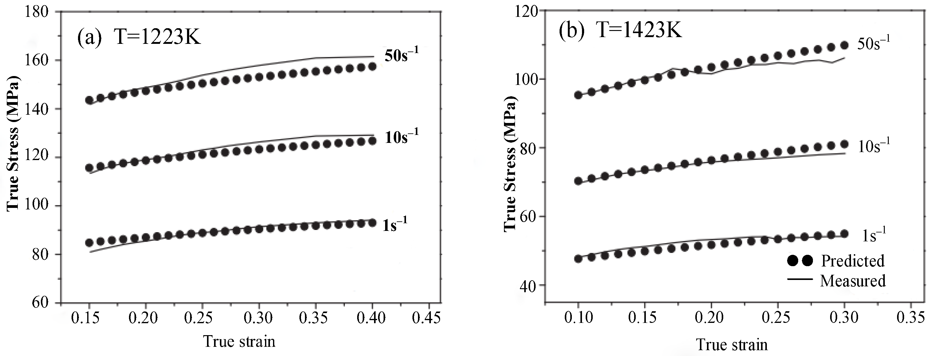
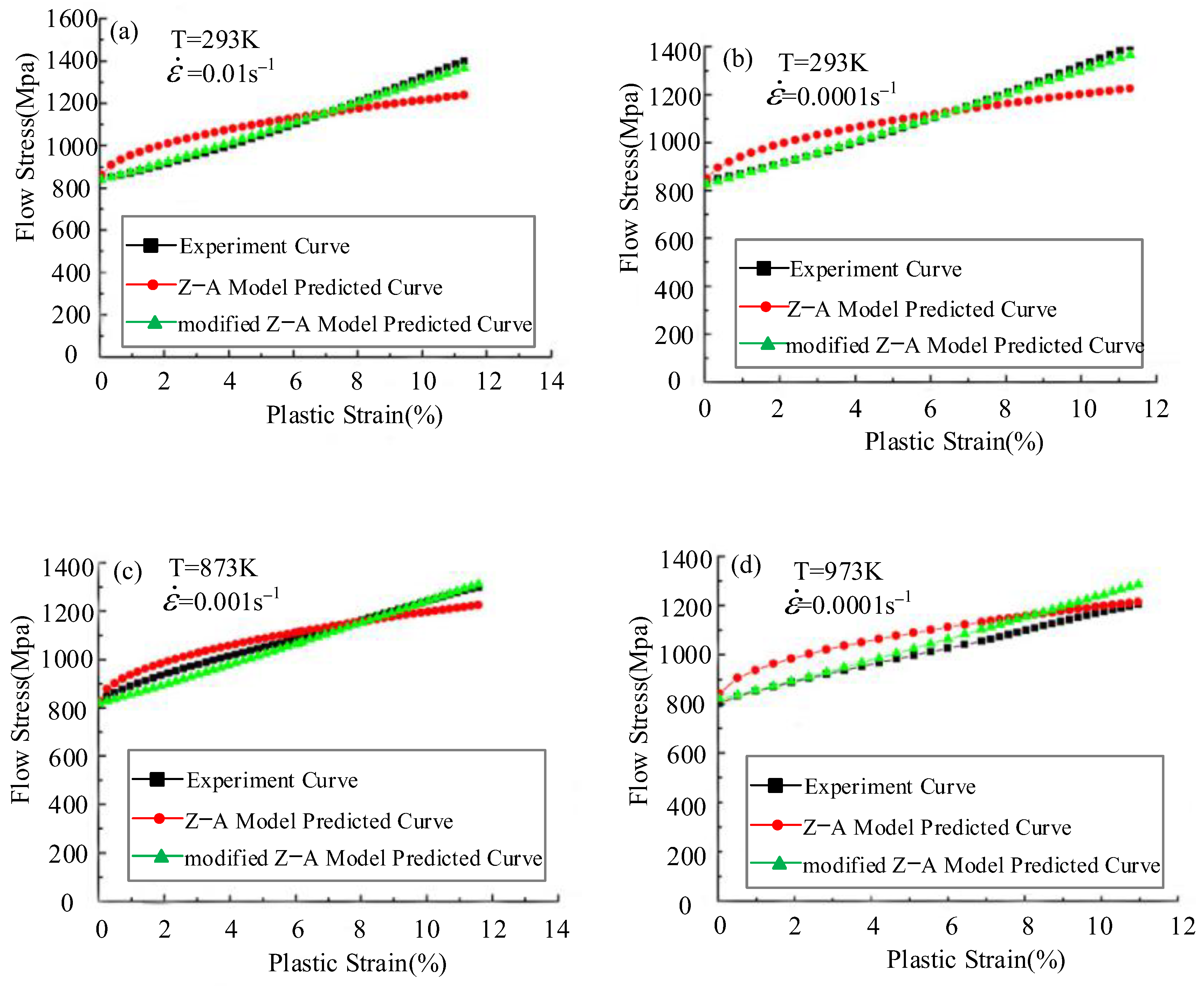
The flow stress of IC10 alloy was fitted by the modified J–C model, and the fitting results are shown in Figure 1. The results show that the flow stress predicted by the modified J–C model is in good agreement with the experimental results, but the prediction accuracy is poor when the temperature is 800 °C, and the strain rate is 0.0001 s−1.
Lin and Chen [14] studied the deformation behavior of 42CrMo alloy steel under hot compression based on Johnson–Cook and Zerili–Armstrong (JC–ZA) coupled model, and established the relationship between flow stress, strain rate, and forming temperature:
σ = ( A + B ε n ) exp ( C 3 T + C 4 T ε ˙ )  
where A, B, n, C3, and C4 are material parameters. σ is equivalent stress. ε is equivalent strain. T is the absolute temperature. ε ˙ * = ε ˙ / ε ˙ 0 is dimensionless strain rate.
Since about 3–5% plastic deformation energy is retained in the material as storage energy, this will increase the temperature of the sample; thus, Equation (6) can be modified to
σ = ( A 1 + B 1 ε n ) exp [ C 3 ( T + Δ T ) + C 4 ( T + Δ T ) ln ε ˙ ]
The flow stress of 42CrMo steel obtained by JC-ZA is shown in Figure 2. Since the JC-ZA model not only considers the strain hardening phenomena, but also considers the coupling effect of temperature and strain rate on the flow behavior, the accuracy of the prediction results of the model is improved.
Under the condition of high strain rate, since the thermal effect of plastic deformation is significantly correlated with the strain rate, the original J–C model cannot reflect the strain rate effect under the high strain rate. Therefore, the prediction accuracy of J–C model will be reduced. To solve this problem, Vural and Caro [15] modified the strain rate sensitivity parameter C in J–C model to improve the prediction accuracy of the model. The modified J–C model of Vural and Caro makes temperature directly couple with strain hardening.
C = C 1 ( T r ) p + C 2 H ( ε ˙ , ε ˙ t , k )
H ( ε ˙ , ε ˙ t , k ) = 1 2 + 1 2 tanh ( k ln ε ˙ ε ˙ t ) = 1 1 + e 2 k ln ( ε ˙ / ε ˙ t )
T * = T T r T r T r
where T is room temperature. Tr is the reference temperature. C1 represents the rate sensitivity parameter ( ε ˙ < ε ˙ t ) under quasi-static strain rate at room temperature. C2 represents the increase of rate sensitivity parameter under dynamic strain rate, which is the transition strain rate ( ε ˙ > ε ˙ t ) between quasi-static deformation zone and dynamic deformation zone, usually 102–103 s−1. H ( ε ˙ , ε ˙ t , k ) is the smooth approximation of the Heaviside step function and changes continuously near the transition strain rate. k is the proportional factor.
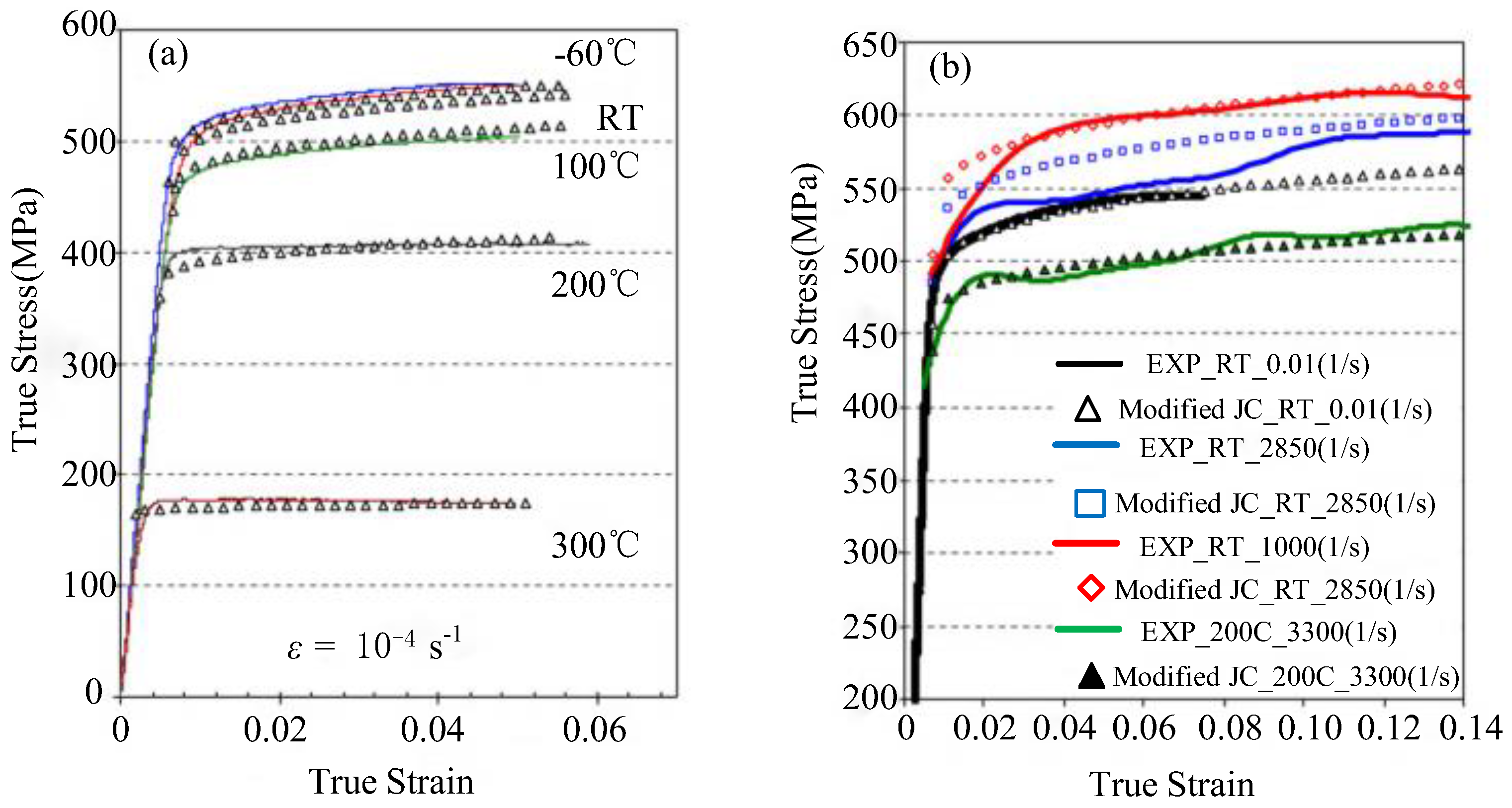
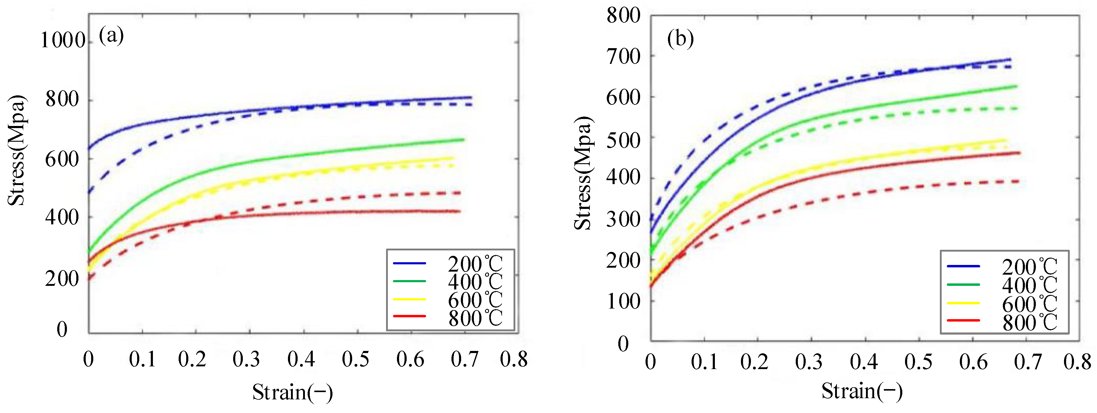
Based on the tensile tests and compressive tests, Vural and Caro [15] determined the parameters of the modified J–C model of 2139 Aluminum Alloys. By enhancing the coupling effect between temperature and strain hardening, the flow stress changes related to rate and temperature were better captured, as shown in Figure 3. Comparing the tensile test results with the compression test results, the strain rate sensitivity under dynamic state is enhanced through smooth and continuous transition.

2.2. Khan–Huang (KH), Khan–Huang–Liang (KHL), Khan–Liang–Farrokh (KLF) Models

In 1992, Khan and Huang [16] proposed a viscoplastic constitutive model (KH model) to simulate the behavior of coarse-grained Al1100 alloy in a wide strain rate range:
J 2 = f 1 ( ε 2 ) f 2 ( D 2 p )
where J2 is the second invariant of the stress deviator, D 2 p is the second invariant of plastic deformation rate, and ε2 is the equivalent strain.
In a one-dimensional case, Equation (11) can be rewritten as
σ = g 1 ( ε ) g 2 ( ε ˙ )
where
g 1 ( ε ) = [ 3 f 1 ( 3 4 ε 2 ) ] 1 2 = σ 0 + E ε a e α ε
g 2 ( ε ˙ ) = [ f 2 ( 3 4 ε ˙ 2 ) ] 1 2 = 1 [ 1 ln ( ε ˙ ) ln ( D 0 p ) ] n 1
where g 1 ( ε ) represents the correlation between stress and plastic strain at the reference strain rate. g 2 ( ε ˙ ) is a function of the strain rate. σ represents von-Mises equivalent stress, ε is the cumulative plastic strain, and ε ˙ is the equivalent plastic strain rate. D 0 p is the upper limit of arbitrary strain rate. n, E , σ0, and α are material constants.
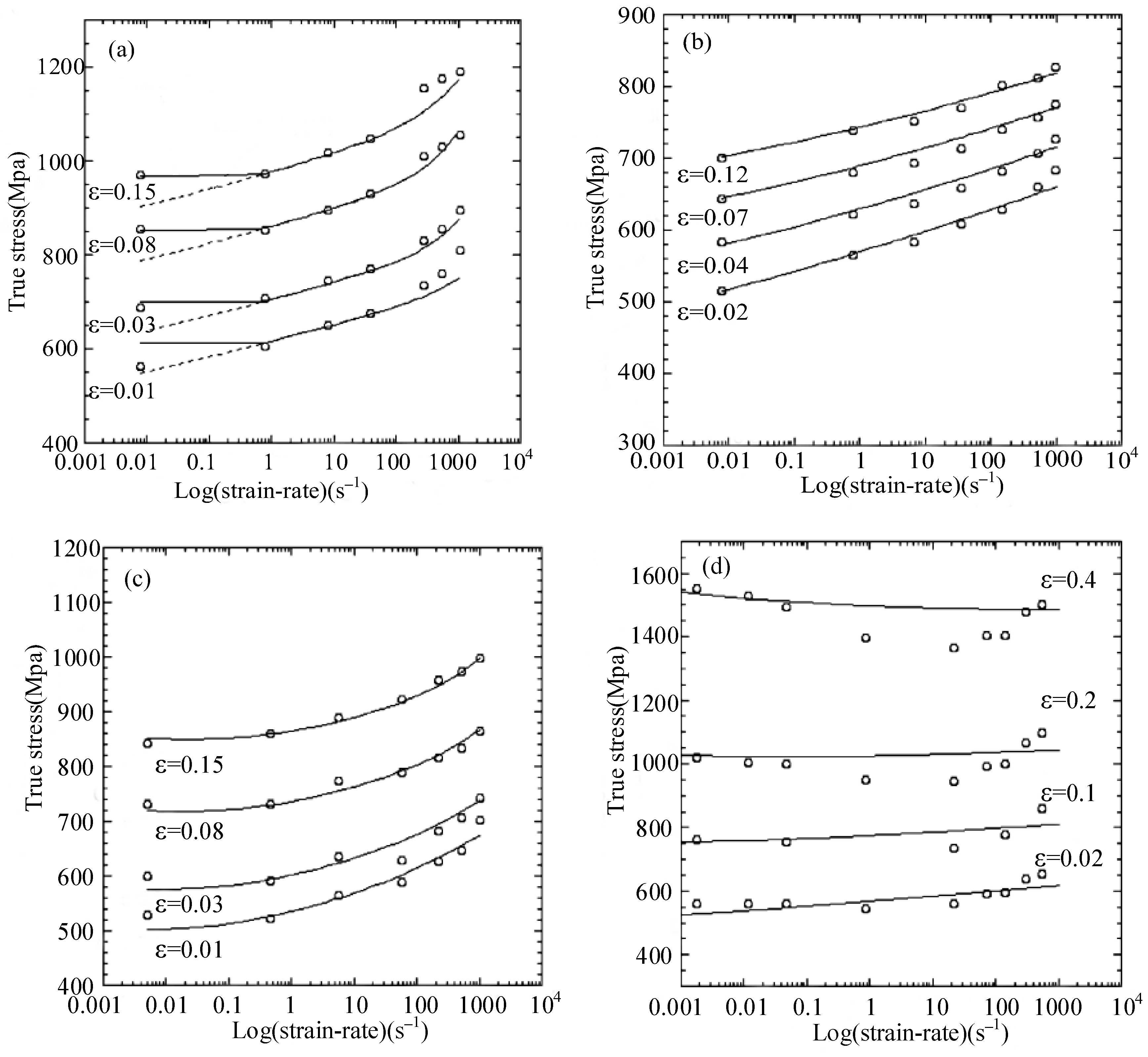
Yu et al. [17] used the KH model to describe the flow behavior of DP600 steel, as shown in Figure 4. The results show that the KH model can almost perfectly describe the correlation between the stress and plastic strain under the strain rate 10−4 s−1. However, the KH model neglects the coupling effect of strain and strain rate on work hardening, and does not consider the effect of temperature, so there is a large error between the predicted results of KH model and the measured results of mechanical properties of DP600 steel at high strain rate (600 s−1).
In view of the above shortcomings, Equation (12) is modified to better describe the effect of strain rate on flow stress:
σ = f ( ε p , ε ˙ p ) = σ 0 f ^ 2 ( ε ˙ p ) + E p a e α ε p
f ^ 2 ( ε ˙ p ) = 1 + D ln ( ε ˙ p ε ˙ 0 p ) m
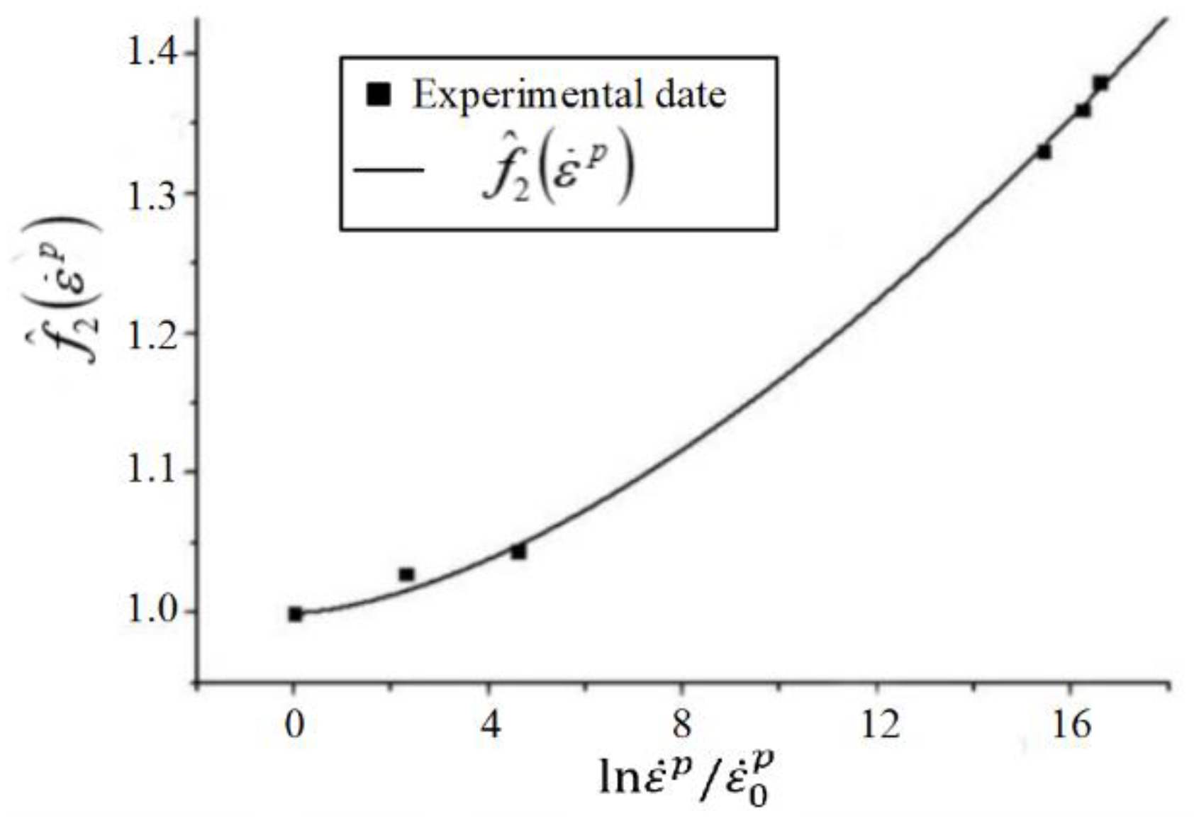
where σ is flow stress, ε p is plastic strain, ε ˙ p represents the current strain rate, ε ˙ 0 p is the reference strain rate, and m is the material constant. The relation curve between f ^ 2 ( ε ˙ p ) and dimensionless parameter ln ε ˙ p / ε ˙ 0 p is shown in Figure 5.
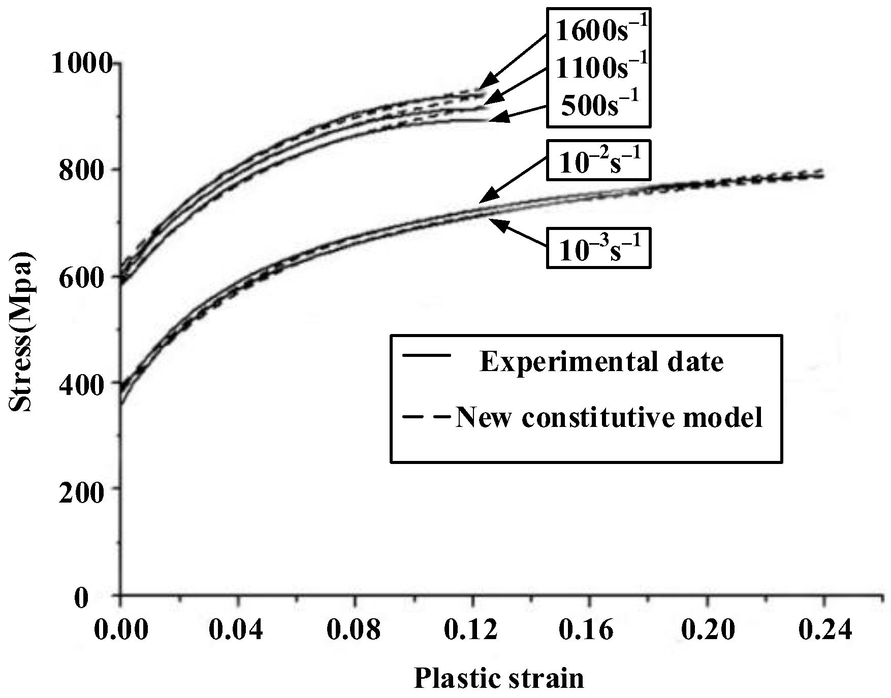
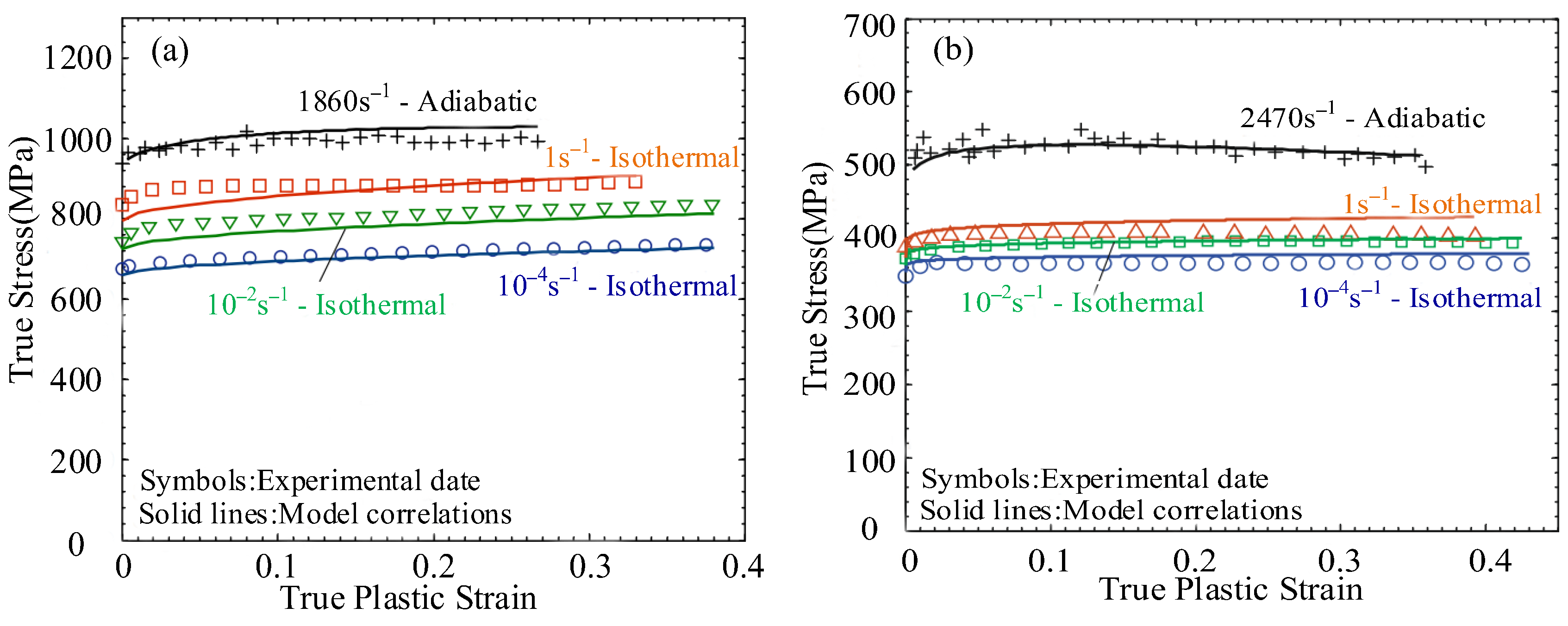
With the help of the modified model (Equations (15) and (16)), the rheological properties of DP600 steel were predicted at strain rates of 10−3 s−1, 10−2 s−1, 500 s−1, 1100 s−1, and 1600 s−1, respectively, and the predict results are shown in Figure 6. Compared with the experimental results, the modified KH model can better describe the deformation behavior of DP600 steel at a high strain rate.
Khan and Liang [18] modified the relationship between J 2 and D 2 P in the original KH model by considering the influence of temperature effect on the mechanical properties of materials, and established a new KHL constitutive model, as shown in Equation (18):
J 2 = f 1 ( ε 2 , D 2 p ) f 2 ( T )
σ = [ A + B ( 1 ln ε ˙ ln D 0 p ) n ε n 0 ] e c ln ε ˙ ( 1 T * m )
T * = T T r T m T r
where T is the absolute temperature. ε is equivalent plastic strain. f 1 ( ε 2 , D 2 p ) is a function characterizing the coupling effect of strain and strain rate on work hardening. Tr is the reference temperature. Tm is the melting temperature of the material, A, B, n, n0, and m are fitting parameters based on test data.
In 2000, Khan et al. [19] introduced the Hall–Petch relation into the KHL model, and replaced constant A (yield stress of material under reference strain rate) with the Hall–Petch relation. The modified KHL model comprehensively characterized the effects of grain size, work hardening, rate, and temperature on the plastic deformation behavior of materials. The modified KHL model was as follows:
σ = [ ( a + k d ) + B ( 1 ln ( ε ˙ p ) ln D 0 p ) n 1 ( ε p ) n 0 ] × ( ε ˙ p ε ˙ p ) c ( 1 T m )
σ y = a + k d
where σy is yield stress, d is the average grain size of polycrystalline, and a and k are material constants.
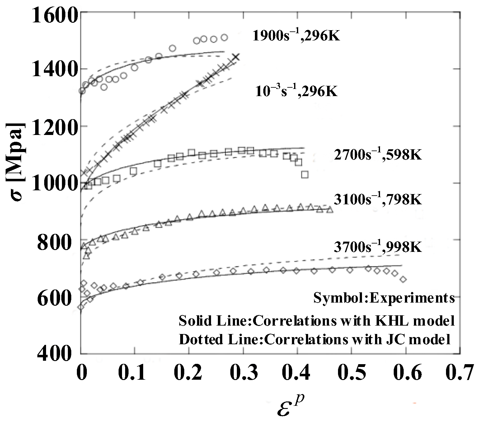
Khan et al. [20] used the modified KHL constitutive model (Equation (20)) compared with J–C model, as shown in Figure 7. The results show that the prediction accuracy of the modified KHL model for the rheologiacal characteristics of Ti-6AL-4V alloy is significantly higher than that of the J–C model.
However, when the deformation temperature of the constitutive Equation (20) is lower than the reference temperature, the temperature term ( 1 T * m ) will return to a negative value, which will make the model unable to predict the viscoplastic response of the material below room temperature. Therefore, in order to characterize the mechanical properties of metal materials at low temperature, Khan [20] revised Equation (20), and the modified flow stress model is shown as follows:
σ = ( a + k d ) [ 1 + B a ( 1 ln ( ε ˙ p ) ln D 0 p ) n 1 ( ε p ) n 0 ] × ( ε ˙ p ε ˙ p ) c ( T m T T m T r ) m
a + k d = { a 1 + k 1 d f o r 0 d 0.5 d 0.5 a 2 + k 2 d f o r d 0.5 d 0.5
where T is the absolute temperature, Tm is the melting temperature, Tr is the reference temperature, a and k are material constants, and can be determined from experiments at a strain rate of ε ˙ = 1 . d* is defined as the reference grain size when the yield stress begins to increase significantly. a 1 , a 2 , k 1 , and  k 2 are constants based on the yield stress and grain size (d0.5).
As the grain size of the material decreases to the nanometer range, the strain hardening behavior also increases. The modified constitutive Equation (22) is very close to the experimental results of nanocrystalline aluminum, as shown in Figure 8.
Based on the KHL model, Farrokh and Khan [21] established a new viscoplastic constitutive equation Khan–Liang–Farrokh (KLF) model (Equation (24)) related to grain size and temperature:
σ = [ ( a + k d n ) + B ( d d 0 ) n 2 ( ( 1 ln ( ε ˙ p ) ln ( D 0 p ) ) ( T m T ) ) ( ε P ) n o ] × ( ε ˙ p ε ˙ p ) c ( T m T T m T r )
where εp is plastic strain. ε ˙ p is the current strain rate. σ is the flow stress. Tm represents the melting temperature of the material. T is ambient temperature. Tr is the reference temperature. D 0 p is the optional upper limit strain rate. ε ˙ p * is the reference strain rate. n * is the material following the Hall–Petch relationship. d is the average size of grains. d0 is the grain size of coarse grains. a , k, B, no, n1, n2, c, and m are the material constants of the KHL model.
With the help of the above theoretical models, the uniaxial compressive deformation behavior of mechanically milled ultrafine grain and nanocrystalline Cu and Al under quasi-static and dynamic strain rates was investigated [21], as shown in Figure 9 and Figure 10. The KLF model can well capture the variation of yield stress and work hardening behavior with grain size (to large strain), and can respond to different grain sizes (from coarse grain to nanocrystalline materials), different strain rates (quasi-static to dynamic), and different temperatures (low temperature and high temperature).

2.3. Fields–Backofen (FB) Model

In 1957, Fields and Backofen [22] proposed the FB model for most metal materials:
σ = k ε n ε m
where k is the strength coefficient, n is the strain hardening index, and m is the strain rate sensitivity index.
The FB model is widely used to describe the stress–strain relationship, and can be used to express the work hardening phenomenon in the process of plastic deformation through the strain hardening index (n) and strain rate sensitive index (m).
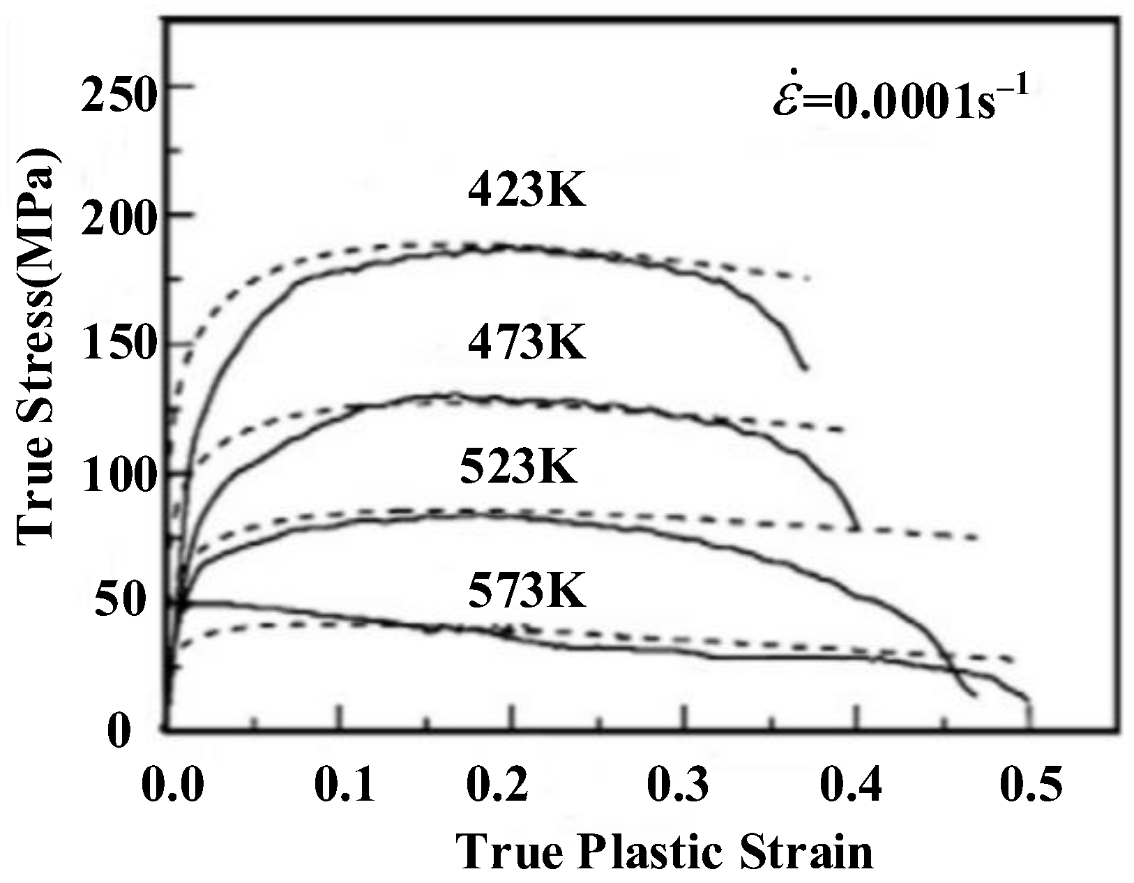
Based on the FB model, Cheng et al. [23] studied the uniaxial tensile deformation behavior of an AZ31 magnesium alloy sheet under strain rates of 0.1–0.0001 s−1 and deformation temperatures of 423–573 K, as shown in Figure 11. By comparing the predicted results of FB model with the experimental results, the predicted results are in good agreement with the experimental results at low temperature and high strain rate. However, the rheological deformation of AZ31 magnesium alloy sheet at higher temperature and lower strain rate shows obvious recrystallization softening characteristics; the FB model cannot characterize the softening behavior of the material.
In view of the inaccuracy of the softening description of the FB model, Zhang [24] and Chen [25] introduced a softening term into the FB model to characterize the softening behavior of materials in the process of plastic deformation, and modified the FB model on this basis. The modified FB model established is shown below:
σ = K ε n ε m exp ( b T + s ε )
s = dln σ d ε  
where K is the strength coefficient, n is the strain hardening index, m is the strain rate sensitivity index, b is material constant, and T is the absolute temperature. s represents the softening ratio of magnesium alloy with increasing of the strain.
The modified magnesium model was used to predict the deformation behavior of AZ31 magnesium alloy [23], as shown in Figure 12. The results showed that the modified FB model could better characterize the softening behavior of the material during plastic deformation.

2.4. Hansel–Spittel Model

In 1978, Hansel and Spittel [26] combined the classical strain rate power-law model with the Hollomon and Swift model, treating the corresponding material constants as functions of strain and temperature. Based on this, a new equation of thermal deformation flow stress is proposed:
σ = A e m 1 T ε m 2 ε ˙ m 3 e m 4 / ε ( 1 + ε ) m 5 T e m 6 ε ε ˙ m 7 T T m 8
where A is the stress intensity coefficient, m1 is the temperature-dependent coefficient, m2 is the strain strengthening coefficient, m3 is the strengthening coefficient of strain rate, m4 is the strain softening coefficient, m5 is the temperature-dependent strain strengthening coefficient, m6 is strain correlation coefficient, m7 is the strengthening coefficient of strain rate related to temperature, and m8 is the temperature coefficient.
Due to the numerous parameters of the Hansel–Spittel model, it is very difficult for regression analysis. Therefore, Spigarelli and El Mehtedi [27] modified Equation (28) to reduce the regression coefficient and make it have better prediction ability:
sinh ( α σ ) = A e m 1 T ε m 2 ε m 3 e m 4 / ε ( 1 + ε ) m 5 T e m 6 ε
Under thermal deformation conditions, the strain rate sensitivity of material flow stress decreases with the increase of strain. However, the Hansel–Spittel model is not sufficient to describe the change of strain rate sensitivity under given temperature and strain conditions; Brown proposed a modified Hansel–Spittel model (Equations (30)–(32)) to describe the strain rate sensitivity more accurately [28]. In the Brown modified model, the stress component is assumed to be temperature-independent under a given strain (or steady state) condition; thus, the parameters m7 and m8 were neglected to simplify the constitutive model:
sinh ( α σ ) = A e m 1 T ε m 2 ε ˙ m 3 e m 4 / ε ( 1 + ε ) m 5 T e m 6 ε
ε ˙ exp ( Q R T ) = A 1 σ , f o r α σ < 0.8
ε ˙ exp ( Q R T ) = A 2 exp ( β σ ) , f o r α σ < 0.8
where σ is the flow stress, T is the absolute temperature, A, A2, and β are the material constant, n is the strain rate sensitive index, R is the molar constant of gas R = 8.31 J/mol·K, α is the stress level parameter, and Q is the activation energy of the material.
The results show that the modified Hansel–Spittel model can better characterize the rheological properties of CoCrFeMnNi alloy than the original Hansel–Spittel model, as shown in Figure 13, where the real lines represent simulated data, and the virtual lines represent experimental data.

2.5. Arrhenius Model

The Arrhenius equation is widely used to describe the relationship between flow stress and strain rate and deformation temperature under high temperature deformation conditions. In the exponential equation, the Zener–Hollomon parameter is used to represent the influence of temperature and strain rate on the deformation behavior. Moreover, a more accurate approximation between the Zener–Hollomon parameter and the flow stress is obtained by hyperbolic function. The Arrhenius constitutive equation is as follows [29]:
ε ˙ = { A 1 σ n 1 , α σ < 0.8 A 2 exp ( β σ ) , α σ < 1.2 A [ sinh ( α σ ) ] n exp [ Q / ( R T ) ] , f o r   a l l   σ
where A1, A2, A, n1, n, α and β are material constants, Q is the activation energy of deformation ( K J / m o l ), R is a general gas constant ( 8.31   J / ( m o l K ) ), σ is flow stress. The relationship between α, β and n1 can be expressed as α = β / n 1 .
According to the definition of hyperbolic function, the flow stress σ can be written as a function of Z parameter:
σ = 1 α ln { ( Z A ) 1 / n + [ ( Z A ) 2 / n + 1 ] 1 / 2 }
In recent years, many scholars [30,31] have determined the flow stress of different metals and alloys during thermal deformation by the Arrhenius model. Since the Arrhenius model does not consider the influence of strain on flow stress, the prediction accuracy of this model is not high under large deformation conditions. By constructing the polynomial relationship between the model parameters Q, A, N, and α and the strain, respectively. The modified Zener-Hollomon model coupled with the influence of temperature, strain rate, and deformation was established [32], as shown in Equations (35) and (36):
{ Q = B 0 + B 1 ε + B 2 ε 2 + B 3 ε 3 + B 4 ε 4 + B 5 ε 5 n = D 0 + D 1 ε + D 2 ε 2 + D 3 ε 3 + D 4 ε 4 + D 5 ε 5 I n A = E 0 + E 1 ε + E 2 ε 2 + E 3 ε 3 + E 4 ε 4 + E 5 ε 5 α = F 0 + F 1 ε + F 2 ε 2 + F 3 ε 3 + F 4 ε 4 + F 5 ε 5
Z = ε ˙ 4 / 3 exp ( Q R T )
ln Z = ln Z + 1 3 ln ε ˙
σ = 1 α ln { ( Z A ) 1 / n + [ ( Z A ) 2 / n + 1 ] 1 / 2 }

2.6. Molinari–Ravichandran Model

In 2005, Molinari and Ravichandran proposed a phenomenological constitutive model (MR model) that can describe the flow behavior of metals under various loading conditions [33,34]. The MR model is based on a single internal variable δ, which is related to the characteristic length of the microstructure formed during metal deformation. The flow stress σ is expressed as a function of the inherent resistance σ ^ 0 and strain rate ε ˙ of the material:
σ = σ 0 ( ε ˙ ε ˙ 0 ) 1 m
σ ^ 0 = σ ^ ( d ) ( δ 0 δ )
where ε ˙ 0 is the reference strain rate, d is the average grain size, and m represents the parameter of instantaneous strain rate sensitivity dependent on temperature. The reduction of the internal characteristic length δ with an increase of increasing equivalent plastic strain ε, which can be expressed by the following phenomenological evolution equation:
d δ d ε = δ r δ s [ δ 2 δ s δ ]
where δr is a dimensionless parameter characterizing the refinement rate of microstructure. δs is the saturation length at relatively large strains, which both can be a function of strain rate and temperature.
Assume δr and δs are constants, which is the case for constant strain rate and temperature. Equation (41) can be expressed as follows:
δ s δ = [ 1 { 1 δ s δ 0 } exp ( δ r ε ) ]
where δ0 is the initial internal characteristic length. However, when the saturation of the “microstructural length” reaches the limiting value δs, the flow stress will also be induced to reach saturation values.
The laws proposed for δr and δs can be based on the theory of thermally activated processes or on empirical relations depending on temperature and strain rate:
δ r = δ r 0 [ 1 + a r ( ε ˙ ε ˙ r 0 ) ξ r ( T T 0 ) v r ]
δ s = δ s 0 [ 1 a s ( ε ˙ ε ˙ s 0 ) ξ s ( T T 0 ) v s ]
where δs and δs0 are the saturation values of effective microstructure length δ and the reference values at zero strain rate, respectively. The material constants αs, ξs, and vs control the strain rate and the dependence of δs on temperature; similarly, δr depends on δr0, αr, ξr, and vr.
In order to avoid negative values of the MR model at relatively low strain rates, Molinari and Durrenberger [35] proposed a new phenomenological model (DMR model). The flow stress is defined as the sum of the internal stress representing the long-term interaction and the thermally activated effective stress:
σ t h = { σ r e f [ a b T ln ( ε ˙ 0 ε ˙ ) ] 1 / m , a b T ln ( ε ˙ 0 ε ˙ ) 0 0 , a b T ln ( ε ˙ 0 ε ˙ ) 0
In the isothermal condition, Durrenberger [35] pointed out that Equation (45) can be simplified as
σ t h = σ r e f ( T 0 T ) v [ a b ln ( ε ˙ 0 ε ˙ ) ] 1 / m
where σref is a reference stress, T0 is the reference temperature, ε ˙ 0 is the reference strain-rate, ν* is the temperature sensitivity, a and b are material constants, and m characterizes the instantaneous rate sensitivity.
The DMR model is considered to be able to accurately describe the thermal and viscoplastic response behavior of metals under harsh loading conditions [36]. Based on the DMR model, the strain rate sensitivity simulation and experimental data of four kinds of sheets for automobile forming are compared as shown in Figure 14 (Circle points represent experimental data, real lines represent simulation data) [36]. It can be seen that the DMR model can effectively describe the strain hardening effect of materials under different strain plastic rates.

2.7. Comparison and Analysis of Phenomenological Models

In addition to the above widely used models, there are many phenomenological constitutive models. Due to the limitation of the length of the paper, other phenomenological constitutive models are not introduced in detail in this paper.
In order to facilitate readers to understand the features and applicable conditions of the phenomenological constitutive model introduced in the article, the main features of each model are summarized in Table 1.

3. Constitutive Model Based on Microscopic Characteristics

The phenomenological model can obtain the corresponding model parameters through the fitting and the regression analysis of experimental data, which makes the process of solving the model easy. However, under the extreme deformation conditions, such as large deformation and high temperature, the phenomenological model cannot characterize the effect of the change of microstructure on the macroscopic mechanical properties of materials [37].
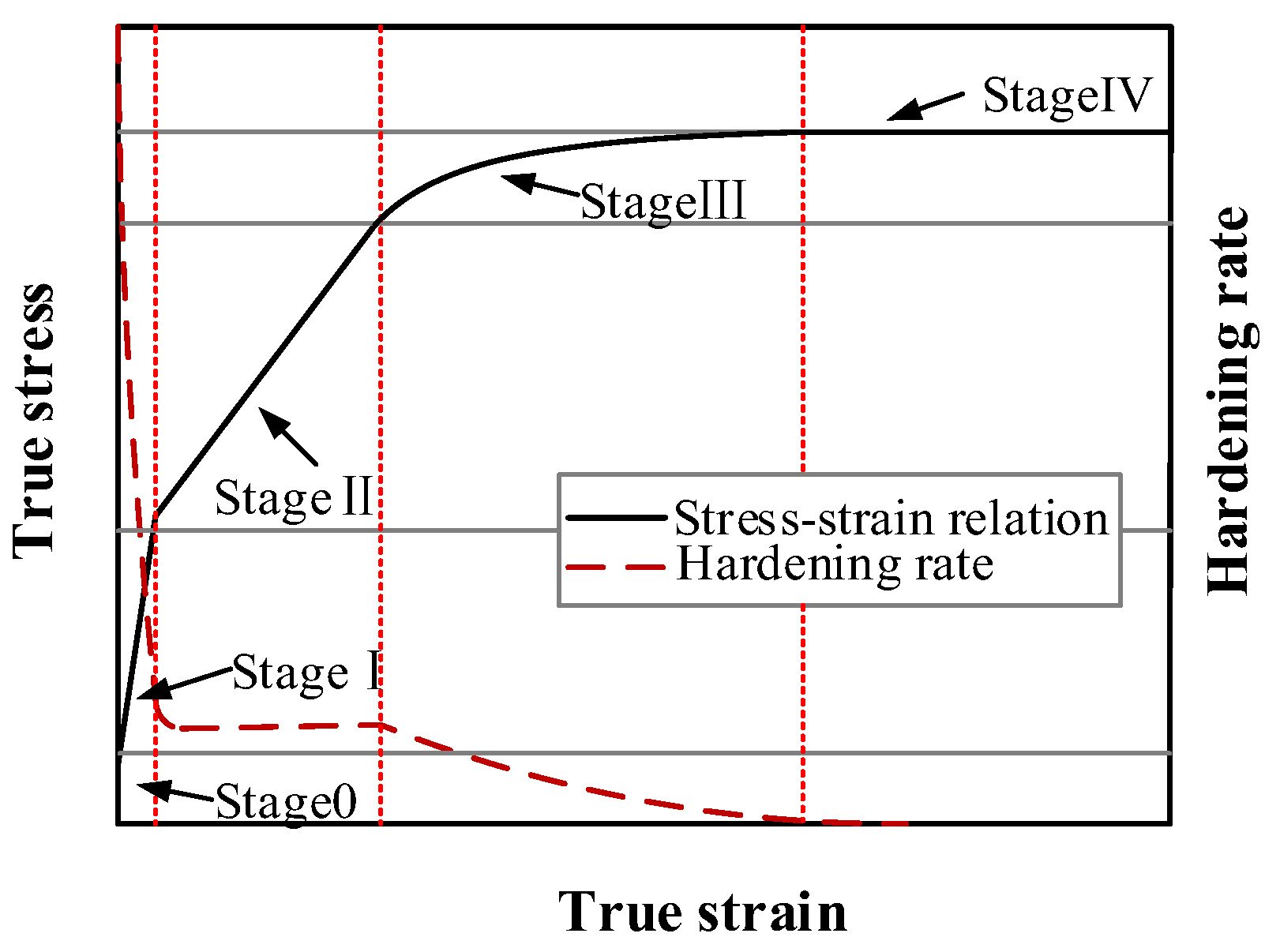
In the thermal deformation process, the plastic deformation behavior of the material can be divided into four stages, as shown in Figure 15. In the first deformation stage (stage 1), the accumulation and multiplication of dislocations are the main reasons for material hardening. However, in the second stage of deformation (stage 2), the temperature effect and strain hardening simultaneously affect the flow stress of the material. In this stage, the strain hardening effect plays a leading role, and the strain hardening rate of the material gradually decreases due to the effect of temperature effect. In the third stage of deformation (stage 3), with the increase of deformation amount, dislocations accumulate continuously and grain boundary energy storage increases, which enhances dynamic recrystallization (DRV) under temperature and reduces strain hardening effect. In the fourth stage (stage 4), strain hardening, dynamic recovery, and dynamic re-crystallization are relatively balanced, and the flow stress of the material is in the steady state deformation stage.
Based on the above micro deformation theory, He [38] believed that the total strain rate ε ˙ in isothermal deformation was composed of elastic strain rate ε ˙ e   and inelastic part ε ˙ i n , and proposed a multi-scale constitutive model based on dislocation density to describe the thermal deformation behavior of HEAs materials. As shown in Equations (47) and (48):
ε ˙ = ε ˙ e + ε ˙ i n
ε ˙ i n = ρ c m b λ v a m exp ( Δ G k T ) 3 2 σ e q S
where ρ c m is the dislocation density, b is magnitude of the Burgers vector, λ is the average distance, v a denotes the attempt frequency, m is the Taylor orientation factor, Δ G is the activation energy, k is the Boltzmann constant, T is the absolute temperature, σ e q is the equivalent stress, and S is the deviatoric part of local stress tensor.

3.1. Zerilli–Armstrong Model (ZA Model)

The ZA model takes into account the effects of strain hardening, strain rate hardening, and temperature softening on the plastic deformation behavior of metals and alloys, and is one of the most widely used dislocation density models. The ZA model divides the flow stress into thermal component and athermal component, as shown in Equation (49) [39]:
σ = σ a + σ t h
The athermal component σa considering the effect of grain size is expressed as
σ a = C 0 + k l 1 / 2
where l is the average grain size, k is the Hall–Petch constant, C0 is the fitting parameter.
The thermal stress component σth can be calculated by Equations (51) and (52):
σ t h = M Δ G 0 A b e β T
β = C 3 + C 4 ln ε ˙
where M is the direction factor, ΔG0 is the free energy of thermal activation at an absolute temperature of zero, A is the thermal activation area at at an absolute temperature of zero, b is the Burgers vector, β is a parameter related to strain rate. For BCC materials, A is a constant, that is, the deformation activation energy of BCC material is not affected by plastic strain. For FCC materials, the relationship between A and plastic strain can be expressed as ε 1 / 2 .
Therefore, according to the Equations (50)–(52), the constitutive equation of Z-A model can be expressed as
σ = C 0 + C 1 exp ( C 3 T + C 4 T ln ε ˙ ) + C 5 ε n   ,   for   BCC   materials
σ = C 0 + C 2 ε 1 2 exp ( C 3 T + C 4 T ln ε ˙ ) ,   for   FCC   materials
where C0, C1, C2, C3, C4, C5, and n are fitting parameters. It can be seen from Equations (53) and (54) that the strain hardening index is affected by strain rate and temperature for FCC materials, while for BCC materials, the strain hardening index is constant.
The ZA constitutive model does not fully realize the coupling effect of temperature, strain, and strain rate. Therefore, some improved ZA models have been proposed in recent years. Zhang et al. [40] proposed an improved flow stress model of IC10 alloy considering the effects of temperature, strain rate, and strain on the flow behavior of IC10 alloy under a wide range of temperature and strain rate deformation conditions, as shown in Equations (55) and (56). Moreover, the flow behavior of IC10 under different deformation conditions is predicted by the modified model, and the prediction results are shown in Figure 16. The results show that the modified ZA model can predict the rheological behavior of metal materials more accurately:
σ = C 0 + C 1 exp [ ( C 3 T + C 4 T ln ( ε ˙ r ( ε ) r ( ε ˙ ) ) ) f ( T ) ] + C ε 5 n ,   for   BCC   materials
σ = C 0 + C 2 ε 1 2 exp [ ( C 3 T + C 4 T ln ( ε ˙ r ( ε ) r ( ε ˙ ) ) ) f ( T ) ] ,   for   FCC   materials
r ( ε ) = ρ 0 + M ε
where ρ0 is the initial dislocation density of materials. M is the material constant related to the increase rate of dislocation density. C0, C1, C2, C”3, C’4, and n are fitting parameters.
In order to better characterize the flow stress of D9 alloy under the high temperature, based on the J–C model, Samantaray [41] modified the ZA model (Equation (54)) by considering the coupling effect of temperature, strain, strain rate, and temperature on flow stress. The modified model proposed by Samantaray is shown in Equation (58), and the predicted results of D9 alloy are shown in Figure 17:
σ = ( C 1 + C 2 ε n ) exp { ( C 3 + C 4 ε ) ( T T r ) + ( C 5 + C 6 ( T T r ) ) ln ( ε ˙ / ε ˙ r ) }
where ε ˙ r   and T r are the reference strain rate and the reference temperature, respectively. C1, C2, C3, C4, C5, C6, and n are all material constants, and they can be obtained by fitting experimental data.

3.2. Preston–Tonks–Wallace (PTW) Model

In 2003, Preston et al. [42] proposed a numerical simulation model of metal plastic flow suitable for explosive load and high-speed impact. At low strain rate, the dependence of plastic strain rate on applied stress is in the form of Arrhenius, but the activation energy is singular at zero stress, so the deformation rate disappears at this limit. The work hardening effect is modeled as a generalized Voce law. The constitutive model of the low strain rate region can be expressed as
τ ^ = τ ^ s + 1 p ( s 0 τ ^ y ) ln { 1 { 1 exp ( p τ ^ s τ ^ s τ ^ y s 0 τ ^ y ) exp [ p θ ψ ( s 0 τ ^ y ) ( exp ( p τ ^ s τ ^ y s 0 τ ^ y ) 1 ) ] } }
where ψ is the plastic strain, p is a dimensionless material parameter, and θ is determined by the slope of work hardening data. τ ^ is the normalized flow stress. τ ^ s is the work hardening saturated stress under thermal activation condition,   τ ^ y is the yield stress,
τ ^ s = s 0 ( s 0 s ) e r f [ k T ^ ln ( γ ξ ˙ ψ ˙ ) ]
τ ^ y = y 0 ( y 0 y ) e r f [ k T ^ ln ( γ ξ ˙ ψ ˙ ) ]
where Ψ ˙ is the plastic strain rate. s0 and s are the values of τ ^ s when temperature is zero and infinite, respectively. y0 and y are the values of   τ ^ y when temperature is zero and infinite, respectively. k and γ are dimensionless material constants. T ^ = T / T m (T is deformation temperature, Tm is melting temperature). ξ ˙ is the equivalent scaling factor, and it can be defined as
ξ ˙ = 1 2 ( 4 π ρ 3 M ) 1 3 ( G ρ ) 1 2
where ρ is material density, M is atomic mass, G is the shear modulus of material, which is the function of density and temperature, G = G 0 ( 1 α T ^ ) , where G0 is the shear modulus at absolute temperature, and α is the temperature dependence coefficient.
Under ultra-high strain rate loading under strong shock wave, the relationship between plastic strain rate and critical shear stress satisfies an exponential function, and the yield stress is equal to the saturation stress. Therefore, the model can be expressed as follows:
τ ^ s = τ ^ y = A ( ξ ˙ ψ ˙ ) β
where A and β are the material constants.
In order to maintain the continuity of the model, the saturation stress and yield stress in the transition zone from the low-strain rate region to the high-strain rate region are expressed as
τ ^ s = max { s 0 ( s 0 s ) e r f [ k T ^ ln ( γ ξ ˙ ψ ˙ ) ] , s 0 ( ψ ˙ γ ξ ˙ ) β }
τ ^ y = max { y 0 ( y 0 y ) e r f [ k T ^ ln ( γ ξ ˙ ψ ˙ ) ] , min [ y 1 ( ψ ˙ γ ξ ˙ ) y 2 , s o ( ψ ˙ γ ξ ˙ ) β ]
In order to explain the strain hardening at 0–106 s−1 strain rate, Kim [43] used the Voce equation to modify the strain hardening term in the original PTW model, and the modified constitutive equation is shown in Equations (66) and (67). Compared with the other constitutive models, the Kim’s modified PTW model can better describe the deformation behavior of tantalum in a wider strain, strain rate, and temperature range, as shown in Figure 18.
τ ^ = τ ^ y + A e C log ε ¯ ˙ ( 1 e B ε ¯ )
where τ ^ is the initial yield stress, and it can be expressed as
τ ^ y = max { y 0 ( y 0 y ) e r f [ k T ^ ln ( γ ξ ˙ ε ¯ ˙ ) ] , y 0 ( ε ¯ ˙ γ ξ ˙ ) β }
where A, B, and C are material constants. A represents the maximum strain hardening at unit strain rate, B represents the saturation velocity of control hardening, and C represents the dependence of maximum hardening on strain rate.

3.3. Rusinek–Klepaczko (RK) Model

Considering the influence of strain hardening, strain rate sensitivity, temperature effect and other factors on the material deformation process, Rusinek and Klepaczko [44] proposed a viscoplastic constitutive model (RK model), which decomposed the flow stress σ ¯ into the sum of internal stress σu and effective stress σ*:
σ ¯ ( ε ¯ p , ε ¯ ˙ p , T ) = E ( T ) E 0 [ σ u ( ε ¯ p , ε ¯ ˙ p , T ) + σ ( ε ¯ ˙ p , T ) ]
E ( T ) = E 0 { 1 T T m exp [ θ ( 1 T m T ) ] }
where E0, Tm, and θ* represent the elastic modulus, melting point temperature, and characteristic assimilation temperature of the material at absolute zero, respectively.
The internal stress σu can be expressed as
σ ¯ u ( ε ¯ p , ε ¯ ˙ p , T ) = B ( ε ¯ ˙ p , T ) ( ε 0 + ε ¯ p ) n ( ε ¯ ˙ p , T )
B ( ε ¯ ˙ p , T ) = B 0 [ T T m log ( ε ˙ max ε ¯ ˙ p ) ] v
n ( ε ¯ ˙ , T ) = n 0 [ 1 D 2 T T m log ( ε ¯ ˙ p ε ˙ min ) ]
where B0 and D2 are material parameters. v is the temperature sensitive coefficient. n0 is the strain hardening index at absolute zero. ε ˙ m i n   and ε ˙ m a x   are the minimum strain and maximum strain rate accepted by material, respectively.
The effective stress can be obtained according to the Arrhenius equation, as shown in Equation (73):
σ ( ε ¯ ˙ , T ) = σ 0 ( 1 D 1 ( T T m ) log ( ε ˙ max ε ¯ ˙ p ) ) m
In the effective stress equation, σ* is the effective stress at absolute zero. D1 is the material parameters. m* is a constant allowing the definition of strain rate and temperature dependence.
Aiming at the problem that the original RK model cannot accurately describe the viscoplastic behavior of aluminum alloy, Rusinek et al. [45] modified the RK model. They defined the macroscopic negative strain rate sensitivity (NSRS) and viscous resistance, and added a negative strain rate sensitivity term on the basis of the original RK model, as shown in Equation (74):
σ ¯ = ( ε ¯ p , ε ¯ ˙ p , T ) = E ( T ) E 0 [ σ μ ( ε ¯ p , ε ¯ ˙ p , T ) + σ ( ε ¯ ˙ , T ) + σ n s ( ε ¯ ˙ p , T ) ]
where σ n s ( ε - ˙ p , T ) is the stress component of NSRS, which depends on the strain rate and temperature:
σ n s ( ε ¯ ˙ p , T ) = σ 0 n s log ( ε ˙ t r a n s ε ¯ ˙ p ) [ 1 D 3 ( T m T ) log ( ε ¯ ˙ p ε ˙ max ) ]
In the above formula, σ 0 n s and D3 are material parameters, which describe the stress drop caused by the interaction of dynamic strain aging (DSA) with strain rate and temperature, respectively. ε ˙ t r a n s is the turning point from positive to negative strain rate sensitivity, which can be obtained by fitting experimental results.
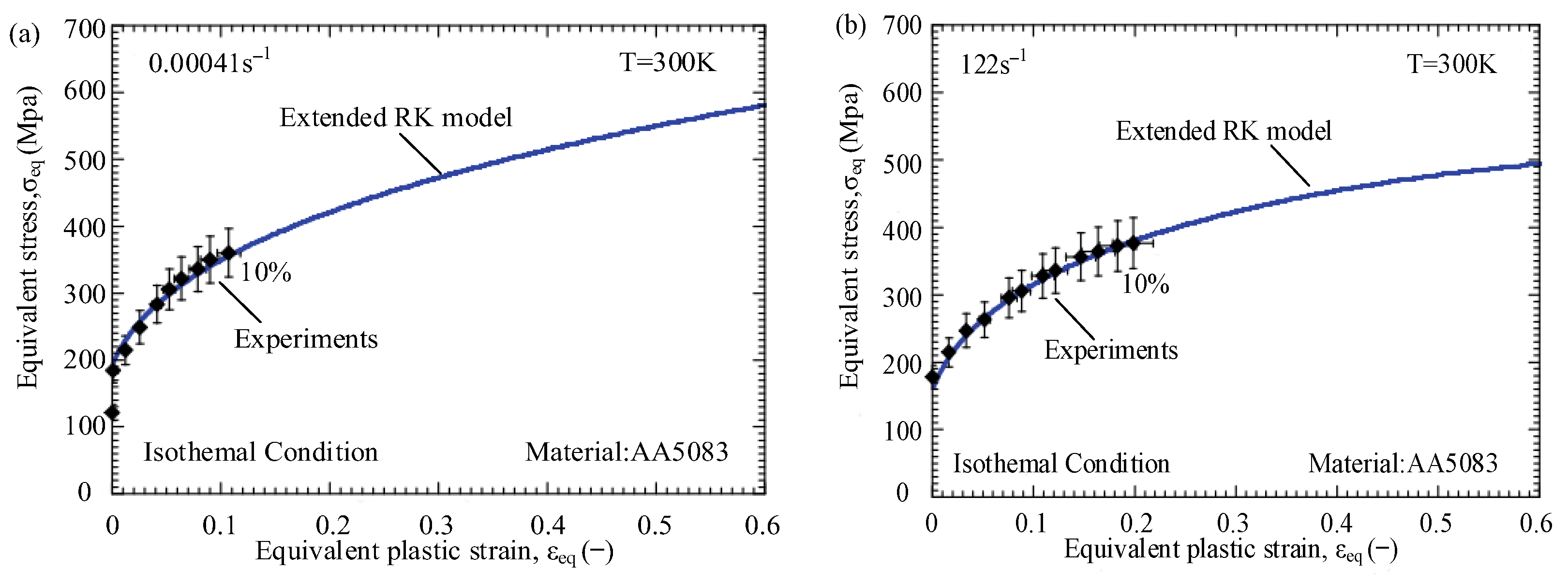
Based on the Equations (74) and (75), the viscoplastic behavior of AA5083 aluminum alloy was researched, as shown in Figure 19 and Figure 20. It can be seen that the analytical prediction results are consistent with the experimental results under different strain rates, and the results also prove that the effectiveness of the model is describing correctly the DSA effect [45].
Another extension of the RK model is by adding a viscosity component related to the strain rate on the basis of the the equivalent Huber–Misses stress σ ¯ of the original model. In this way, the viscous resistance effect of face-centered cubic metal at high deformation rate is characterized. As shown in Equation (76),
σ ¯ ( ε ¯ p , ε ¯ ˙ p , T ) = E ( T ) E 0 [ σ μ ( ε ¯ p , ε ¯ ˙ p , T ) + σ ( ε ¯ ˙ p , T ) ] + σ a t h ( ε ¯ ˙ p )
where σ a t h ( ε - ˙ p ) is the stress component accounting for the viscous resistance which is just dependent on strain rate. σ a t h ( ε - ˙ p ) can be specifically expressed as
σ a t h ( ε ¯ ˙ p ) = χ [ 1 exp ( α ε ¯ ˙ p ) ]
α = M 2 B ρ m b 2 τ y
where M is the Taylor factor, B is the resistance coefficient, ρm is the mobile dislocation density, and b is the magnitude of the Burgers vector, χ is a material constant, α represents an effective damping coefficient affecting the dislocation motion, and τy denotes the effective damping coefficient that affects the dislocation motion.
In 2010, Rusinek et al. [10] proposed a modified RK model based on physical concepts. Compared with the original RK model, the internal stress σu is defined as a constant Y in the new model, and the effect of plastic strain is considered in the effective stress component σ*:
σ ¯ ( ε ¯ p , ε ¯ ˙ p , T ) = E ( T ) E 0 [ σ μ + σ ] + σ v s
where E(T) is an expression for the temperature-dependent Young’s modulus, as shown in Equation (80). E0, Tm, and θ * are Young’s modulus, melting point temperature, and characteristic assimilation temperature of the material at absolute zero, respectively. σ μ the internal stress of the material, in Equation (79), and the internal stress σ μ is equal to the flow stress Y of the materials without deformation, namely σ μ = Y . σ* is effective stress of the material, and the expression is shown in Equation (81). σ v s is the viscous stress component, and its expression as shown in Equation (82):
E ( T ) = E 0 { 1 T T m exp [ θ * ( 1 T m T ) ] } , T > 0
where Tm and θ * are melting point temperature and characteristic assimilation temperature of the material at absolute zero, respectively:
σ ( ε ¯ p , ε ¯ ˙ p , T ) = B ( ε ¯ p ) n [ 1 ξ 1 ( T T m ) log ( ε ˙ max ε ¯ ˙ p ) ] 1 ξ 2
where ξ1 and ξ2 are material constants describing temperature and rate sensitivities of the material, respectively. ε ˙ m a x the maximum strain-rate level for material:
σ v s ( ε ¯ ˙ p ) = χ [ 1 exp ( M 2 B ρ m b 2 τ y ε ¯ ˙ p ) ]

3.4. Cellular Automaton (CA) Model

In the dynamic re-crystallization (DRX) process, the accuracy of nucleation parameters is the key factor to simulate the micro-structure evolution. Goetz et al. [46] proposed the cellular automaton model (CA model) to describe the microstructure evolution during dynamic recrystallization. With plastic deformation, dislocation density evolution can be expressed by the following equation:
d ρ d ε = k 1 ρ k 2 ρ
where k1 and k2 are model parameters representing strain hardening and dynamic recovery, respectively. When the dislocation density exceeds the critical value ρc of DRX nucleation, a new atomic nucleus is formed on the grain boundary. For two-dimensional cellular automaton model, I(ρ>ρc) is defined as the number of nuclei formed per unit time. For boundary cells with dislocation density exceeding the critical value, the nucleation probability PN in the time step Δ t   i s
P N = I Δ t N C A
N C A = 1 L C A
where NCA is the number of cells along the unit boundary length. LCA is cell length.
Transformation probability PG can be expressed as
P G = v i Δ t L C A
In order to ensure that PN and PG are less than 1, an upper limit of Δt must be set. Therefore, the upper limit of Δt can be defined as the ratio of cell size LCA to the maximum growth rate vmax, namely,
Δ t = L C A v max = k 2 2 L C A m τ k 1 2
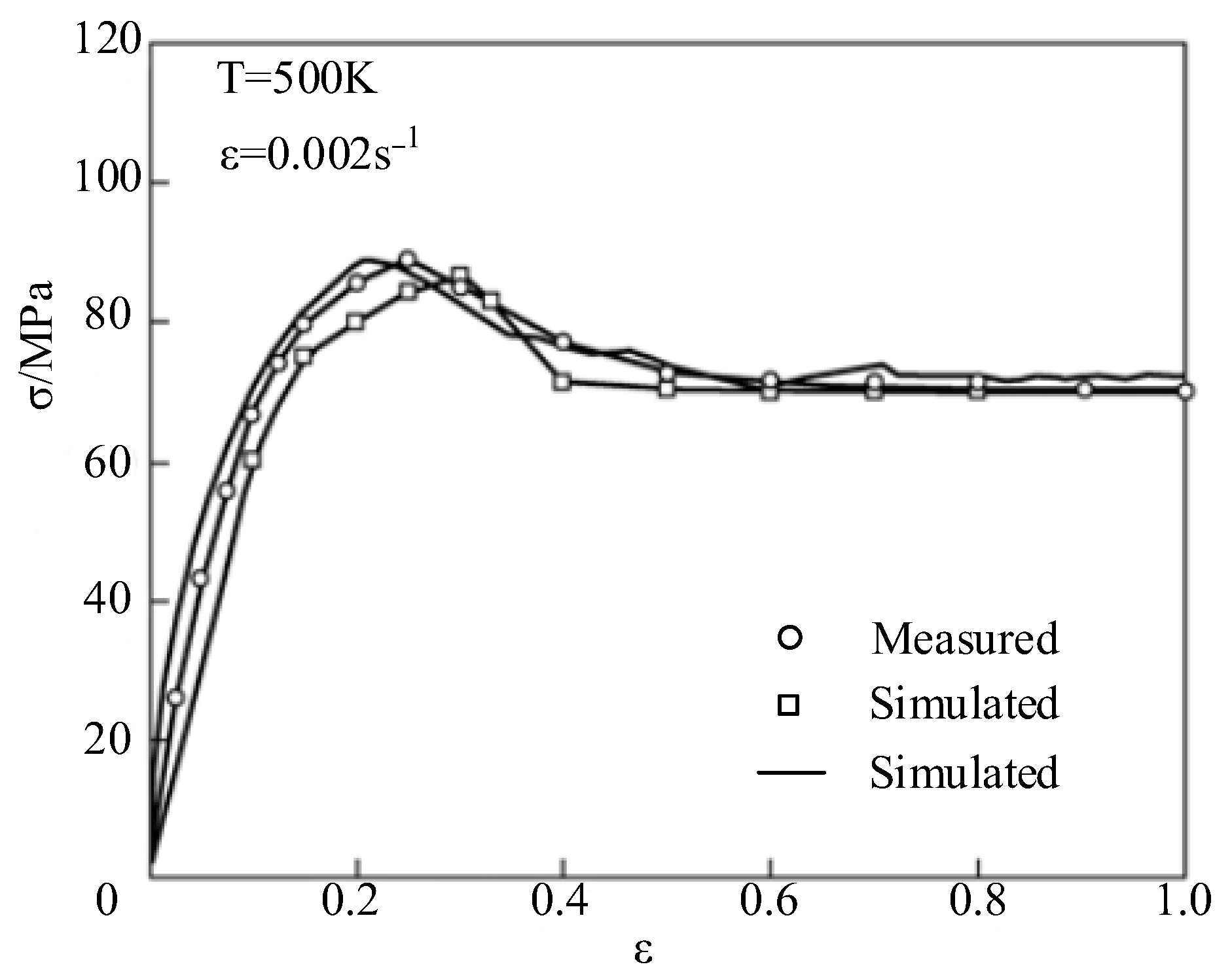
The study of dynamic re-crystallization behavior by CA method is 1 based on the physical metallurgical principles. However, it is difficult to accurately estimate the nucleation rate due to the complexity of DRX and limitation of experiments. The method proposed in the literature [47,48,49,50,51] can be used to identify the value of model parameters and explore their correlation with thermomechanical process parameters, which will contribute to the development of thermomechanical process analysis model. With the help of the new model parameter prediction method, Jin et al. [47] studied the microstructure evolution and flow stress behavior of oxygen-free high-conductivity (OFHC) copper during DRX at the temperature of 775 K and the strain rate of 0.002 s−1; the results are shown in Figure 21.

3.5. Steinberg–Guinan (SG) Model and Steinberg–Lund (SL) Model

Although the influence of strain rate has been taken into account for most constitutive models, the constitutive models mentioned above cannot accurately reflect the deformation behavior of materials under high strain rate conditions, such as impact and explosion. In order to accurately describe the deformation characteristics of materials under high strain rate and high-pressure coupling. Steinberg et al. [52] proposed the SG constitutive model in 1980. In the SG model, the shear modulus G and yield stress Y of the material are expressed as functions of pressure P and temperature T:
G = G 0 [ 1 + ( G P G 0 ) P η 1 / 3 + ( T 300 ) G T G 0 ]
Y = Y 0 [ 1 + β ( ε + ε i ) ] n [ 1 + ( Y P Y 0 ) P η 1 / 3 + ( T 300 ) G T G 0 ]
The SG model needs to satisfy Equations (90) and (91):
Y 0 [ 1 + β ( ε + ε i ) ] n Y max
G = Y = 0 ,   T T m
where G0 and Y0 are shear modulus and yield stress at temperature T = 300 K, presser P = 0 and strain ε = 0, respectively. η is the volume compression ratio of the material during deformation, η=V0/V. G’P is the first partial derivative of shear modulus G with respect to pressure P, G’T is the first partial derivative of shear modulus G with respect to temperature T, Y’P is the first partial derivative of yield stress Y with respect to pressure P. β and n are strain hardening parameters. Ymax is the maximum allowable value of material flow stress Y during strain hardening. εi is the initial strain, usually εi = 0. εi is the plastic strain of the material.
Under the condition of high-speed impact, Steinberg believed that the softening effect caused by the increase of temperature counteracts the hardening effect caused by the strain rate. When the strain rate is greater than 105 s−1, the flow stress of the material reaches the maximum value. Therefore, the expression of SG model has nothing to do with strain rate and cannot characterize the mechanical properties of materials at low strain rate. To overcome this shortcoming, Steinberg and Lund [53] introduced the calculation method of strain rate in the HM model into the SG model and established the Steinberg–Lund model (SL model), which decomposed the yield stress Y into thermal stress component YT and non-thermal stress component YA:
Y = [ Y T ( ε ˙ p , T ) + Y A f ( ε p ) ] G ( P , T ) G 0
where Y T ( ε ˙ p , T ) is the thermally activated part of the yield strength and is a function of ε ˙ p and T. Y A f ( ε p ) is the non-thermal part of the flow stress, f ( ε p ) = Y 0 [ 1 + β ( ε + ε i ) ] n . G(P, T) is the shear modulus associated with temperature T and pressure P:
ε ˙ p = { 1 C 1 exp [ 2 U K K T ( 1 Y T Y P ) 2 ] + C 2 Y T } 1
C 1 = ρ L a b v 2 w 2
C 2 = D ρ b 2
where YP is the Peierls–Nabarro resistance to plastic deformation of metal. ρ is the dislocation density. b is the Burgers vector. w is the width between the dislocation rings. v is the Debye frequency. L is the length of the dislocation. D is the resistance coefficient. K is Boltzmann’s constant. UK is the energy required to form dislocation rings on a dislocation segment of length L.
Compared with the SG model, the SL model combines the microscopic deformation mechanism with the macroscopic mechanical properties, and it can be used to fit the plastic deformation properties of metal materials with strain rates of 10−4 and 106 s−1.
However, the SG model or SL model can comprehensively reflect the dependence of the shear modulus and yield strength of the material on pressure and temperature. However, the physical mechanism of material deformation under strong impact conditions is very complex, so the applicability of the model has always been the focus of scholars’ research and exploration [54,55]. In recent years, in order to better describe the dependence of shear modulus and yield strength on temperature and pressure, the revision of SG model based on physical deformation characteristics of materials has become one of the focus of scholars’ attention and research [56,57].

3.6. Comparison and Analysis of Microscopic Constitutive Models

Based on dislocation dynamics and thermal activation theory, the microscopic constitutive model combines strain hardening, temperature, and strain rate effects with dislocation motion and plastic deformation. However, the deformation mechanism of materials under different deformation conditions is very different. Moreover, the applicable conditions and characteristics of the microscopic constitutive model are different. In order to facilitate the application of the model, the characteristics and application conditions of common microscopic constitutive models described in this paper are shown in Table 2.

4. Artificial Neural Network Model (ANN Model)

In general, the thermal deformation behavior of materials is usually described by the phenomenological model or dislocation density model mentioned above. However, the deformation behavior of materials at high temperature and strain rate is highly nonlinear, and many factors affecting flow stress are also nonlinear, which results in low accuracy of flow stress predicted by the regression method and limited scope of application.
Artificial neural network (ANN) is the most suitable method for solving the problem which is difficult to solve by the traditional calculation method. The main advantage of this method is that there is no need to assume a mathematical model. At present, the artificial neural network model is widely used in industrial production and academic research [58,59].

4.1. Back-Propagation (BP) Neural Network

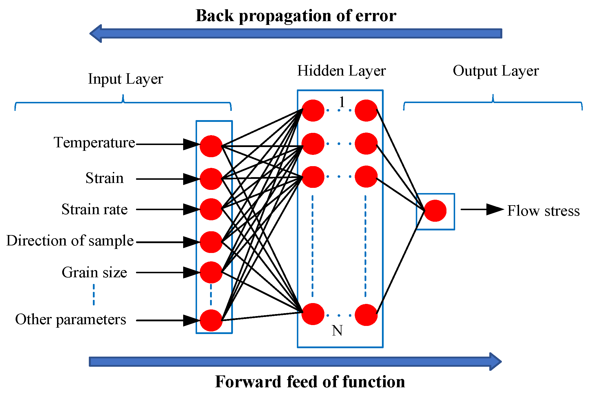
The BP (back-propagation) algorithm is one of the most commonly used feedforward neural network learning algorithms in materials modeling. The BP model has strong capacity for learning, generalization, fault tolerance, and nonlinear mapping. The typical structure of BP model is schematically illustrated in Figure 22, which consists of one input layer, one output layer, and one or more hidden layers [59,60,61,62,63].
In the BP model, the number of nodes in the input layer depends on the number of parameters affecting the actual deformation of the material, and the output layer parameter is the true stress of the material. The selection of the number of hidden layer neurons is a complex and important problem, which will have a great impact on the performance of the BP neural network. If the number of hidden layer neurons is too small, the BP network cannot converge during model training. On the contrary, if there are too many neurons in the hidden layer, the training data will be over-fitted, which will prolong the learning time of the network and reduce the generalization ability of the network. There is no rigid rule to find the number of neurons in the hidden layer, but it can be determined according to empirical Equation (96) [59] or Equation (97) [60]:
M = n + m + a
M = k 10 ( n + m )
where M is the number of hidden layer neurons, n is the number of neurons in the input layer, m is the number of neurons in the output layer, a is a positive integer ranging from 1 to 10, and k is the number of training set.
In addition to the number of hidden layer neurons, other structural parameters of BP neural network, such as the number of hidden layers, transfer function, and training function, will also have a great impact on the convergence speed and accuracy of the neural network model [61,62]. The Sigmoid function is usually used as the excitation function of hidden layer neurons, and the Purelin function as the excitation function of output layer neurons. The output Opj of the p training sample unit j from the input layer to the hidden layer can be expressed as
O p j = f ( N j ) = 1 1 + exp [ ( w i j X j + θ j ) ]
where Nj is the input of jth neuron in the hidden layer, wij is the connection weight between the input layer and the hidden layer, Xj is the output of jth neuron in the input layer to the hidden layer, and θj is the threshold of the input layer to the hidden layer.
Through modifying the connection weight among different layers and the threshold among different neurons, the high precision modeling with complex nonlinear characteristics can be completed. However, in order to realize the prediction of material flow stress, it is necessary to train the BP model with the help of experimental data.
Since the experimental data were measured in different units and value ranges, such as temperature, strain, strain rate, and stress, if the experimental data are directly used for model training, the convergence speed and accuracy of the model will decrease, or even not converge [63,64]. Therefore, the input and output of training samples and test samples based on experimental data must be normalized into dimensionless units before training. Through normalization processing, all input and output data are converted into numbers between 0 and 1, so as to eliminate the difference of orders of magnitude between experimental data of different dimensions.
In addition, the choice of the training function and parameters of the neural network model also has a great influence on the convergence speed and prediction accuracy. When the tansig and purelin functions are selected as network inter-layer transfer functions, the trainlm function of the Levenberg–Marquardt algorithm is used as a training function to optimize the BP algorithm; this will effectively reduce the number of iterations of the model and improve the convergence speed and accuracy [61,62,63].

4.2. Applications of (BP) Neural Network

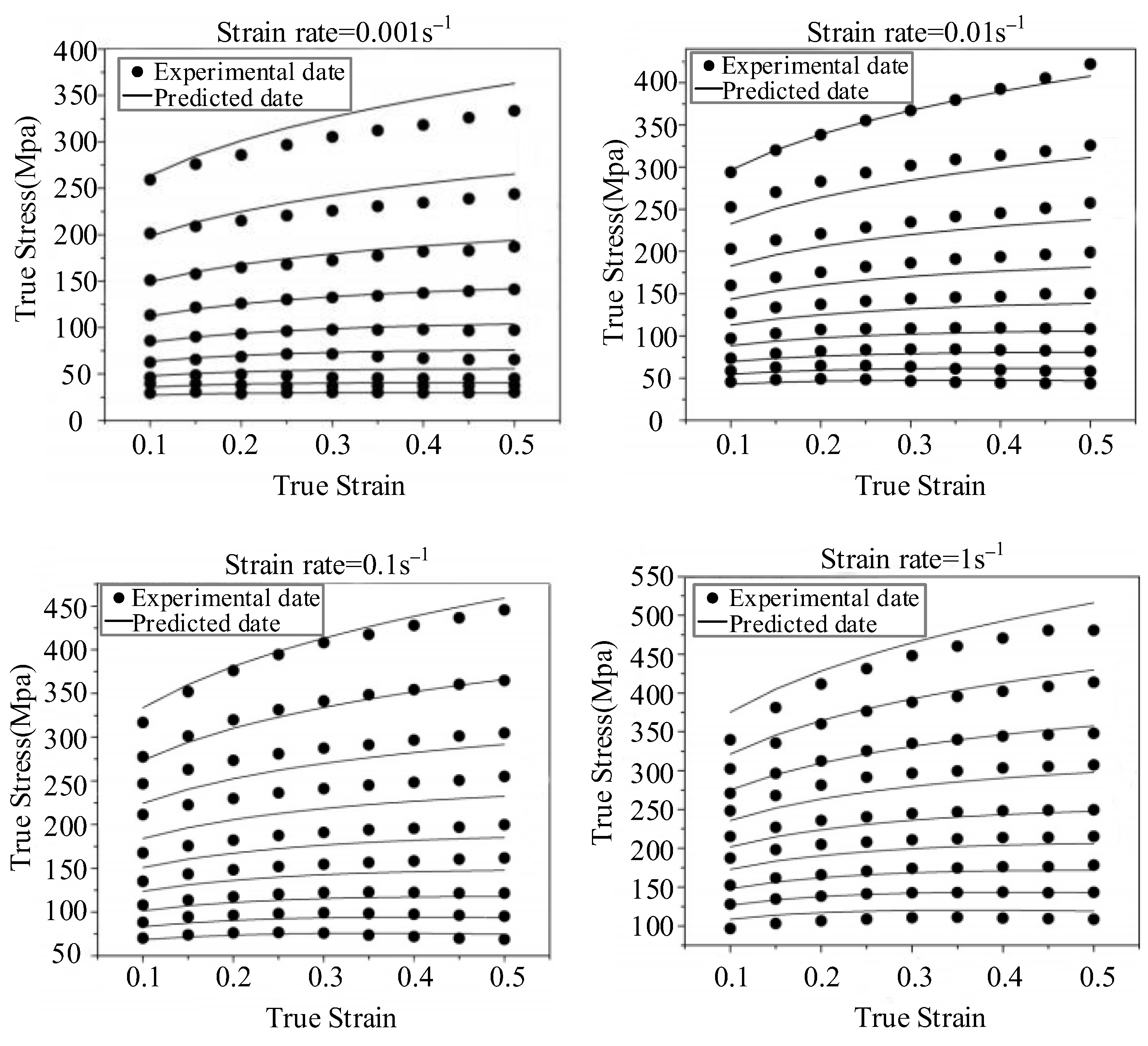
At present, the ANN model has been widely used to predict the microstructure evolution and mechanical properties of metal materials in plastic deformation. Sheikh et al. [65] used the artificial neural network model to predict the flow stress of aluminum alloy (AA5083), trained the neural network with the feedforward and back propagation algorithm, and calculated the stress–strain curves in different regions, which were compared with the experimental data to verify the reliability of the prediction, as shown in Figure 23.
Yan et al. [66] established the Arrhenius constitutive equation and artificial Neural network (ANN) model to study the flow behavior of Al-6.2Zn-0.70Mg-0.30Mn-0.17Zr aluminum alloy; the experimental and computational results are shown in Figure 24. The results show that the well-trained neural network model can describe the real stress–true strain curve well. Sabokpa et al. [67] have successfully predicted the mechanical properties of AZ81 magnesium alloy under different temperature conditions by using the BP algorithm, and pointed out that the BP network model can reflect the complex nonlinear relationship between the ultimate properties of alloys and the deformation temperature. In addition, Li et al. [68] and Haghdadi et al. [69] also compared the prediction ability of the traditional constitutive model and the BP model for different metal materials, and their research results showed that the prediction ability of the BP model was more accurate than that of the traditional constitutive model.
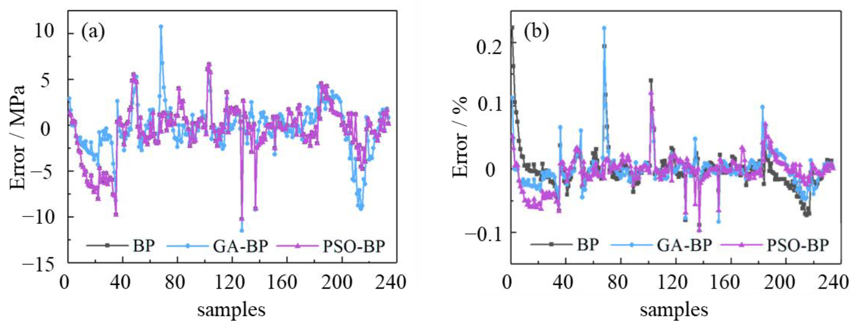
However, the BP neural network has some inherent flaws, such as the need to learn a large number of sample data to ensure the prediction accuracy, the slow learning speed, and tendency of falling into local minimum value and network instability [70,71,72,73]. Therefore, it is necessary to optimize the BP neural network to obtain a more accurate and reliable network model and better prediction performance. Ding et al. [74] used the genetic algorithm (GA) and particle swarm optimization (PSO) algorithm to optimize BP neural network, respectively. On this basis, the flow stress of 6061 aluminum alloy under different heat treatment conditions was predicted, as shown in Figure 25. Although the particle swarm optimization (PSO) algorithm is similar to the genetic algorithm, but the particle swarm optimization (PSO) algorithm has fewer parameters, simpler principles, and easier implementation. Gao et al. [75] used the BP model optimized by the genetic algorithm (GA) to predict the plastic deformation behavior of NiCoCrFe high-entropy alloy in the range of large strain rate (10−4–6000 s−1). The research results show that the GA-BP model has higher prediction accuracy. The optimized BP model can avoid the complex physical deformation mechanism of the material and easily predict the plastic deformation behavior of the metal under the complex deformation conditions such as high strain rate and high temperature.
The ANN model has high prediction accuracy of and can be easily optimized by a computer. The ANN model is especially suitable for dynamic response of material mechanical properties under complex deformation conditions. These characteristics determine that the artificial neural network model is suitable for finite element simulation of the material deformation process. In modern scientific research, the finite element numerical simulation plays an increasingly important role in many fields [76,77]. However, the accuracy of numerical simulation results is closely related to geometric boundaries such as material models.
In the numerical simulation model of aluminum alloy deformation behavior, Stoffel [77] used the ANN constitutive model instead of the traditional physical constitutive model to accurately predict the dynamic response of the aluminum alloy sheet sample under impact load. Bobbili [78] applied the ANN constitutive model to ABAQUS numerical simulation software and successfully predicted the dynamic impact deformation behavior of Ti-13NB-13Zr titanium alloy.
However, the prediction accuracy of the ANN model is greatly affected by the training database, so it is necessary to have a large enough test results database to train the model, which will lead to the increase of the test cost. Therefore, based on the limited test data, a numerical simulation method is developed which can quickly build a database for neural network model training. This will be an effective way to improve the prediction accuracy and application of a neural network model. For example, Gao [75] used the crystal plastic finite element model to build a training database, which is an effective means.
The ANN model has obvious advantages in finite element simulation. However, the ANN model cannot reflect the action mechanism of various internal influencing factors during plastic deformation of materials, and also cannot replace the physical constitutive model. Therefore, the physical constitutive model and ANN model will have their respective advantages in different application fields.

5. Conclusions

In this paper, the constitutive models of metal material are reviewed. According to their different mechanisms and characteristics, they can be divided into three types, namely the phenomenological model, microscopic model, and artificial neural network model. For each model, typical examples are given and their applicable conditions, advantages, and disadvantages are analyzed:
(1) The phenomenological model can be used to determine the constitutive relationship model of materials by means of regression analysis of experimental data. The solution process is relatively simple, but it cannot reflect the microscopic deformation mechanism of materials. Therefore, it is necessary to continuously modify to couple the effects of strain, strain rate, and temperature on the deformation behavior of materials.
(2) The microscopic constitutive model based on thermodynamics and dynamics theory can accurately characterize the microscopic deformation mechanism of materials under complex deformation conditions, and it also can accurately predict the flow stress of materials. However, compared with the macroscopic constitutive model, the microscopic constitutive model has more material parameters, which requires more complex experiments and processing methods. Therefore, the engineering application of the model is limited to a certain extent.
(3) As a new method, the artificial neural network (ANN) models are increasingly used to predict the flow stress of materials under complex deformation conditions, and it is suitable for finite element simulation of the material deformation process. However, the application of the ANN models largely depends on the training database, and cannot reflect the action mechanism of various internal influencing factors during plastic deformation of materials.

Author Contributions

X.J., methodology, investigation, review and editing, and supervision. K.H., original draft preparation and visualization. Z.L., visualization and review. Z.F., visualization and review. All authors have read and agreed to the published version of the manuscript.

Funding

The research is supported by the National Natural Science Foundation of China (52205384), the China Postdoctoral Science Foundation (2021M291604), the Jiangsu Postdoctoral Research Funding Program (2021K258B), the High-Level (Higher Education) Science Foundation of Nanjing Forestry University (GXL2018020), and the Youth Science and Technology Innovation Foundation of Nanjing Forestry University (CX2018027).

Conflicts of Interest

No conflict of interest exits in the submission of this manuscript, and the manuscript is approved by all authors for publication. The work submitted was original research, has not been published previously and is not under consideration for publication elsewhere in whole or in part. All the authors listed have approved the manuscript.

References

  1. Xiao, J.; Li, D.S.; Li, X.Q.; Deng, T.S. Constitutive modeling and microstructure change of Ti–6Al–4V during the hot tensile deformation. J. Alloys Compd. 2012, 541, 346–352. [Google Scholar] [CrossRef]
  2. Ashtiani, H.R.R.; Parsa, M.H.; Bisadi, H. Constitutive equations for elevated temperature flow behavior of commercial purity aluminum. Mater. Sci. Eng. A 2012, 545, 61–67. [Google Scholar] [CrossRef]
  3. Lin, Y.C.; Chen, M.S.; Zhong, J. Study of metadynamic recrystallization behaviors in a low alloy steel. J. Mater. Process. Technol. 2008, 209, 2477–2482. [Google Scholar] [CrossRef]
  4. Lin, Y.C.; Chen, M.S.; Zhong, J. Effects of deformation temperatures on stress/strain distribution and microstructural evolution of deformed 42CrMo steel. Mater. Des. 2008, 30, 908–913. [Google Scholar] [CrossRef]
  5. Lin, Y.C.; Chen, M.S.; Zhong, J. Constitutive modeling for elevated temperature flow behavior of 42CrMo steel. Comput. Mater. Sci. 2007, 42, 470–477. [Google Scholar] [CrossRef]
  6. Lin, Y.C.; Chen, M.S.; Zhong, J. Study of static recrystallization kinetics in a low alloy steel. Comput. Mater. Sci. 2008, 44, 316–321. [Google Scholar] [CrossRef]
  7. Lin, Y.C.; Chen, M.S. Study of microstructural evolution during static recrystallization in a low alloy steel. J. Mater. Sci. 2009, 44, 835–842. [Google Scholar] [CrossRef]
  8. Pu, B.; Song, P.; Li, W.B.; Yao, W.J.; Wang, X.M. Plastic deformation behavior and constitutive modeling of Cu-50Ta alloy during hot compression. Mater. Res. Express 2022, 9, 016517. [Google Scholar] [CrossRef]
  9. Shin, H.; Kim, J.B. A Phenomenological Constitutive Equation to Describe Various Flow Stress Behaviors of Materials in Wide Strain Rate and Temperature Regimes. J. Eng. Mater. Technol. 2010, 132, 021009. [Google Scholar] [CrossRef]
  10. Rusinek, A.; Rodriguez-Martinez, J.A.; Arias, A. A thermo-viscoplastic constitutive model for FCC metals with application to OFHC copper. Int. J. Mech. Sci. 2009, 52, 120–135. [Google Scholar] [CrossRef]
  11. Gao, Y.L.; Sun, X.M. On the parameters of dynamic deformation and damage models of aluminum alloy 6008-T4 used for high-speed railway vehicles. Explos. Shock. Waves 2021, 41, 118–129. [Google Scholar]
  12. Ru, Y.F.; Zhang, L.L.; Liu, W.; Chen, G.; Dou, W.Y. Inverse Determination Method of Johnson-Cook Model Parameters Based on the Stress State Test of Notched Specimens. J. Mech. Eng. 2021, 57, 60–70. [Google Scholar]
  13. Zhang, H.J.; Wen, W.D.; Cui, H.T. Behaviors of IC10 alloy over a wide range of strain rates and temperatures: Experiments and modeling. Mater. Sci. Eng. A 2008, 504, 99–103. [Google Scholar] [CrossRef]
  14. Lin, Y.C.; Chen, X.M. A combined Johnson–Cook and Zerilli–Armstrong model for hot compressed typical high-strength alloy steel. Comput. Mater. Sci. 2010, 49, 628–633. [Google Scholar] [CrossRef]
  15. Vural, M.; Caro, J. Experimental analysis and constitutive modeling for the newly developed 2139-T8 alloy. Mater. Sci. Eng. A 2009, 520, 56–65. [Google Scholar] [CrossRef]
  16. Khan, A.S.; Huang, S.J. Experimental and theoretical study of mechanical behavior of 1100 aluminum in the strain rate range 10-5-104s-1. Int. J. Plast. 1992, 8, 397–424. [Google Scholar] [CrossRef]
  17. Yu, H.D.; Guo, Y.J.; Zhang, K.Z. Constitutive model on the description of plastic behavior of DP600 steel at strain rate from 10−4 to 103s−1. Comput. Mater. Sci. 2009, 46, 36–41. [Google Scholar] [CrossRef]
  18. Khan, A.S.; Liang, R.Q. Behaviors of three BCC metal over a wide range of strain rates and temperatures: Experiments and modeling. International Journal of Plasticity, 1999, 1 A combined Johnson–Cook and Zerilli–Armstrong model for hot compressed typical high-strength alloy steel. Int. J. Plast. 1999, 5, 1089–1109. [Google Scholar] [CrossRef]
  19. Khan, A.S.; Suh, Y.S.; Kazmi, R. Quasi-static and dynamic loading responses and constitutive modeling of titanium alloys. Int. J. Plast. 2004, 20, 2233–2248. [Google Scholar] [CrossRef]
  20. Khan, A.S.; Suh, Y.S.; Chen, X.; Takacs, L.; Zhang, H. Nanocrystalline aluminum and iron: Mechanical behavior at quasi-static and high strain rates, and constitutive modeling. Int. J. Plast. 2006, 22, 195–209. [Google Scholar] [CrossRef]
  21. Farrokh, B.; Khan, A.S. Grain size, strain rate, and temperature dependence of flow stress in ultra-fine grained and nanocrystalline Cu and Al: Synthesis, experiment, and constitutive modeling. Int. J. Plast. 2008, 25, 715–732. [Google Scholar] [CrossRef]
  22. Fields, D.S.; Bachofen, W.A. Determination of strain hardening characteristics by torsion testing. ASTM Proc. Am. Soc. Test. Mater. 1957, 57, 1259–1272. [Google Scholar]
  23. Cheng, Y.Q.; Zhang, H.; Chen, Z.H. Flow stress equation of AZ31 magnesium alloy sheet during warm tensile deformation. J. Mater. Process. Technol. 2008, 208, 29–34. [Google Scholar] [CrossRef]
  24. Zhang, X.H. Experimental and Numerical Study of Magnesium Alloy during Hot Working Process. PhD Thesis, Shanghai Jiaotong University, Shanghai, China, 2003. [Google Scholar]
  25. Chen, Y.Y.; Li, M.Q.; Li, L. Kinetic variables based constitutive model for high temperature deformation of Ti-46.5Al–2Nb–2Cr. J. Mater. Res. Technol. 2021, 15, 3525–3537. [Google Scholar] [CrossRef]
  26. Yoo, J.D.; Kim, M.C.; Kim, E.J.; Razali, M.K.; Joun, M.S. Flow stress characterization of magnesium alloys at elevated temperatures: A review. J. Phys. Conf. Ser. 2021, 2047, 012002. [Google Scholar] [CrossRef]
  27. Spigarelli, S.; El Mehtedi, M. A New Constitutive Model for the Plastic Flow of Metals at Elevated Temperatures. J. Mater. Eng. Perform. 2014, 23, 658–665. [Google Scholar] [CrossRef]
  28. Brown, C.; McCarthy, T.; Chadha, K.; Rodrigues, S.; Aranas, C., Jr.; Saha, G.C. Constitutive modeling of the hot deformation behavior of CoCrFeMnNi high-entropy alloy. Mater. Sci. Eng. A 2021, 826, 141940. [Google Scholar] [CrossRef]
  29. Shi, H.; McLaren, A.J.; Sellars, C.M.; Shahani, R.; Bolingbroke, R. Constitutive equations for high temperature flow stress of aluminium alloys. Mater. Sci. Technol. 1997, 13, 210–216. [Google Scholar] [CrossRef]
  30. Guan, S.K.; Wu, L.H.; Wang, L.G. Flow stress and microstructure evolution of semi-continuous casting AZ70 Mg-alloy during hot compression deformation. Trans. Nonferrous Met. Soc. China 2008, 18, 315–320. [Google Scholar] [CrossRef]
  31. Chae, D.; Koss, D.A. Damage Accumulation and Failure of HY-100 Steel.Metallurgical and Materials Transactions, A. Phys. Metall. Mater. Sci. 2001, 32, 2985–2994. [Google Scholar]
  32. Lin, Y.C.; Chen, M.S.; Zhong, J. Effect of temperature and strain rate on the compressive deformation behavior of 42CrMo steel. J. Mater. Process. Technol. 2007, 205, 308–315. [Google Scholar] [CrossRef]
  33. Molinari, A.; Ravichandran, G. Constitutive modeling of high-strain-rate deformation in metals based on the evolution of an effective microstructural length. Mech. Mater. 2005, 37, 737–752. [Google Scholar] [CrossRef]
  34. Naderi, M.; Durrenberger, L.; Molinari, A.; Bleck, W. Constitutive relationships for 22MnB5 boron steel deformed isothermally at high temperatures. Mater. Sci. Eng. A 2007, 478, 130–139. [Google Scholar] [CrossRef]
  35. Durrenberger, L.; Molinari, A. Modeling of Temperature and Strain-Rate Effects in Metals Using an Internal Variable Model. Exp. Mech. 2009, 49, 247–255. [Google Scholar] [CrossRef]
  36. Durrenberger, L.; Molinari, A.; Rusinek, A. Internal variable modeling of the high strain-rate behavior of metals with applications to multiphase steels. Mater. Sci. Eng. A 2008, 478, 297–304. [Google Scholar] [CrossRef]
  37. Cerik, B.C.; Choung, J. Rate-dependent combined necking and fracture model for predicting ductile fracture with shell elements at high strain rates. Int. J. Impact Eng. 2020, 146, 103697. [Google Scholar] [CrossRef]
  38. He, X.; Liu, L.; Zeng, T.; Yao, Y. Micromechanical modelling of work hardening for coupling microstructure evolution, dynamic recovery and recrystallization: Application to high entropy alloys. Int. J. Mech. Sci. 2020, 177, 105567. [Google Scholar] [CrossRef]
  39. Zerilli, F.J.; Armstrong, R.W. Dislocation-mechanics-based constitutive relations for material dynamics calculations. J. Appl. Phys. 1987, 61, 1816–1825. [Google Scholar] [CrossRef] [Green Version]
  40. Zhang, H.; Wen, W.; Cui, H.; Xu, Y. A modified Zerilli–Armstrong model for alloy IC10 over a wide range of temperatures and strain rates. Mater. Sci. Eng. A 2009, 527, 328–333. [Google Scholar] [CrossRef]
  41. Samantaray, D.; Mandal, S.; Borah, U.; Bhaduri, A.K.; Sivaprasad, P.V. A thermo-viscoplastic constitutive model to predict elevated-temperature flow behaviour in a titanium-modified austenitic stainless steel. Mater. Sci. Eng. A 2009, 526, 1–6. [Google Scholar] [CrossRef]
  42. Preston, D.L.; Tonks, D.L.; Wallace, D.C. Model of plastic deformation for extreme loading conditions. J. Appl. Phys. 2002, 93, 211. [Google Scholar] [CrossRef] [Green Version]
  43. Kim, J.B.; Shin, H.H. Comparison of plasticity models for tantalum and a modification of the PTW model for wide ranges of strain, strain rate, and temperature. Int. J. Impact Eng. 2009, 36, 746–753. [Google Scholar] [CrossRef]
  44. Rusinek, A.; Klepaczko, J.R. Shear testing of a sheet steel at wide range of strain rates and a constitutive relation with strain-rate and temperature dependence of the flow stress. Int. J. Plast. 2001, 17, 87–115. [Google Scholar] [CrossRef]
  45. Rusinek, A.; Rodríguez-Martínez, J.A. Thermo-viscoplastic constitutive relation for aluminium alloys, modeling of negative strain rate sensitivity and viscous drag effects. Mater. Des. 2009, 30, 4377–4390. [Google Scholar] [CrossRef]
  46. Goetz, R.L.; Seetharaman, V. Modeling Dynamic Recrystallization Using Cellular Automata. Scr. Mater. 1998, 38, 405–413. [Google Scholar] [CrossRef]
  47. Jin, Z.Y.; Juan, L.; Cui, Z.S.; Wei, D.L. Identification of nucleation parameter for cellular automaton model of dynamic recrystallization. Trans. Nonferrous Met. Soc. China 2010, 20, 458–464. [Google Scholar] [CrossRef]
  48. Ren, Z.; Pu, Z.P.; Liu, D.R. Prediction of grain-size transition during solidification of hypoeutectic Al-Si alloys by an improved three-dimensional sharp-interface model. Comput. Mater. Sci. 2022, 203, 111131. [Google Scholar] [CrossRef]
  49. Zhao, Y.; Pu, Z.; Wang, L.; Liu, D.R. Modeling of Grain Refinement and Nucleation Behavior of Mg-4Y-0.5Zr (wt.%) Alloy via Cellular Automaton Model. Int. J. Met. 2021, 16, 945–961. [Google Scholar] [CrossRef]
  50. Song, Y.; Jiang, H.; Zhang, L.; He, J.; Zhao, J. Integrated model for describing the microstructure evolution of the inoculated Al-Zn-Mg-Cu alloys in continuous solidification. Results Phys. 2021, 26, 104465. [Google Scholar] [CrossRef]
  51. Gu, C.; Lu, Y.; Ridgeway, C.D.; Cinkilic, E.; Luo, A.A. Three-dimensional cellular automaton simulation of coupled hydrogen porosity and microstructure during solidification of ternary aluminum alloys. Sci. Rep. 2019, 9, 13099. [Google Scholar] [CrossRef] [Green Version]
  52. Steinberg, D.J.; Cochran, S.G.; Guinan, M.W. A constitutive model for metals applicable at high-strain rate. J. Appl. Phys. 1980, 51, 1498–1504. [Google Scholar] [CrossRef] [Green Version]
  53. Steinberg, D.J.; Lund, C.M. A constitutive model for strain rates from 10-4 to10-6S-1. J. Appl. Phys. 1989, 65, 1528. [Google Scholar] [CrossRef]
  54. Zaretsky, E.B.; Frage, N.; Ratzker, B.; Kalabukhov, S.; Mayseless, M. Impact response of a tungsten heavy alloy over 23–1100 °C temperature range. J. Appl. Phys. 2021, 129, 125902. [Google Scholar] [CrossRef]
  55. Brown, J.L.; Knudson, M.D.; Alexander, C.S.; Asay, J.R. Shockless compression and release behavior of beryllium to 110 GPa. J. Appl. Phys. 2014, 116, 411. [Google Scholar] [CrossRef]
  56. Li, W.; Kou, H.; Zhang, X.; Ma, J.; Li, Y.; Geng, P.; Wu, X.; Chen, L.; Fang, D. Temperature-dependent elastic modulus model for metallic bulk materials. Mech. Mater. 2019, 139, 103194. [Google Scholar] [CrossRef]
  57. Yang, X.; Zeng, X.; Wang, F.; Zhao, H.; Chen, J.; Wang, Y. A modified Steinberg-Cochran-Guinan model applicable to solid-liquid mixed zone along the principle Hugoniot. Mech. Mater. 2021, 155, 103775. [Google Scholar] [CrossRef]
  58. Mishra, S.K.; Brahma, A.; Dutta, K. Prediction of mechanical properties of Al-Si-Mg alloy using artificial neural network. Sādhanā 2021, 46, 139. [Google Scholar] [CrossRef]
  59. Singh, K.; Rajput, S.K.; Mehta, Y. Modeling of the hot deformation behavior of a high phosphorus steel using artificial neural network. Mater. Discov. 2017, 6, S2352924517300078. [Google Scholar] [CrossRef]
  60. Zhong, M.J.; Wang, K.L.; Lu, S.Q. Study on high temperature deformation behavior and BP neural network constitutive model of MoNb alloy. J. Plast. Eng. 2020, 27, 177–182. [Google Scholar]
  61. Jain, R.; Jain, A.; Rahul, M.R.; Kumar, A.; Dubey, M.; Sabat, R.K.; Samal, S.; Phanikumar, G. Development of ultrahigh strength novel Co–Cr–Fe–Ni–Zr quasi-peritectic high entropy alloy by an integrated approach using experiment and simulation. Materialia 2020, 14, 100896. [Google Scholar] [CrossRef]
  62. Lin, Q.Q.; Peng, D.S.; Zhu, Y.Z. Establishment of constitutive relationship model for 2519 aluminum alloy based on BP artificial neural network. J. Cent. South Univ. Technol. 2005, 12, 380–384. [Google Scholar] [CrossRef]
  63. Yu, Y.; Pan, Q.; Wang, W.; Huang, Z.; Xiang, S.; Lin, G.; Yan, J.; Liu, B. Microstructure Evolution and Constitutive Analysis of Al-Mg-Si-Ce-B Alloy during Hot Deformation. J. Mater. Eng. Perform. 2022, 31, 4707–4720. [Google Scholar] [CrossRef]
  64. Mi, X.; Tian, L.; Tang, A.; Kang, J.; Peng, P.; She, J.; Wang, H.; Chen, X.; Pan, F. A reverse design model for high-performance and low-cost magnesium alloys by machine learning. Comput. Mater. Sci. 2022, 201, 110881. [Google Scholar] [CrossRef]
  65. Sheikh, H.; Serajzadeh, S. Estimation of flow stress behavior of AA5083 using artificial neural networks with regard to dynamic strain ageing effect. J. Mater. Process. Technol. 2008, 196, 115–119. [Google Scholar] [CrossRef]
  66. Yan, J.; Pan, Q.L.; Li, A.D.; Song, W.B. Flow behavior of Al–6.2Zn–0.70Mg–0.30Mn–0.17Zr alloy during hot compressive deformation based on Arrhenius and ANN models. Trans. Nonferrous Met. Soc. China 2017, 27, 638–647. [Google Scholar] [CrossRef]
  67. Sabokpa, O.; Zarei-Hanzaki, A.; Abedi, H.R.; Haghdadi, N. Artificial neural network modeling to predict the high temperature flow behavior of an AZ81 magnesium alloy. Mater. Des. 2012, 39, 390–396. [Google Scholar] [CrossRef]
  68. Li, H.Y.; Wei, D.D.; Li, Y.H.; Wang, X.F. Application of artificial neural network and constitutive equations to describe the hot compressive behavior of 28CrMnMoV steel. Mater. Des. 2012, 35, 557–562. [Google Scholar] [CrossRef]
  69. Haghdadi, N.; Zarei-Hanzaki, A.; Khalesian, A.R.; Abedi, H.R. Artificial neural network modeling to predict the hot deformation behavior of an A356 aluminum alloy. Mater. Des. 2013, 49, 386–391. [Google Scholar] [CrossRef]
  70. Rao, K.P.; Prasad, Y.K.D.V. Neural network approach to flow stress evaluation in hot deformation. J. Mater. Process. Technol. 1995, 53, 552–566. [Google Scholar] [CrossRef]
  71. Wang, Y.J.; Wang, K.L.; Liu, S.Q. Hot Deformation Behavior and Forging Process Optimization of MoLa Alloy Based on Polar Reciprocity Model. Rare Met. Mater. Eng. 2018, 47, 2225–2231. [Google Scholar]
  72. Zhang, J.P.; Gao, P.F.; Fang, F. An ATPSO-BP neural network modeling and its application in mechanical property prediction. Comput. Mater. Sci. 2019, 163, 262–266. [Google Scholar] [CrossRef]
  73. Wan, P.; Wang, K.L.; Lu, S.Q. Constitutive modeling of Ti-2.7Cu alloy based on strain compensation and PSO-BP neural network. J. Eng. 2019, 47, 113–119. [Google Scholar]
  74. Ding, F.j.; Jia, X.D.; Hong, T.J.; Xu, Y.L. Flow Stress Prediction Model of 6061 Aluminum Alloy Sheet Based on GA-BP and PSO-BP Neural Networks. Rare Met. Mater. Eng. 2020, 49, 1840–1853. [Google Scholar]
  75. Gao, T.J.; Zhao, D.; Zhang, T.W.; Jin, T.; Ma, S.G.; Wang, Z.H. Strain-rate-sensitive mechanical response, twinning, and texture features of NiCoCrFe high-entropy alloy: Experiments, multi-level crystal plasticity and artificial neural networks modeling. J. Alloys Compd. 2020, 845, 155911. [Google Scholar] [CrossRef]
  76. Yuan, D.; Chen, J.; Yang, Y.; Zhang, L.; Liu, S.; Jiang, H.; Qian, N. Thermal Performance of the Thin Heat Pipe for Cooling of Solid-State Drives. Metals 2022, 12, 1786. [Google Scholar] [CrossRef]
  77. Stoffel, M.; Bamer, F.; Markert, B. Neural network based constitutive modeling of nonlinear viscoplastic structural response. Mech. Res. Commun. 2019, 95, 85–88. [Google Scholar] [CrossRef]
  78. Bonnili, R.; Madhu, V. Constitutive modeling and fracture behavior of a biomedical Ti-13Nb-13Zr alloy. Mater. Sci. Eng. A 2017, 700, 82–91. [Google Scholar]
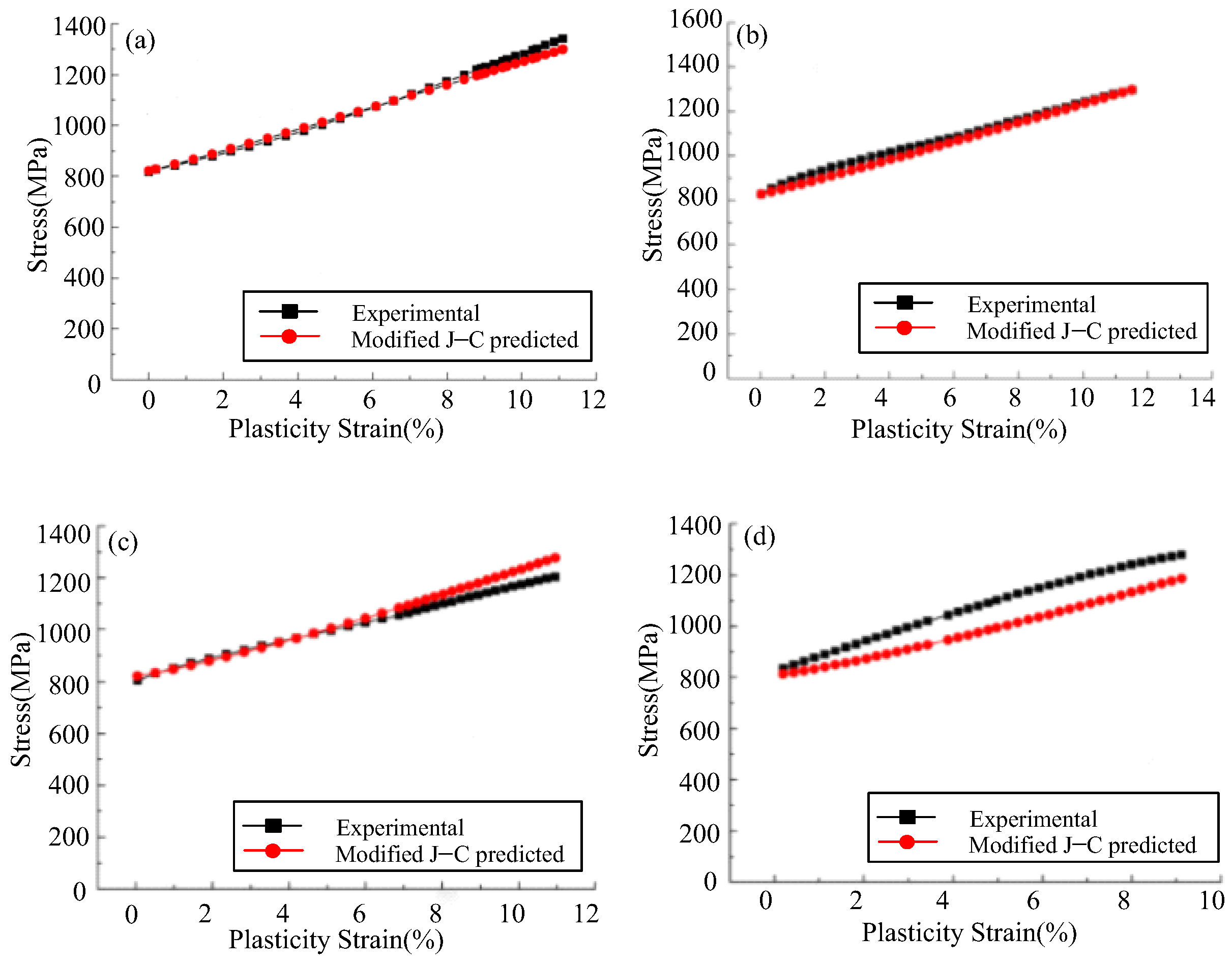
Figure 1. The predicted results of IC10 alloy based on the modified J–C model [13], (a) T = 25 °C, ε ˙ = 0.00001 s 1 , (b) T = 600 °C, ε ˙ = 0.0001 s 1 , (c) T = 700 °C, ε ˙ = 0.0001 s 1 , (d) T = 800 °C, ε ˙ = 0.0001 s 1 .
Metals 12 02077 g001
Figure 2. Flow stress comparison curves of 42CrMo, (a) 1223 K; (b) 1423 K [14].
Metals 12 02077 g002
Figure 3. Vural and Caro modified J–C model [15], (a) temperature dependence of flow stress at 10−4 s−1 reference strain rate; (b) effects of strain rate and temperature under dynamic loading.
Metals 12 02077 g003
Figure 4. Comparison of KH model predictions and experimental data at different strain rates [17].
Metals 12 02077 g004
Figure 5. The relation curve between   f ^ 2 ( ε ˙ p )   and   ln ε ˙ p / ε ˙ 0 p [17].
Metals 12 02077 g005
Figure 6. Comparison of the new constitutive model prediction data and experimental data [17].
Metals 12 02077 g006
Figure 7. The modified KHL model compared with J–C model [19].
Metals 12 02077 g007
Figure 8. Prediction results of mechanical properties of nanocrystalline aluminum based on the KHL model [20].
Metals 12 02077 g008
Figure 9. Prediction results of the KLF model under different mean particle sizes [21], (a) Cu; (b) Al.
Metals 12 02077 g009
Figure 10. Prediction results of the KLF model under different strain rates [21], (a) Cu (d = 32 nm); (b) Al (d = 82 nm).
Metals 12 02077 g010
Figure 11. Flow stress curve of AZ31 magnesium alloy [23].
Metals 12 02077 g011
Figure 12. The stress prediction results of AZ31 magnesium alloy based on the modified FB model [23].
Metals 12 02077 g012
Figure 13. The rheological properties of CoCrFeMnNi alloy [28], (a) 0.01 s−1; (b) 1 s−1.
Metals 12 02077 g013
Figure 14. The prediction results based on the DMR model [36], (a) TRIP800; (b) DP600; (c) TRIP700; (d) Fe-Mn.
Metals 12 02077 g014
Figure 15. Stage division of typical stress–strain relationship in HEAs [38].
Metals 12 02077 g015
Figure 16. The prediction results of IC10 alloy based on the modified ZA model [40]. (a) T = 293 K, ε ˙ = 0.001   s 1 , (b) T = 293 K, ε ˙ = 0.0001   s 1 , (c) T = 873 K°C, ε ˙ = 0.001   s 1 , (d) T = 973 K, ε ˙ = 0.0001   s 1 .
Metals 12 02077 g016
Figure 17. The predicted flow stresses of D9 alloy based on the Samantaray modified model [41].
Metals 12 02077 g017
Figure 18. The predicted flow stresses of tantalum based on the modified PTW model [43]. (a) T=473 K, ε ˙ = 2800   s 1 , T = 873 K, ε ˙ = 2200   s 1 , (b) T = 1073 K, ε ˙ = 29,001   s 1 .
Metals 12 02077 g018
Figure 19. NSRS description using extended RK model [45], (a) 0.00041 s−1; (b) 122 s−1.
Metals 12 02077 g019
Figure 20. Temperature sensitivity description using the extended RK model [45].
Metals 12 02077 g020
Figure 21. Comparison of simulated strain curves of OFHC copper [47].
Metals 12 02077 g021
Figure 22. Schematic diagram of the BP neural network model.
Metals 12 02077 g022
Figure 23. Comparison of prediction results between experimental data and non-sampling results [65].
Metals 12 02077 g023
Figure 24. The predicted results of aluminum alloy based on ANN molde [66], (a) 0.01 s−1; (b) 0.1 s−1; (c) 1 s−1; (d) 10 s−1.
Metals 12 02077 g024
Figure 25. The prediction error and error ratio of neural network model (the data from [74]), (a) prediction error; (b) prediction error ratio.
Metals 12 02077 g025
Table 1. The characteristics of the phenomenological constitutive model.
Model NameCharacteristics and Application Conditions
Johnson–Cook (J–C) Model
  • The model has few parameters and is easy to solve
  • The influence of deformation temperature and strain rate is taken into account
  • Easy model correction, modified J–C model
Khan–Huang (KH) Model
  • It consists of elastic component and plastic component
  • Applicable to a wide range of strain rates (10−5–104 s−1)
  • Temperature effects are not taken into account
Khan–Huang–Liang (KHL) Model
  • The modified model of the KH model
  • Consider the temperature effect of deformation
Khan–Liang–Farrokh (KLF) Model
  • The modified model of the KHL model
  • Both temperature effect and strain rate effect are taken into account
  • The grain size effect of the material is considered
Fields–Backofen (FB) Model
  • Both temperature effect and strain rate effect are taken into account
  • The model has few parameters
  • The parameter fitting process is simple
Hansel–Spittel Model
  • Combined the classical strain rate power-law model with the Hollomon and Swift model
  • The effects of both temperature and strain rate are considered
  • The model can be solved by regression analysis
Arrhenius Model
  • The influence of strain rate and temperature at high temperature is considered
  • It can predict the peak stress of the material
  • The modification of model parameters can be suitable for large deformation
Molinari–Ravichandran Model
  • The effects of temperature, strain rate, and grain size are considered comprehensively
  • Based on the microscopic characteristics of the material
  • The DMR model can characterize the thermal and viscoplastic behavior
Table 2. The characteristics of microscopic constitutive model.
Model NameCharacteristics and Application Conditions
Zerilli–Armstrong Molde
(ZA Model)
  • Based on the dislocation dynamics theory
  • The influence of deformation temperature, strain rate, and the average size of grains are taken into account
  • The influence of crystal structure is distinguished
  • It can be used to characterize the plastic deformation behavior of the thermal activated region
Preston–Tonks–Wallace (PTW) Model
  • The effect of strain rate mechanism is considered, dislocation slip region, transition region, and ultra-high strain rate region
  • Applicable to a wide range of strain rates
  • It can characterize the nonlinear dislocation effect under impact load
Rusinek–Klepaczko Model
(RK Model)
  • The flow stress is decomposed into internal stress and effective stress
  • The influence of temperature on Young’s modulus is considered
  • The temperature effect and strain hardening are considered simultaneously
  • The modified RK model can describe the viscoplastic behavior of FCC material
Cellular Automaton Model
(CA Model)
  • Based on physical metallurgical principles
  • It can describe the microstructure evolution during dynamic recrystallization
  • The effects of temperature and strain rate on dynamic recrystallization are considered
Steinberg-Guinan Model
(SG Model)
  • The effects of temperature and pressure are considered
  • The effect of strain rate is not considered
  • It is suitable for high strain rate (>105 s−1) and high-pressure conditions
Steinberg-Lund Model
(SL Model)
  • The effects of temperature and pressure are considered
  • The flow stress is the sum of the thermal and non-thermal stress components
  • It can be used over a relatively wide range of strain rates (10−4–106 s−1)
Publisher’s Note: MDPI stays neutral with regard to jurisdictional claims in published maps and institutional affiliations.