Simulation and Microstructure Prediction of Resistance Spot Welding of Stainless Steel to Carbon Steel

Abstract

Joining of stainless steel to carbon steel is widely used in various industries. Resistance spot welding (RSW) is a suitable process for joining steel sheets. Due to the complexity and importance of optimizing the parameters, numerical simulation of this process was considered. In this research, the electrical-thermal-mechanical simulation of RSW of 304 stainless steel to St37 carbon steel was performed using finite element method (FEM). Then, the simulated weld nugget size was compared with the experimental results of optical microscopy (OM). In addition, diffusion of metallic elements of the steels in the molten region was simulated using Fick’s equation and compared with experimental results of energy-dispersive X-ray spectroscopy (EDS). It was shown that diffusion of Cr and Ni through the weld nugget, would make a new stainless steel structure. Microstructure prediction of the heat affected zone (HAZ) was performed using Koistinen–Marburger and Leblond–Devaux equations to predict the percentage of martensite and ferrite-perlite phases during the heating and cooling stages of the specimens from room temperature to the peak temperature and cooling down under the M_f temperature. The results of this simulation were validated by scanning electron microscopy (SEM) images and shear tensile and micro-hardness test results. The simulation results showed that increasing the heat input from 1250 A during 0.5 s to 3750 A during 1.5 s, increases the percentage of martensite, from 40% to 80%, in the HAZ and widens the martensite region.

1. Introduction

Joining of carbon steel and stainless steel has a wide range of applications, including in power generators, oil and gas industries, petrochemical industries, heat exchangers and boilers. Therefore, the dissimilar joining between these two steels is in focus [1].

Resistance spot welding (RSW) is one of the processes of joining sheet metals having high production rate and is widely used for connecting all types of steels. RSW is a kind of fusion welding process, where high currents, 1 to 5 kA, are passed through the workpiece and melting occurs at the interface of the sheets to be welded [2].

In RSW, there is a complex interaction of the thermal, electrical, and mechanical phenomena during the process. Moreover, physical and metallurgical properties of the materials to be welded undergo changes. The most important welding parameters include welding current, electrode force, welding time, holding time, and the electrode geometry. These parameters must be adjusted and optimized such that a weld nugget is formed [3]. Optimization of RSW process parameters, previously, used to be carried out experimentally in the laboratory. Although this method is very accurate and reliable, but it also has its disadvantages, the most important of which is the low speed of the testing process.

Nowadays, in many fields of research, numerical modeling has been used partly or fully as a proper replacement for experimental testing. There are several methods for modeling and optimization of RSW process. These methods include simple regression [4], response surface methodology [5], artificial neural networks [6], and also finite element method simulations (FEM).

Since the RSW method has complexity in the process and parameters, multi-physics methods should be used in simulating this process. FEM is a proper tool for simulating multi-physic models such as RSW process. In fact, a key challenge in RSW simulations is to consider the coupling between physics and the interaction between them. These physics include thermal, electrical, mechanical simulation, and microstructure prediction.

For the first time, the RSW process was simulated using the FEM method, considering the thermal-mechanical coupling by Nied et al. [7]. Browne and Chandler [8,9] performed this process by considering successive electrical-thermal and mechanical couplings. Considering factors such as mass transfer, momentum and magnetic field in the RSW process simulation was done by Wei and Ho [10]. Gupta and De [11], Feng et al. [12] and Khan and Xu [13] used the thermal-electrical-mechanical model to simulate this process. In Khan’s model, the effect of contact between parts including plates and electrodes were considered. Weld nugget size simulation in RSW process was performed by Anderson et al. [14], Eisazadeh et al. [15], Moshayedi et al. [16], and Eshraghi et al. [17], using FEM method and compared and validated with experimental results. In these research, it was observed that increasing the heat input, by increasing the current and welding time, increases the size of the nugget. Moshayedi et al. [16] showed that the size of the nugget increases with the increase of input heat. But after a certain size, the growth rate decreases with the increase of input heat, which reduces the production rate despite creating a solid structure.

Simulation of RSW for dissimilar welding of metals is of great importance due to the differences in physical and mechanical properties of the two metals, mixing of molten materials in the nugget and occurrence of other metallurgical phenomena. However, it has received less attention in research. In a study, Wang et al. [18] simulated the electrical-thermal and mechanical coupling of steel and aluminum joints. They also performed microstructure predictions of this process using temperature history and the kinetic equations for the formation of intermetallic compounds (IMCs). They showed that due to the indissolubility of the elements in the nugget region of these two dissimilar metals, two separate nuggets are actually formed, one on the aluminum side and the other on the steel side. Using FEM method, Dancette et al. [19] simulated the dissimilar welding of Usibor1500/DP600 high strength steel. Their model was created with the aim of predicting deformation and failure in this process. With the investigations carried out in previous studies, it was observed that the simulation of metallurgical phenomena in the RSW process, along with other physics, has received less attention from researchers.

Joining of stainless steel to carbon steel by RSW method has been considered in some studies. Marashi et al. [20] investigated the microstructure and failure behavior of dissimilar joining of austenitic stainless steel to galvanized carbon steel by RSW method. They observed a microstructure gradient in the HAZ through the base metal from martensite to pearlitic structure and the hardness changes from the nugget edge to the base metal. They also investigated the relationship between fracture mode and weld zone properties including size and microstructure. Charde et al. [21] characterized the dissimilar welding of 304 stainless steel to plain carbon steel. Ishak et al. [22] also studied the mechanical properties and impact resistance of 301 stainless steel and 1020 carbon steel. They studied and optimized the process parameters using response surface methodology (RSM) and Taguchi method. Sani et al. [23] simulated the vibration behavior of 304 stainless steel and 1010 carbon steel plates welded by RSW using FEM method.

By looking at the previous research, it can be seen that the joining of stainless steel to carbon steel using RSW has not been studied from the point of view of simulation. Therefore, considering the importance of the subject, in this research, this joint is investigated from an experimental and numerical perspective. In this research, electrical-thermal-mechanical and metallurgical simulations of RSW between 304 stainless steel and Carbon steel were performed using FEM method. The results, including the effect of current and time parameters on the weld nugget size, were validated with the experimental results. The distribution and exchange of elements between the two alloys in the nugget region were simulated using the Fick’s equation. The main innovation of the article compared to similar research is that in this research the prediction of the microstructure in the HAZ as well as the distribution of alloy elements in the melting zone of two dissimilar metals is considered. The results were validated with energy-dispersive X-ray spectroscopy (EDS) plots. Using the numerical results extracted from FEM simulation, microstructure predictions were performed by predicting microstructural changes in the heat affected zone (HAZ) of carbon steel. The Koistinen–Marburger equation was used to predict the percentage of martensite phase and the Leblond–Devaux equation was used to predict the percentage of ferrite and perlite. The results were validated by scanning electron microscopy (SEM) images of both HAZ and fractured sections, micro-hardness and shear tensile strength at different welding parameters.

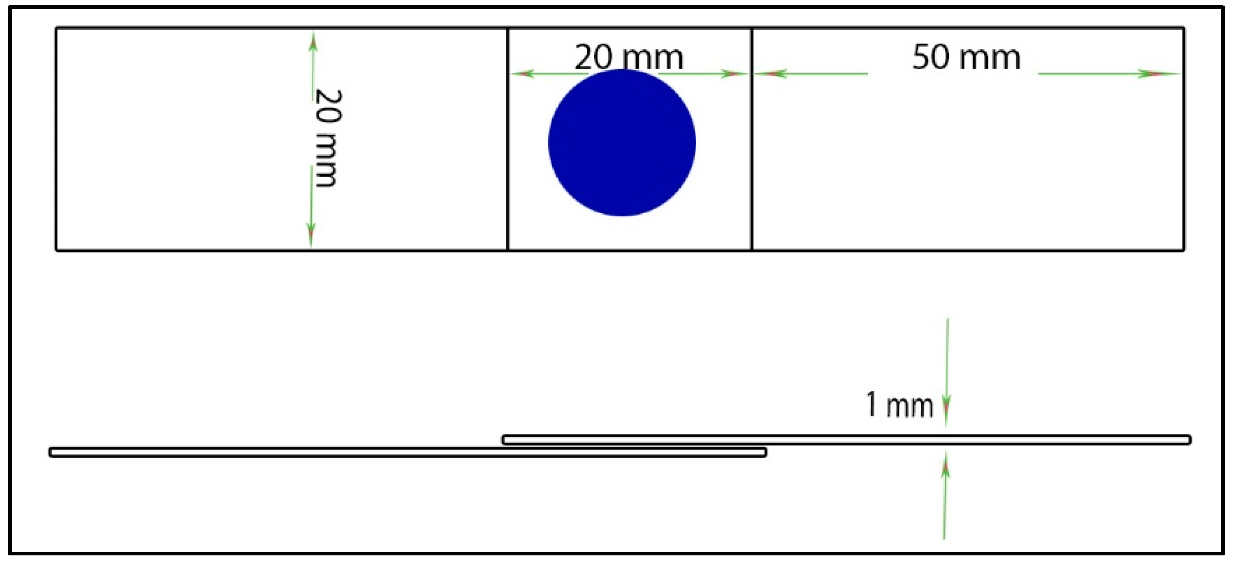
2. Materials and Methods

In this study, stainless steel plate (AISI304) and a St37 carbon steel sheet with a thickness of 1 mm were used. The chemical composition of these steels is given in

Table 1. Chemical composition of AISI304 and St37 steel.

Elements	C%	Si%	Mn%	Cr%	Ni%	P%	S%	Fe%
AISI304	0.03	0.35	2	18.02	8	0.01	0.003	balanced
St37	0.17	0.55	1.2	-	-	0.01	0.02	balanced

. These plates were degreased with acetone, after an initial polishing.

Dissimilar RSW was performed on stainless steel to carbon steel samples. The dimension of the samples were 30 $\times$ 30 $\times$ 1 mm (length * width * thickness). The copper electrode head that was connected to the parts was an imperfect cone with a lower diameter of 10 mm and an upper diameter of 20 mm. The voltage of the RSW machine was about 350 volts. After degreasing with acetone, the samples were welded at different currents and times according to

Table 2. Taguchi L9 design for current and time parameters.

I(A)	1250	2500	3750	1250	2500	3750	1250	2500	3750
t(S)	0.5	0.5	0.5	1	1	1	1.5	1.5	1.5

This experiment was designed according to L9 Taguchi orthogonal arrays.

Microstructure and Mechanical Analysis

In this study, the optical microscopy (OM) was used to evaluate the macrostructure of the samples. The samples were mounted by cold mounting, sanded to 2400 grit, polished and etched with Nital solution for microstructure analysis. To evaluate the weld zone and the heat affected zone (HAZ) of the steels, the samples were etched in Marble’s reagent solution containing HCl, H2O, and Cu2SO4, and examined by scanning electron microscopy (SEM). Moreover, the samples were examined by energy-dispersive X-ray spectroscopy (EDS) analysis from the perspective of element distribution in the fusion zone.

In order to determine the mechanical properties of joint, the micro-hardness and tensile shear test were performed. The tensile shear test was performed according to AWS/D8.9-97 standard, with a strain rate of 2 mm/min. The schematic image of the sample is shown according to Figure 1.

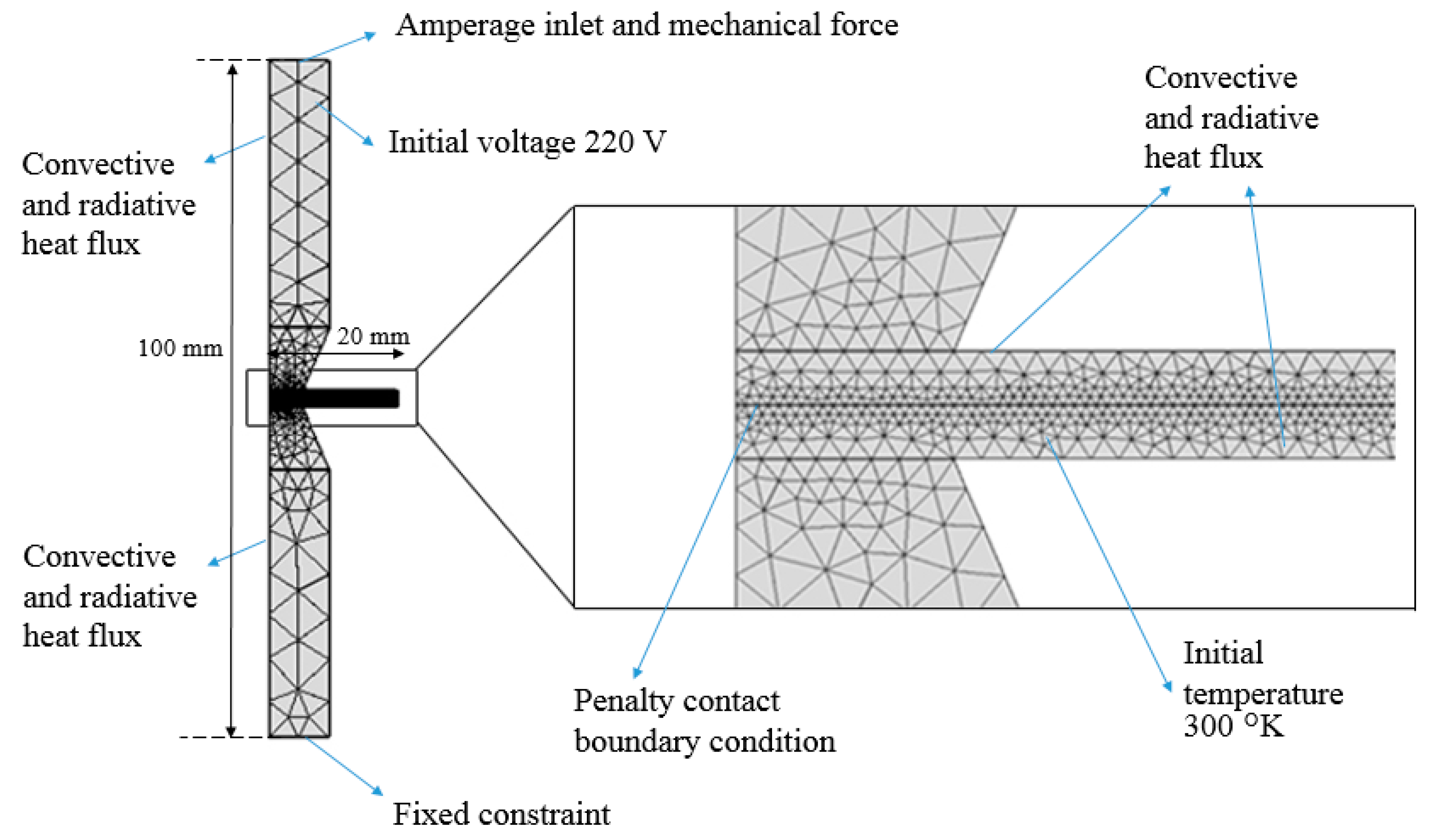
3. Model description

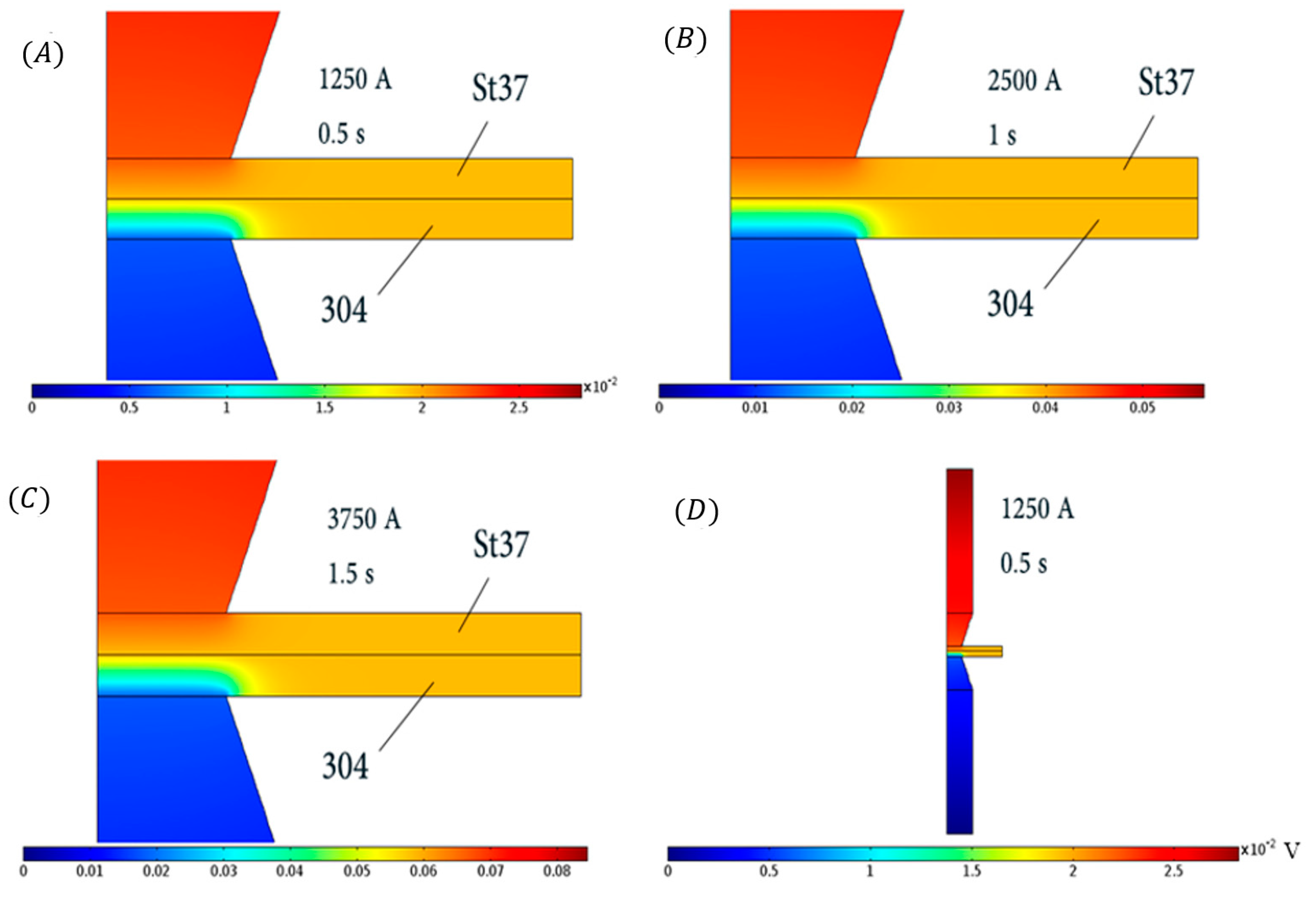
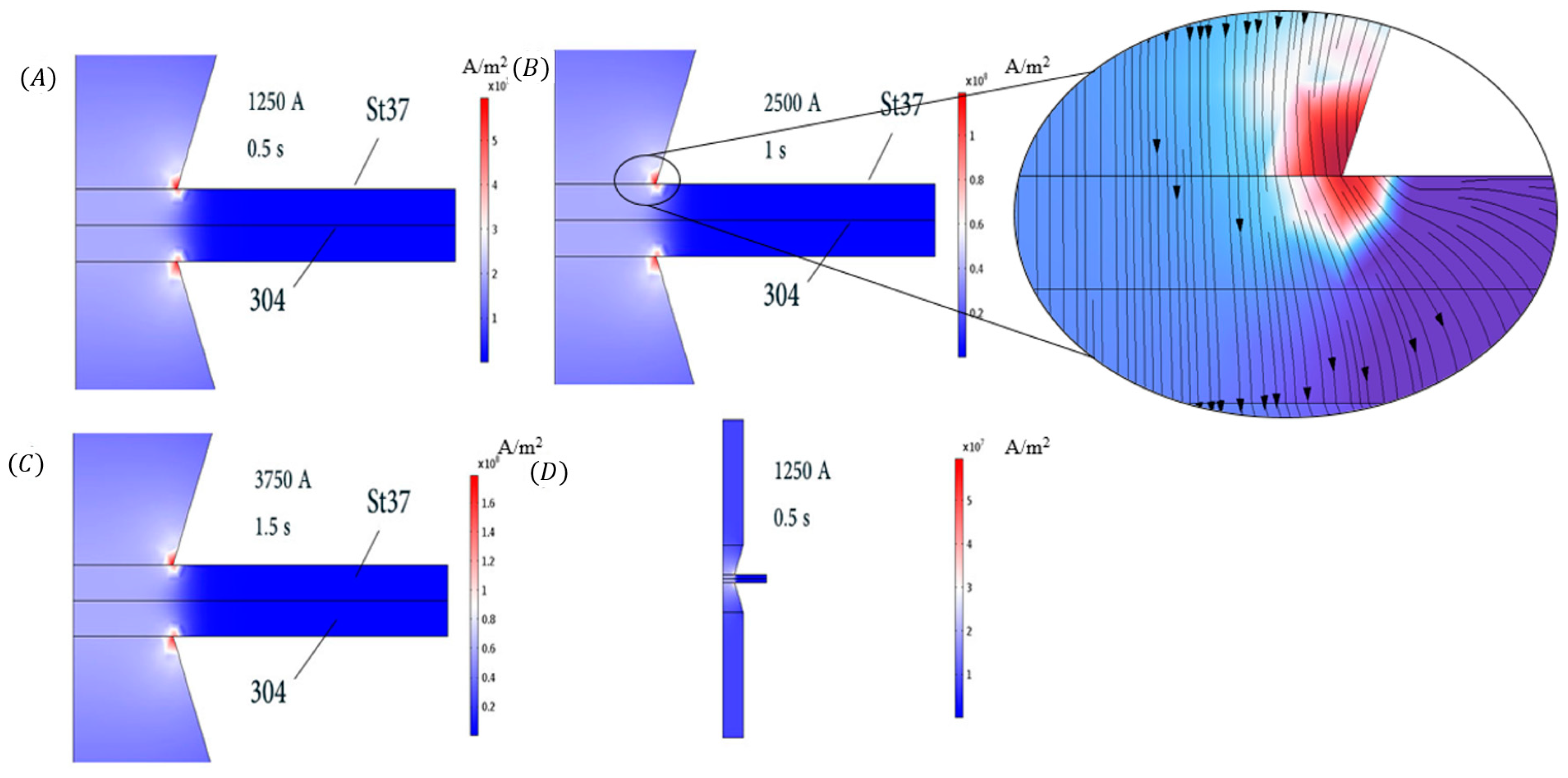
3.1. Electrical- Thermal and Mechanical Simulation

In order to predict the potential distribution and electric current along the parts, the Laplace equation according to Equation (1) was used:

$${\nabla }^2\varnothing =0$$

(1)

where $\varnothing$ is the electric field. It should be noted that the upper surface of the electrode was considered as the input terminal of the electric current. The pressure applied during the welding process creates an electrical connection between the parts. In this research, the pressure applied from the device to the welding electrodes is constant and equal to 2 kN. In this model, due to considering the penalty contact between the parts, applying pressure causes the nodes to contact and as a result, create an electric current between the nodes at the connection boundary.

According to the Fourier equation, the generated heat caused by the passage of electric current through the parts distributes through the samples according to Equation (2). This equation is considered for a transient (time dependent) solution:

$$\rho C_p\dot{T}=\nabla \left(k\nabla T\right)+\dot{Q}$$

(2)

where k is the heat transfer coefficient, ρ is density (Kg/m³), and C_p is the heat capacity coefficient (J/Kg.K). In addition, $\dot{Q}$ (W/m².s), according to Equation (3), is the heat generated by electrical current at the interface of the components:

$$\dot{Q}=R{I}^2$$

(3)

where R is the electrical resistivity and I is the current obtained in electrical simulation. The application of 220 V voltage was considered as the initial condition. Electric flux was applied from the upper surface of the electrode. Stainless steel, carbon steel, and copper temperature dependent material properties are extracted from previous research including Nandan et al.’s [24,25] and Moshayedi and Sattari-Far’s [16] works.

In this research, the initial temperature of the parts is assumed 300 (°K). Since the surface of the welding parts is in contact with air, the convection boundary condition was used in this model, which is obtained from Equation (4). In this equation, T is the ambient temperature equal to 300 (°K) and h (W/m².K) is the convection coefficient. Convection coefficient according to references for stainless steel is calculated according to Equation (5). The thermal radiation boundary condition was used according to Equation (6). This includes the radiation coefficient, ε, and the Stephen–Boltzmann coefficient, B. The radiation coefficient for steels is equal to 0.17 and the Stephen–Boltzmann coefficient is 5.67 × 10⁻⁸ (W/m².K⁴).

$$k\frac{\partial T}{\partial n}=h\left(T-T_a\right)$$

(4)

$$\mathrm{h}=0.0668\mathrm{T}\hspace{1em}\mathrm{T}<500 °\mathrm{C}$$

(5)

$$k\frac{\partial T}{\partial n}=B\epsilon \left(T^4-{T_0}^4\right)$$

(6)

Determination of transient strain distribution coupled with thermal-electrical physics is an important factor in simulating the weld interface and plates-electrodes interface. In this study, solid mechanics physics considering the elastic behavior of the materials and penalty contact condition between the interfaces were applied.

3.2. Solute Diffusion Simulation

In order to simulate Cr and Ni solutes distribution and diffusion in the molten weld zone, Fick’s second law, according to Equation (7) was applied. Since the diffusion of the solutes in the molten zone coincides with being in an electric field, the flux equation of Fick’s second law was modified with the Nernst–Einstein equation [26], according to Equation (8).

$$\rho \frac{\partial C_i}{\partial t}+\nabla J=0$$

(7)

$$J=-\left(\rho D_i+\rho C_{i}Z\frac{D_i}{RT}F\nabla V\right)$$

(8)

In the above equations, $C_i$ is the solute concentration, J is the diffusion flux, $D_i$ is the solute diffusion coefficient in molten iron, which is extracted from Ono and Matsumoto’s research [27] for Cr and Ni, Z is the charge number of elements, F is the Faraday’s constant, and V is the applied voltage. It should be noted that the simulation domain was the molten area which was obtained from the thermal simulation.

3.3. Microstructure Prediction

In this model, as the HAZ is exposed to heat due to RSW, phase changes in the HAZ is expected. In this study, the Leblond–Devaux (L-D) model, according to Equation (9) [28], was used to simulate the transformation of perlite to austenite, and conversely, in St37 steel. This model considers carbon-based phase transformations in the heat treatment processes of steels. In addition, Koistinen–Marburger (K-M) equation, according to Equation (10) [29] was used to investigate the formation of martensite in the HAZ.

$$\dot{X^d}=K_{s\to d}{X}^s-L_{s\to d}{X}^d$$

(9)

$$X^d=X_0{}^s\left(1-\exp \left(-\beta \left(M_s-T\right)\right)\right)$$

(10)

where $X^d$ is the destination fraction and $X^s$ is the source fraction, $K_{s\to d}$ and $L_{s\to d}$ are L-D constants extracted from Leblond et al.’s work [30], $\beta$ is the K-M constant and Ms is the martensitic transformation starting temperature.

In this research, a two-dimensional axisymmetric model was used. According to Figure 2, two copper electrodes and two steel sheets, with specific dimensions, were considered and the axis of symmetry was the midline. In this figure, additionally, the thermal, electrical, and mechanical boundary and initial conditions and geometrical dimensions are demonstrated. Triangular elements were used for meshing. In the boundary of the samples, the penalty contact boundary condition was used for more accuracy. An implicit solver was applied to solve the equations. All the geometry and physics were created and solved using COMSOL multiphysics software (version 6.1, COMSOLAB, Stockholm, Sweden).

4. Result and Discussion

As shown in Figure 3, the electric potential distribution is obtained by solving the Laplace equation. According to this simulation, it is observed that by increasing current, the average amount of electrical potential increases. This is while the input potential is the same. The reason for this is the dependence of the potential on the current and the resistivity, and also the resistivity of the parts are constant. Another issue is the constant potential at the electrodes. This is due to the low electrical resistivity of copper and its high electrical conductivity. Figure 4 demonstrates the electrical current distribution in the parts during RSW process. It can be seen that in all three input amperages, the general form of the current distribution is completely the same and only the magnitude of the values, as seen in the color bar, is different. It is observed that the average current is equal to the input current in the terminal. However, it is important to note that changing the welding geometry from the electrode input to the steel sheets results in a sharp increase in current. In addition, it can be noticed that a strong electric current concentration occurs in the parts, around the corners of the electrodes. By looking at the zoomed image, it can be seen that the current density is higher in the corner of the electrode and the density of current lines is also higher. It can also be seen that the direction of the current lines is from the electrode to the work piece. The reason for this is the existence of sharp points for entering and exiting the flow in these areas.

After simulating the electric current distribution (Figure 4), it is facilitated to evaluate the amount of heat generated at the interface boundary. Therefore, with the equations mentioned earlier, the temperature distribution in the welding zone at different currents and times is obtained as shown in Figure 5. As it can be noticed, the heat produced at the interface of the parts leads to the creation of a button-shaped fusion area. This region, at the points where the temperature is higher than the melting temperature, is the welding nugget. It can be seen from Figure 5A to c that increasing the current leads to an overall increase in temperature as well as an expansion of the welding area and HAZ. On the other hand, it can be seen that the heat does not reach the farthest areas of the sheet due to less time for heat diffusion and also the effect of intense heat transfer properties of copper, which attracts some of the generated heat. It should be noted that the maximum temperatures measured by thermocouples 2 mm near the weld nugget on the top surface of the specimen, were for 1250 A—0.5 s: 1120 degC, 2500 A—1 s: 1190 degC, and 3750 A—1.5 s: 1280 degC, which can be validated with the simulation results. The heating and cooling temperature history of the parts, extracted from the simulation results, according to Figure 5E, at three different points of the sample, 1250 A and 0.5 s, shows that in the central point of the welding zone of the part, a high temperature has been reached and then it is rapidly cooled, this phenomenon can be seen at point number 2, which is the edge of the welding nugget, with a lower temperature. It can be seen that the cooling slope of both points is almost similar to each other, which is because the surrounding points are colder and as a result, these points suddenly cool down. On the other hand, in point 3, which is in the HAZ region but has a greater distance from the nugget, it can be seen that the temperature reached less than 800 degC and then cooled down with a lower slope. The reason for this is the passage of less electric flux at this point and, as a result, lower temperature. In addition, due to the lower temperature compared to points 1 and 2, it has a lower cooling slope.

In RSW, the diameter of the weld nugget, the solidified joining interlayer between sheets, is the main measure of weld quality [2]. In the first step, the result of the simulation must be compared and validated with the experimental results. It is observed from Figure 6 that the size of the simulated weld nugget is in proper agreement with the OM image of experimental work, in three different welding parameters including 1250 A-0.5 s, 2500 A-1 s and 3750 A-1.5 s.

According to Figure 7, red areas show the fusion zone. The diameter of the welding nugget increases by increasing electric current. Moreover, by increasing time, the heat input increases and so the diameter of the nugget. It is observed that the simultaneous increase of temperature and current increases the generated heat and the diameter of the nugget.

OM images of the RSW cross-section between 304 stainless steel and carbon steel are shown in Figure 8. It is observed that increasing the time and current, in other words increasing the heat input, increases the size of the weld nugget. It can be seen that the welding area is wider at the edges in the stainless steel part. This is due to the lower heat transfer coefficient of stainless steel than plain carbon steel. In fact, after forming the fusion zone, when cooling is started, due to the higher heat transfer rate in the carbon steel side, the welding zone solidifies earlier. While on the stainless steel side, due to the lower heat transfer rate, the molten zone has the opportunity to melt its surrounding areas. Therefore, at the edges on this side, the weld nugget is stretched.

According to Figure 9A, which shows the SEM image of the welding area on the 304 stainless steel side, it can be seen that in addition to the weld nugget being stretched, areas around it have also been partially melted. Observing the melting zone at this dissimilar weld, the epitaxial growth of $\delta$-ferrite dendrites is clearly visible in the SEM images, as shown in Figure 9B. These dendrites are visible both at the boundaries with stainless steel and with carbon steel. Therefore, it can be inferred that the welding area of the dissimilar weld is actually a grade of stainless steel.

Figure 10 represents the simulation results of Cr and Ni diffusion in the molten zone. As shown in Figure 10A–D, in the first hundredth of a seconds, Cr and Ni start to diffuse from the stainless steel side to carbon steel side in the molten Fe matrix. The streamline direction is from bottom to top. Moreover, it is shown that after 0.2 s (Figure 10D), all the molten zone has a uniform distribution of elements. Therefore, the nugget has become a kind of stainless steel with 10% Cr and 6% Ni. This issue can be proven by looking at the images in Figure 8. Where the carbon steel region is blackened due to over-etching with Nital solution in OM, while the stainless steel region and the nugget region remain unchanged. In addition, by looking at Figure 9B, it can be seen that dendrites are formed in this area and have an epitaxial growth. The reason for this is the presence of nickel and chromium in these areas, which leads to this phenomenon. Figure 11 shows the result of EDS analysis of distribution of Fe, Cr, and Ni elements in the weld zone. In fact, after the fusion occurs, the elements Cr and Ni are rapidly distributed uniformly in the melting zone and the material of this zone becomes actually stainless steel. The percentages and uniformity of EDS experimental results is in proper agreement with diffusion simulation results.

After the fusion occurs, during the cooling of the part, different areas are cooled at different rates in the HAZ. High cooling rates increase the likelihood of martensite formation. Therefore, in this study, the K-M equation was used to predict the formation of martensite and L-D equation to predict formation of pearlite structure in the HAZ region. It is observed from Figure 12 that increasing the heat input, current, and time of welding, causes a wider martensitic zone around the molten boundary. This is because as the heat input increases, wider areas of the HAZ become austenitic during the heating process. Then, during the cooling process, due to the high temperature of the HAZ, points with higher temperatures cool at a higher rate, therefore, more martensite forms in this region. It is worth mentioning, that by increasing the heat input, the percentage of martensite in the HAZ increases and pearlite decreases. Figure 13 shows the SEM images of the carbon steel HAZ welded with 2500 A and 1 s. In Figure 13A, it can be seen that the Martensite phase are visible along the melting boundary. In addition, in areas farther from the weld boundary, the pearlite phase, as shown in Figure 13B, is noticeable. There seem to be a proper accordance between the experimental and simulation results. Figure 14 shows the diagram of hardness in HAZ of three different samples. It is observed that at higher current and time, in fact higher heat input, the hardness is increased in HAZ. By observing and comparing the results of hardness with the results obtained from simulation, it is possible to validate the results of microstructure prediction once again.

By performing the shear tensile test, according to Figure 15, it is observed that during the shear tensile test, failure occurs from the weld boundary area of carbon steel, where martensitic transformation occurs in HAZ. In fact, according to Lan et al.’s [31] work, in the martensitic regions of the weld edge in carbon steel, the presence of micro cracks and cleavages cracks causes the structure to become brittle, and under shear stress, these cracks grow and failure occurs. Figure 16 shows the stress–strain diagram obtained from the shear tensile test of the samples welded by the RSW method. It can be seen that the maximum ultimate shear tensile stress of the welded sample is the 1250 A and 1 s and is higher than other samples. The reason for this is the lower amount of martensite formed in the HAZ of carbon steel. This also confirms the results of microstructure prediction.

5. Conclusions

The present work focuses on simulation of dissimilar resistance spot welding. On the base of the experimental and simulation analysis the following conclusions can be drawn:

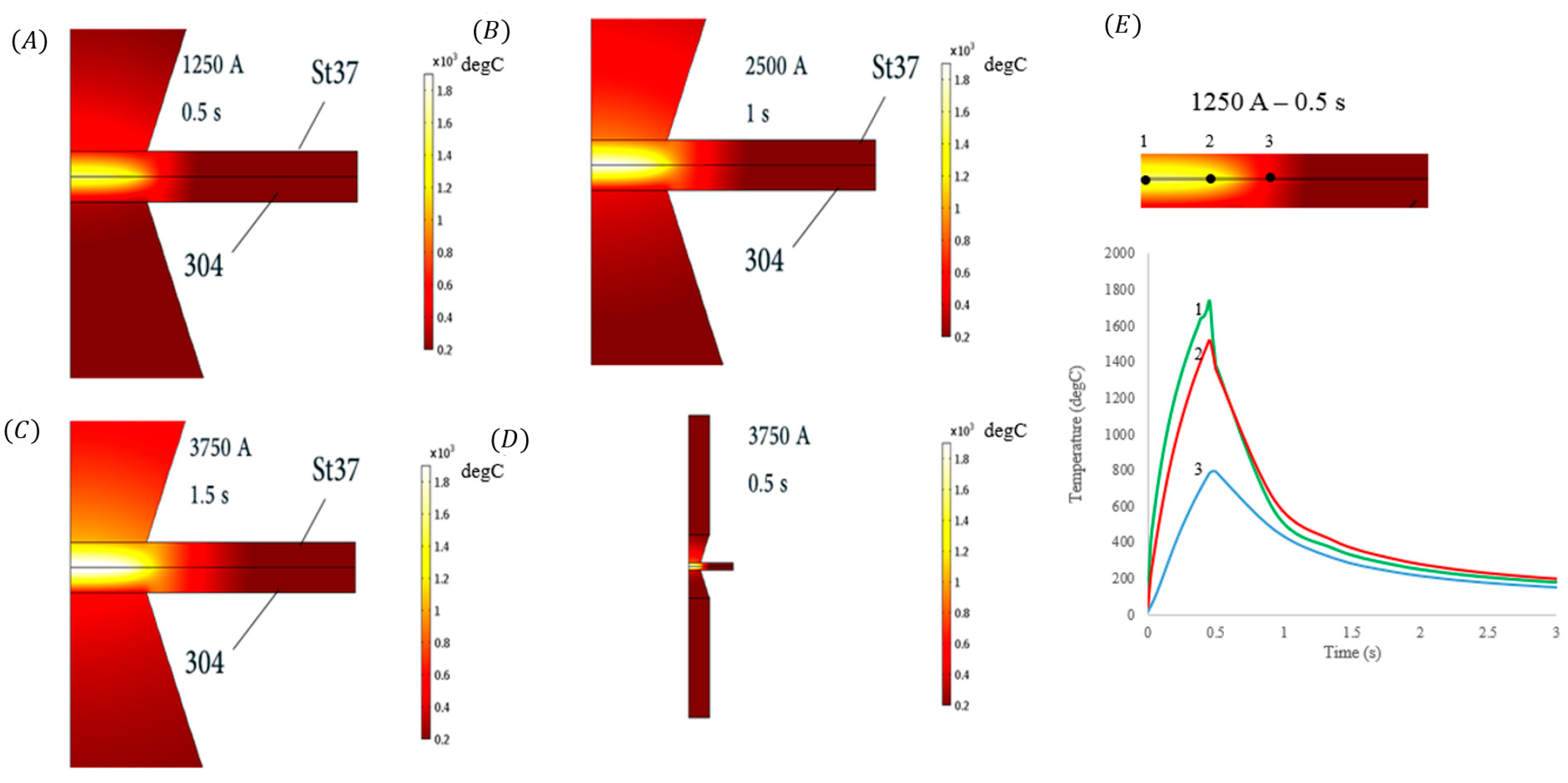
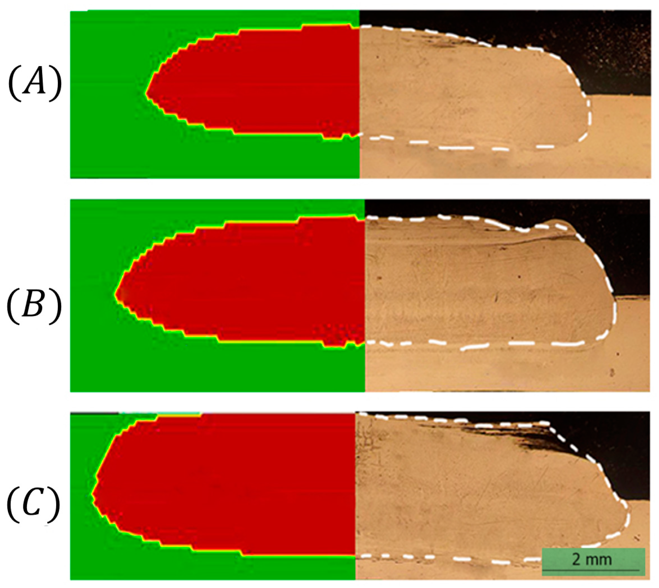
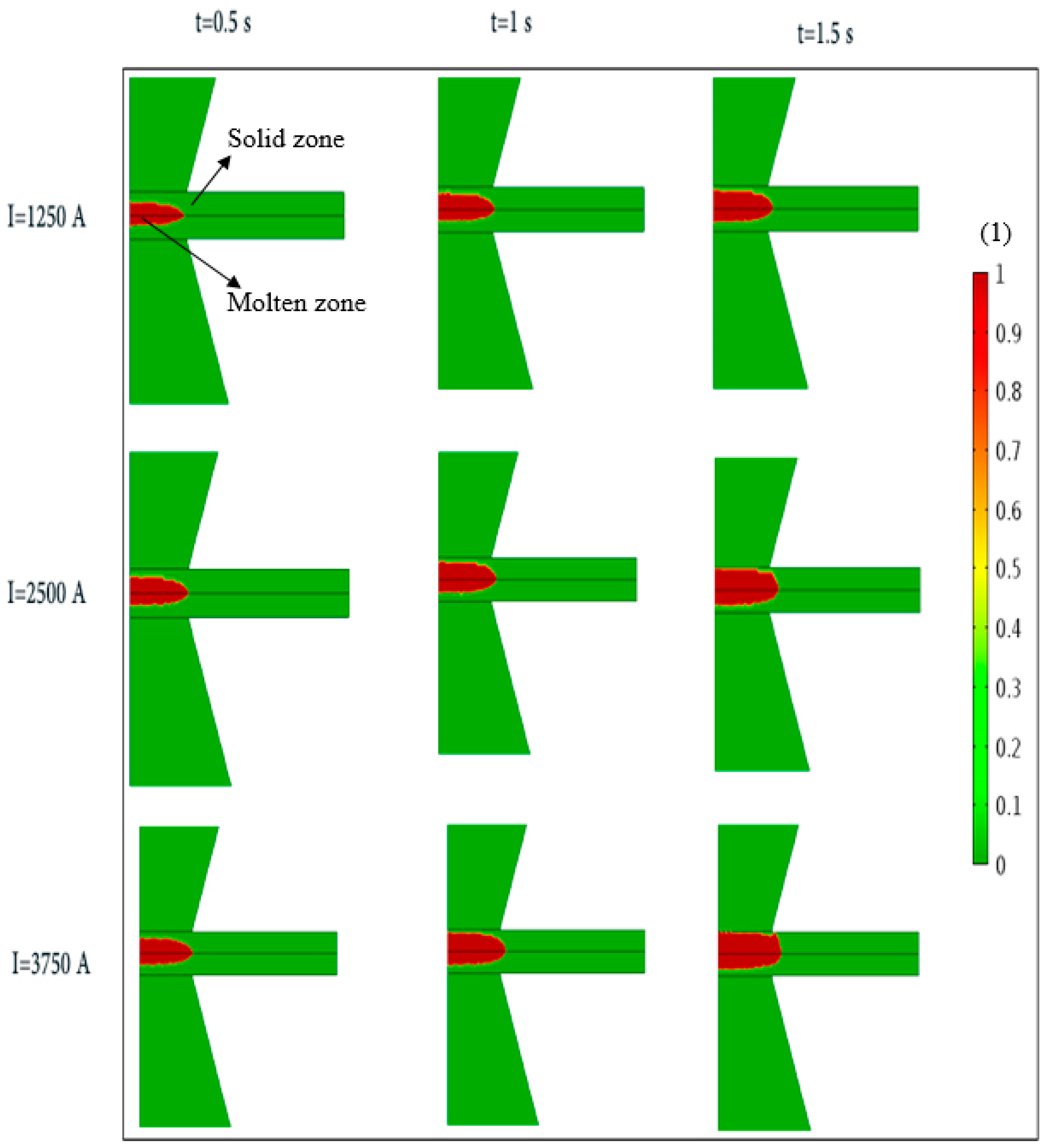
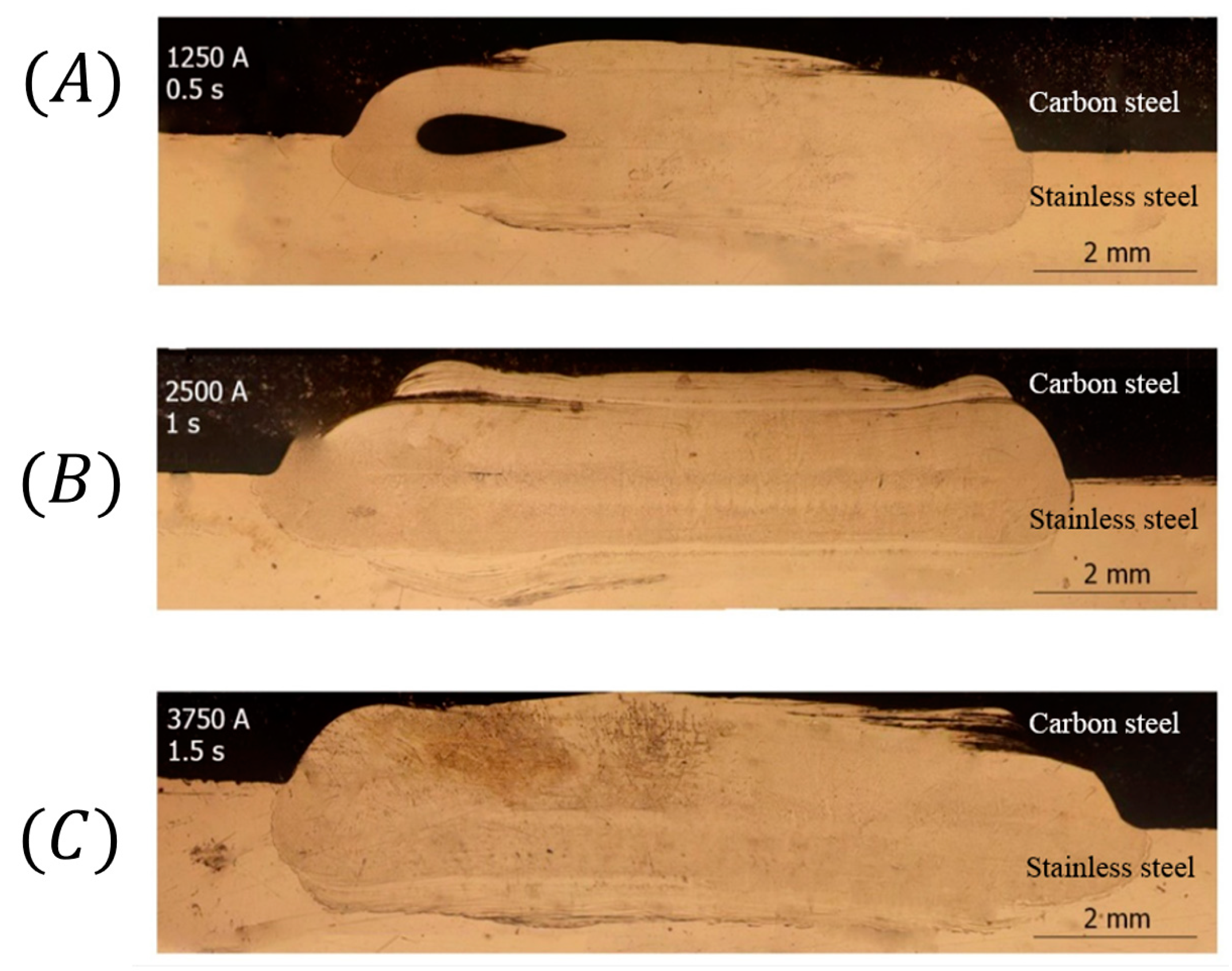
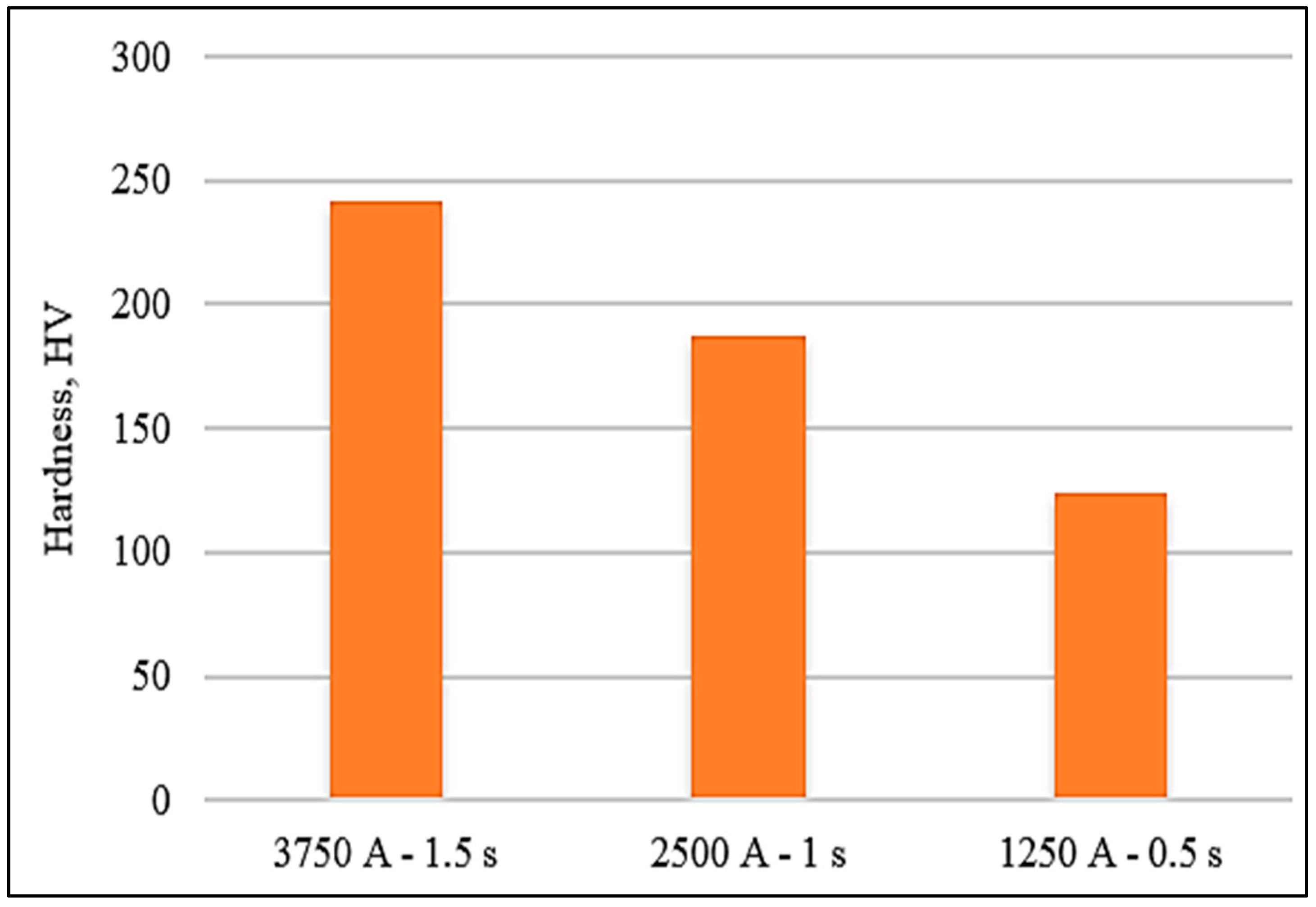
• Increasing the welding time (from 0.5 to 1.5 s) and current (from 1250 to 3750 degC) in the RSW process increases the heat input and consequently increases the diameter of the welding nugget.
• According to the proper agreement with negligible deviations of the experimental and simulation results, the FEM for solving the Laplace and Fourier equations is a suitable method for this process.
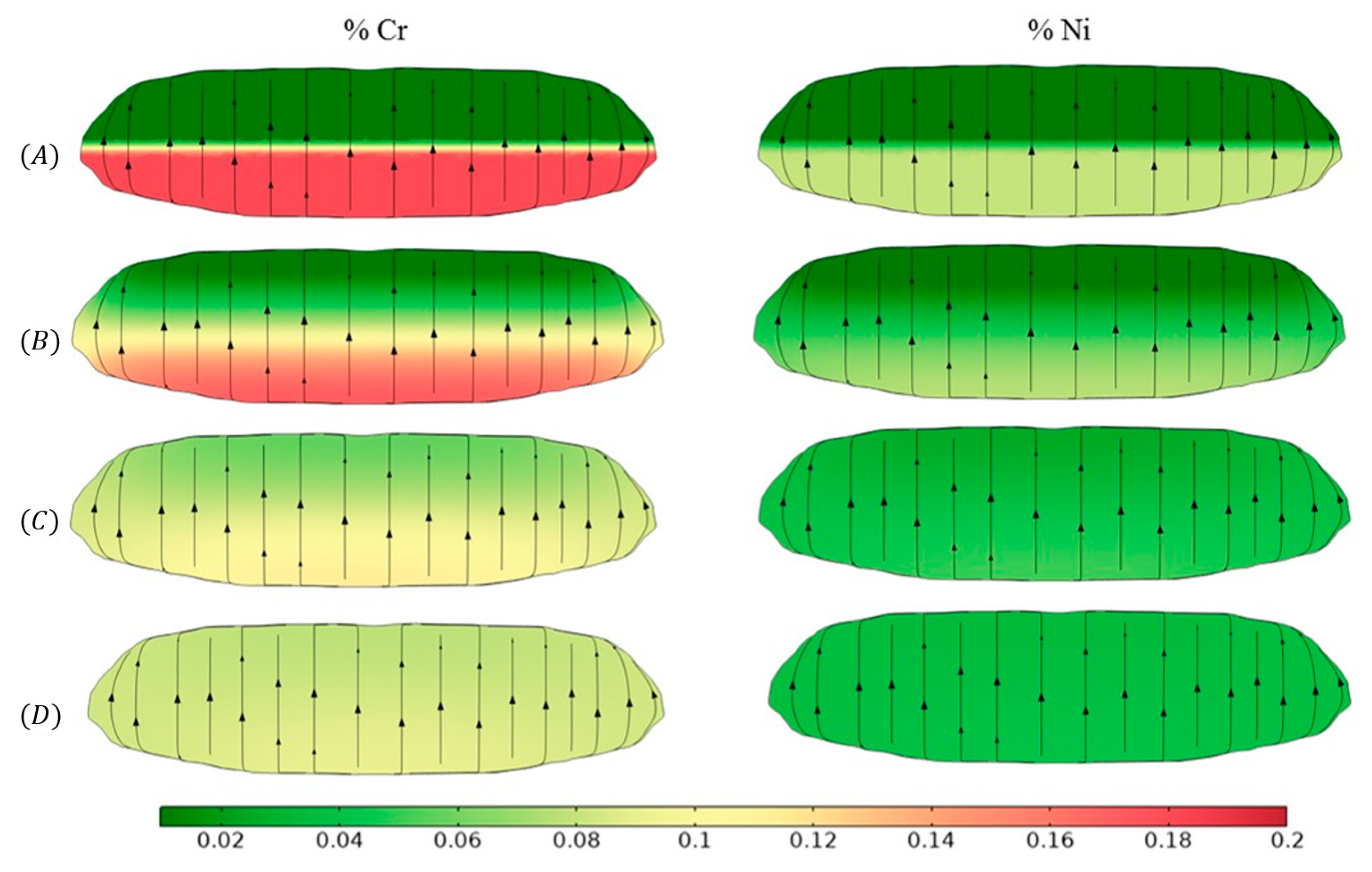
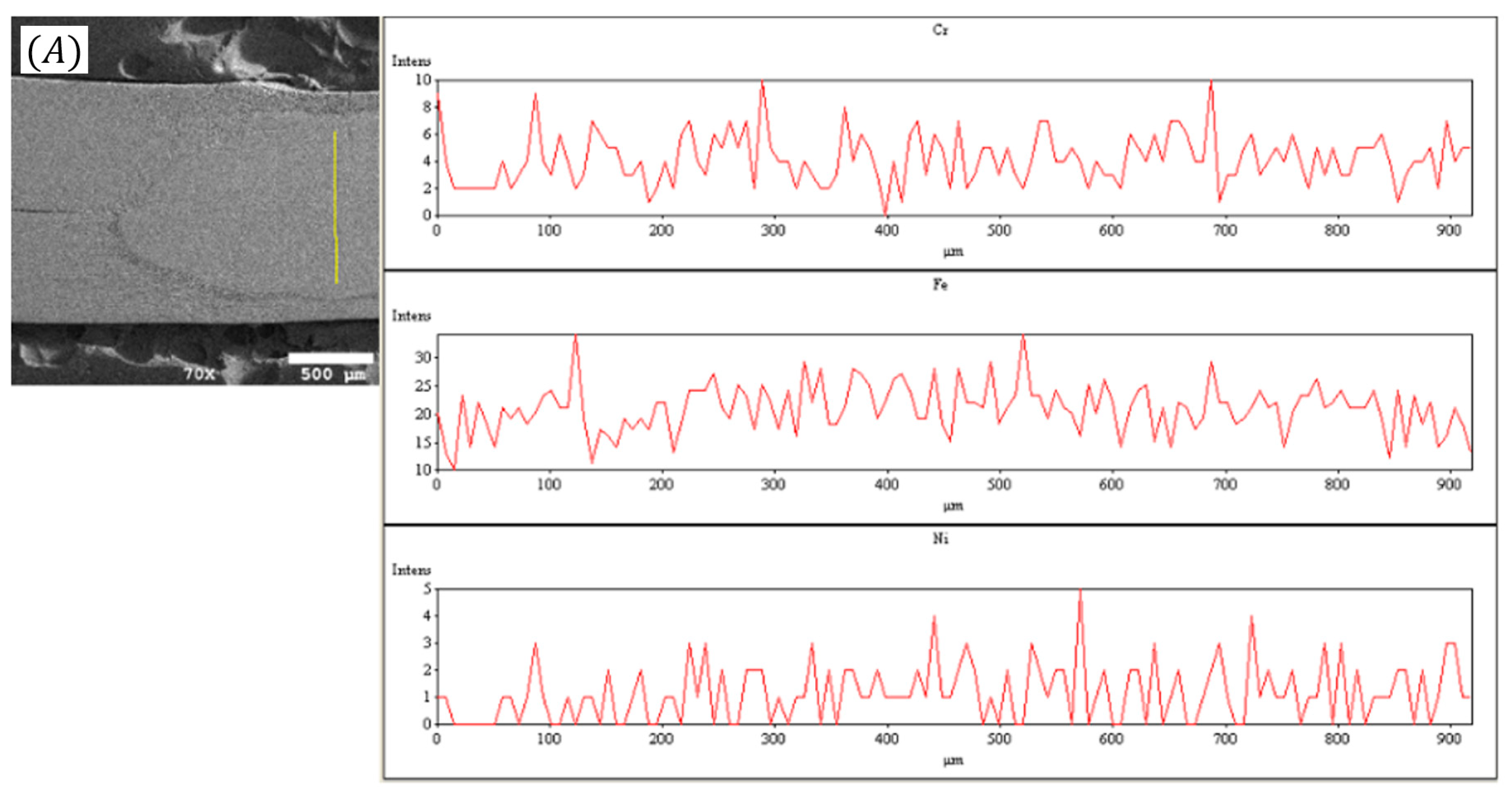
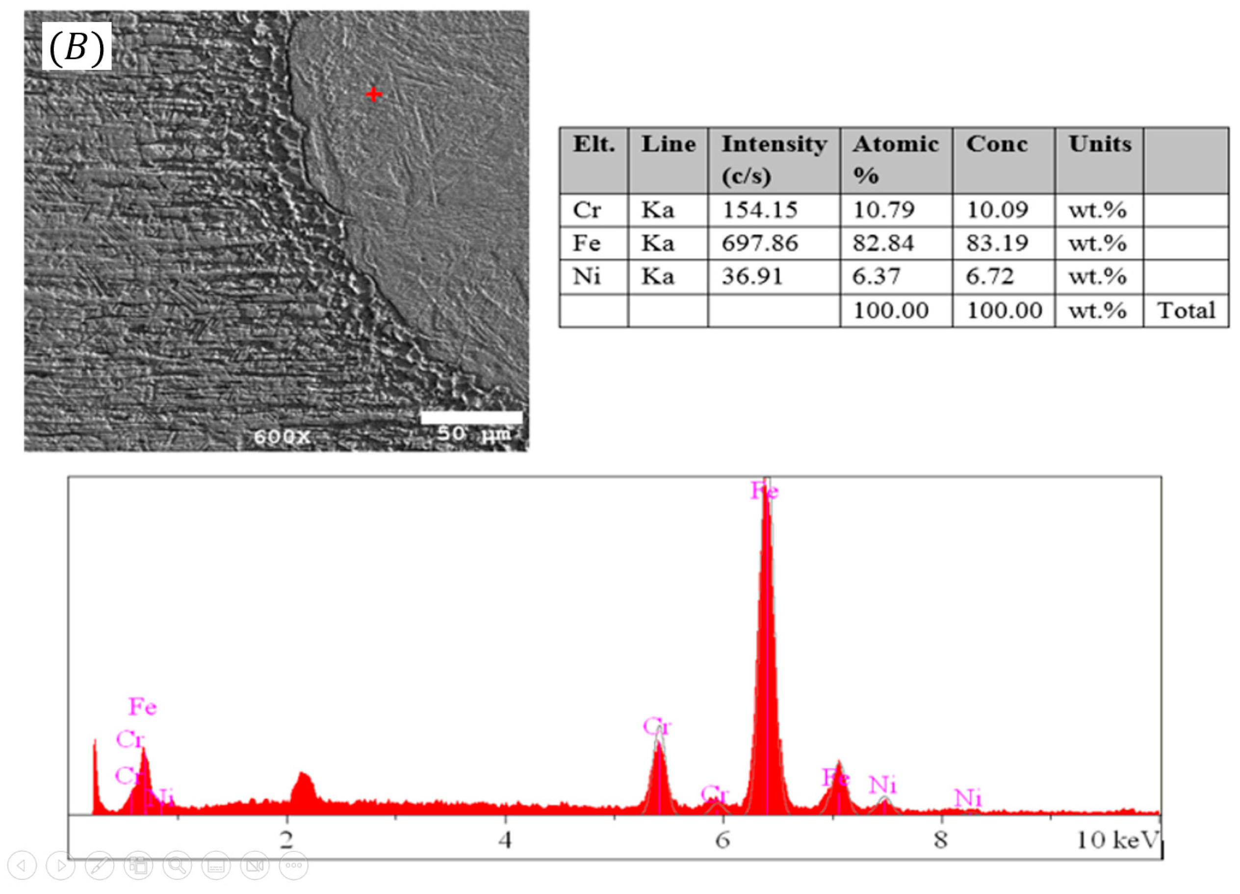
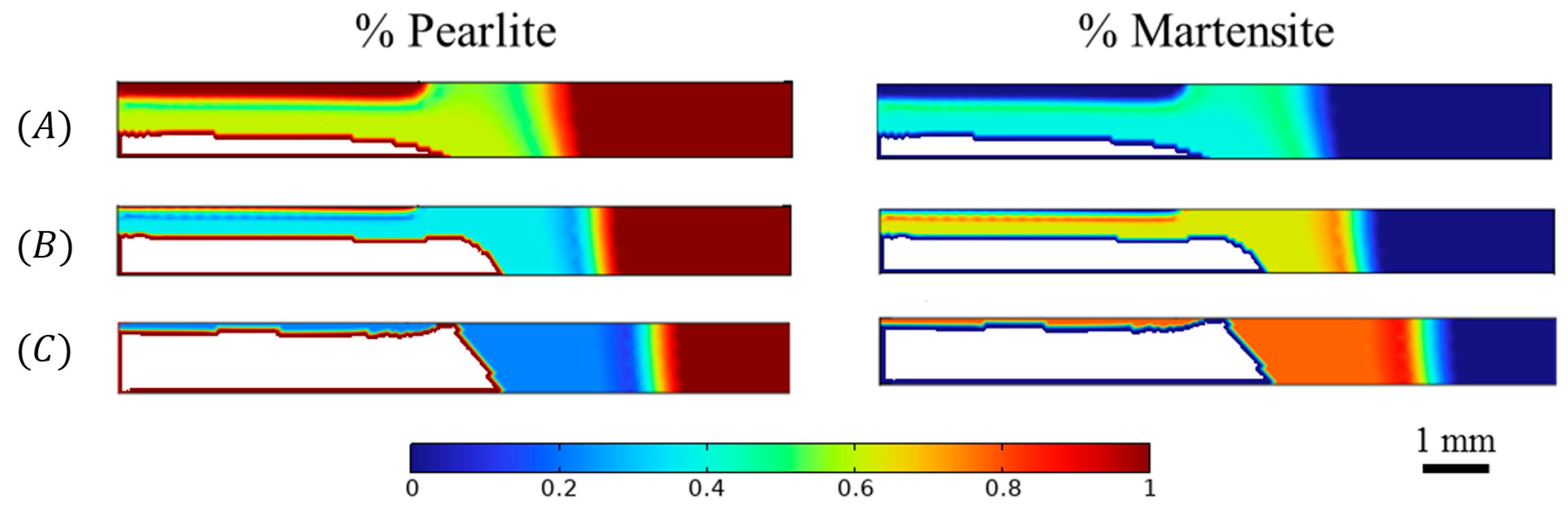
• Cr and Ni diffusion through the fusion zone, results in the formation of a kind of a stainless steel in the nugget zone. The simulated results was in consistence with experimental results.
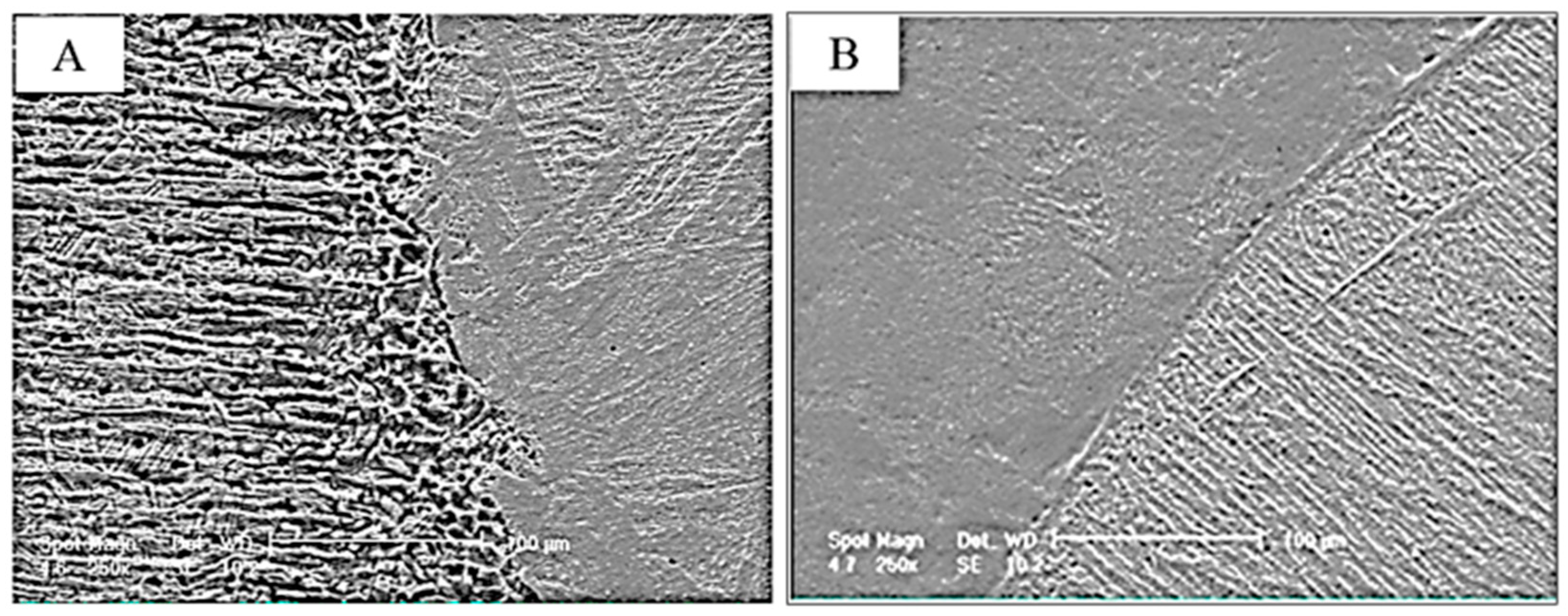
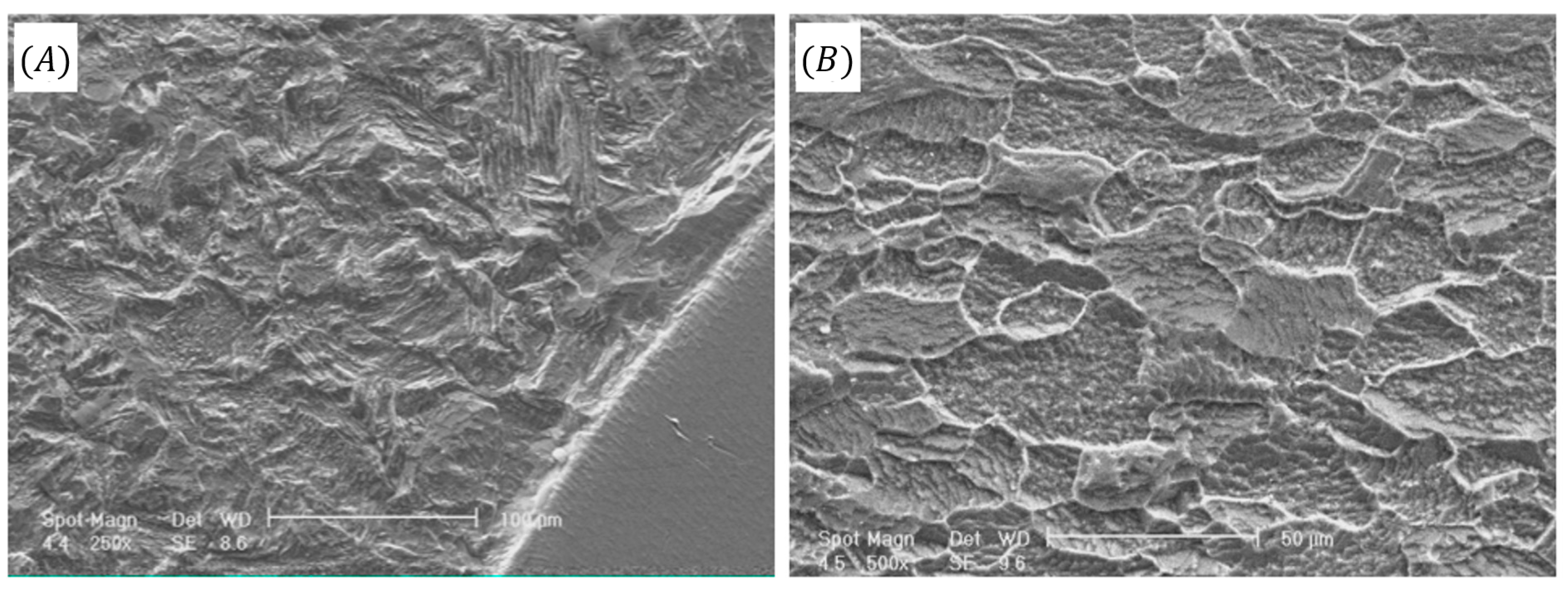
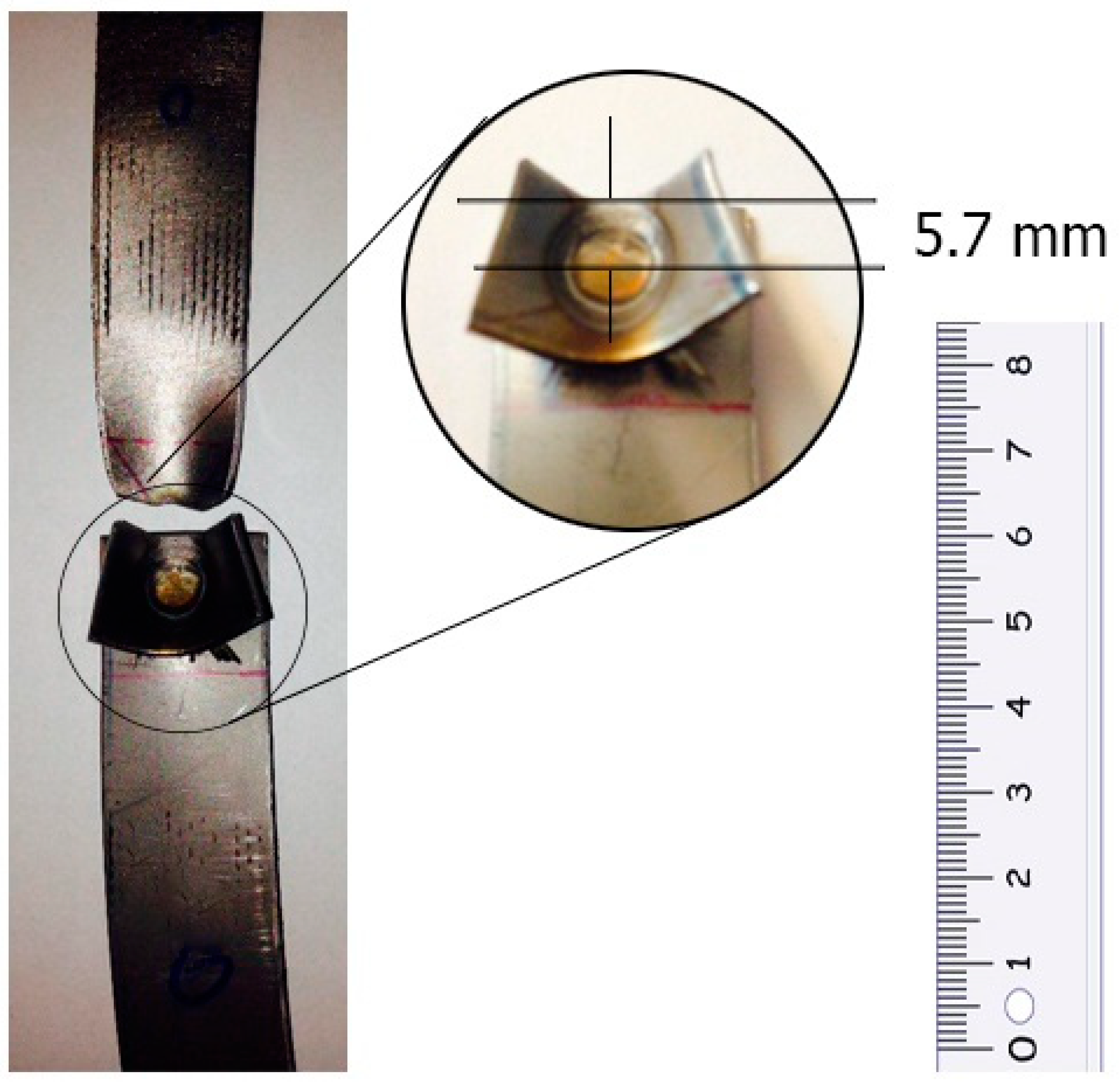
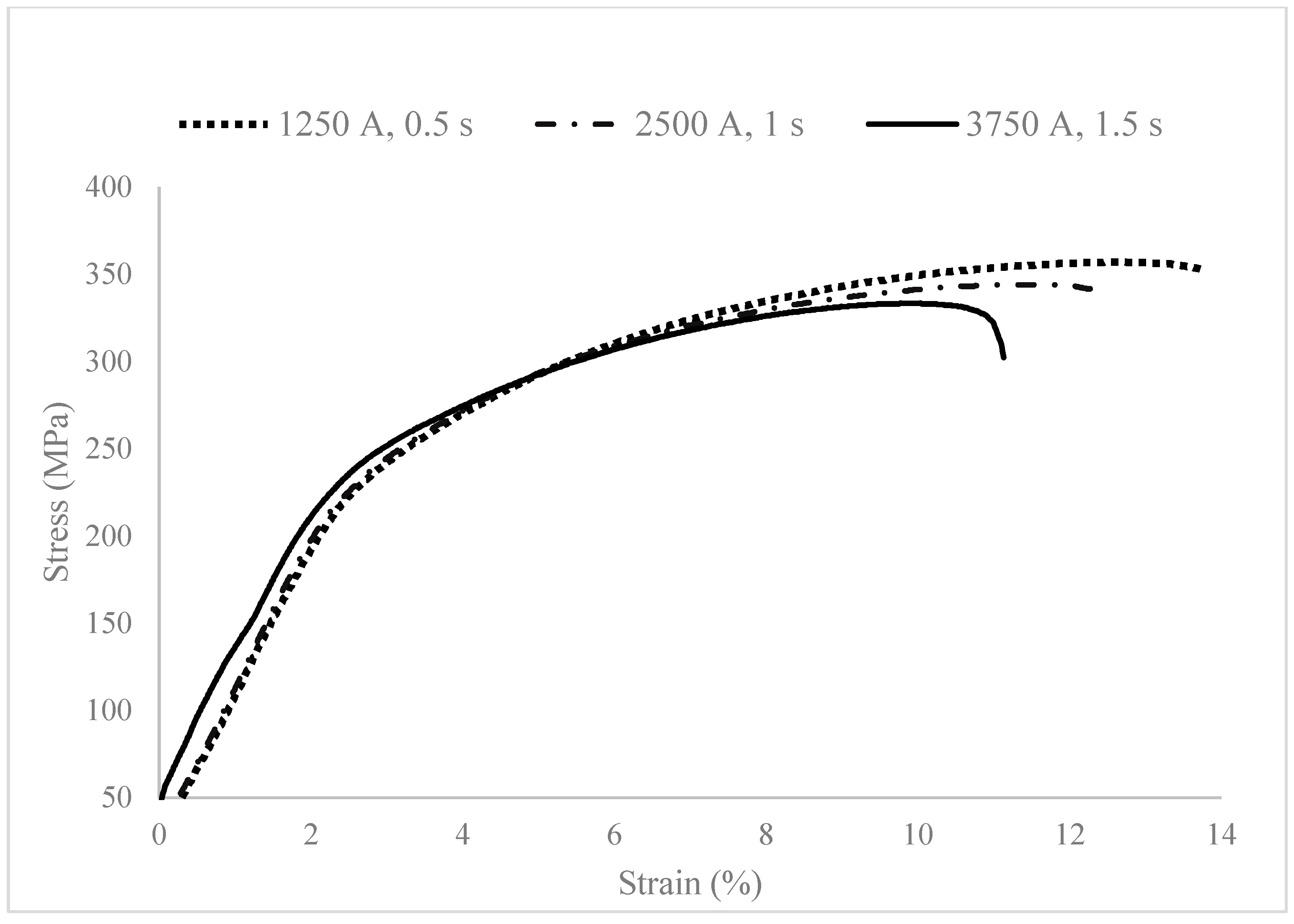
• The welding zone (weld nugget size) of stainless steel to carbon steel was so strong that all the specimens were broken from the carbon steel side in the tensile shear test. In fact, martensite formation in the HAZ results in more brittle region. This confirms the microstructure predictions.
• The results of microstructure prediction showed that increasing the heat input, including increasing the current and welding time, increases the percentage of martensite in the HAZ region and also widens the martensitic region, therefore, reduces the shear tensile strength.

References

1. Ul-Hamid, A.; Tawancy, H.M.; Abbas, N.M. Failure of weld joints between carbon steel pipe and 304 stainless steel elbows. Eng. Fail. Anal. 2005, 12, 181–191. [Google Scholar] [CrossRef]
2. Williams, N.; Parker, J. Review of resistance spot welding of steel sheets Part 1 Modelling and control of weld nugget formation. Int. Mater. Rev. 2004, 49, 45–75. [Google Scholar] [CrossRef]
3. Bag, S.; DiGiovanni, C.; Han, X.; Zhou, N.Y. A phenomenological model of resistance spot welding on liquid metal embrittlement severity using dynamic resistance measurement. J. Manuf. Sci. Eng. 2020, 142, 031007. [Google Scholar] [CrossRef]
4. Luo, Y.; Liu, J.; Xu, H.; Xiong, C.; Liu, L. Regression modeling and process analysis of resistance spot welding on galvanized steel sheet. Mater. Des. 2009, 30, 2547–2555. [Google Scholar] [CrossRef]
5. Muhammad, N.; Manurung, Y.H.P.; Jaafar, R.; Abas, S.K.; Tham, G.; Haruman, E. Model development for quality features of resistance spot welding using multi-objective Taguchi method and response surface methodology. J. Intell. Manuf. 2013, 24, 1175–1183. [Google Scholar] [CrossRef]
6. Martín, Ó.; López, M.; Martín, F. Artificial neural networks for quality control by ultrasonic testing in resistance spot welding. J. Mater. Process. Technol. 2007, 183, 226–233. [Google Scholar] [CrossRef]
7. Nied, H. The finite element modeling of the resistance spot welding process. Weld. J. 1984, 63, 123. [Google Scholar]
8. Browne, D.J.; Chandler, H.W.; Evans, J.T.; Wen, J. Computer simulation of resistance spot welding in aluminum: Part I. Weld. J.-Incl. Weld. Res. Suppl. 1995, 74, 339s. [Google Scholar]
9. Browne, D.J.; Chandler, H.W.; Evans, J.T.; James, P.S.; Wen, J.; Newton, C.J. Computer simulation of resistance spot welding in aluminum: Part II. Weld. J.-Incl. Weld. Res. Suppl. 1995, 74, 417s. [Google Scholar]
10. Wei, P.; Ho, C. Axisymmetric nugget growth during resistance spot welding. J. Heat Transfer. 1990, 112, 309–316. [Google Scholar] [CrossRef]
11. Gupta, O.; De, A. An improved numerical modeling for resistance spot welding process and its experimental verification. J. Manuf. Sci. Eng. 1998, 120, 246–251. [Google Scholar] [CrossRef]
12. Feng, Z. An incrementally couples electrical-thermal-mechanical model for resistance spot welding, trends in welding research. In Proceedings of the 5th International Conference on Trends in Welding Research, Pine Mountain, GA, USA, 1–5 June 1998; ASM International: Almere, The Netherlands. [Google Scholar]
13. Khan, J.; Xu, L.; Chao, Y.-J. Prediction of nugget development during resistance spot welding using coupled thermal–electrical–mechanical model. Sci. Technol. Weld. Join. 1999, 4, 201–207. [Google Scholar] [CrossRef]
14. Andersson, O.; Melander, A. Prediction and verification of resistance spot welding results of ultra-high strength steels through FE simulations. Model. Numer. Simul. Mater. Sci. 2015, 5, 26. [Google Scholar] [CrossRef]
15. Eisazadeh, H.; Hamedi, M.; Halvaee, A. New parametric study of nugget size in resistance spot welding process using finite element method. Mater. Des. 2010, 31, 149–157. [Google Scholar] [CrossRef]
16. Moshayedi, H.; Sattari-Far, I. Numerical and experimental study of nugget size growth in resistance spot welding of austenitic stainless steels. J. Mater. Process. Technol. 2012, 212, 347–354. [Google Scholar] [CrossRef]
17. Eshraghi, M.; Tschopp, M.A.; Zaeem, M.A.; Felicelli, S.D. Effect of resistance spot welding parameters on weld pool properties in a DP600 dual-phase steel: A parametric study using thermomechanically-coupled finite element analysis. Mater. Des. 2014, 56, 387–397. [Google Scholar] [CrossRef]
18. Wang, J.; Wang, H.-P.; Lu, F.; Carlson, B.E.; Sigler, D.R. Analysis of Al-steel resistance spot welding process by developing a fully coupled multi-physics simulation model. Int. J. Heat Mass Transf. 2015, 89, 1061–1072. [Google Scholar] [CrossRef]
19. Dancette, S.; Huin, T.; Dupuy, T.; Fabrègue, D. Finite element modeling of deformation and fracture of advanced high strength steels dissimilar spot welds. Eng. Fract. Mech. 2021, 258, 108092. [Google Scholar] [CrossRef]
20. Marashi, P.; Pouranvari, M.; Amirabdollahian, S.; Abedi, A.; Goodarzi, M. Microstructure and failure behavior of dissimilar resistance spot welds between low carbon galvanized and austenitic stainless steels. Mater. Sci. Eng. A 2008, 480, 175–180. [Google Scholar] [CrossRef]
21. Charde, N.; Yusof, F.; Rajkumar, R. Material characterizations of mild steels, stainless steels, and both steel mixed joints under resistance spot welding (2-mm sheets). Int. J. Adv. Manuf. Technol. 2014, 75, 373–384. [Google Scholar] [CrossRef]
22. Ishak, M.; Shah, L.H.; Aisha, I.S.R.; Hafizi, W.; Islam, M.R. Study of resistance spot welding between aisi 301 stainless steel and AISI 1020 carbon steel dissimilar alloys. J. Mech. Eng. Sci. 2014, 6, 793–806. [Google Scholar] [CrossRef]
23. Sani, M.; Nazri, N.; Alawi, D. Vibration analysis of resistance spot welding joint for dissimilar plate structure (mild steel 1010 and stainless steel 304). Proceeding of the IOP Conference Series: Materials Science and Engineering, Birmingham, UK, 13–15 October 2017; IOP Publishing: Bristol, UK, 2017. [Google Scholar]
24. Nandan, R.; Roy, G.G.; Lienert, T.J.; Debroy, T. Numerical modelling of 3D plastic flow and heat transfer during friction stir welding of stainless steel. Sci. Technol. Weld. Join. 2006, 11, 526–537. [Google Scholar] [CrossRef]
25. Nandan, R.; Roy, G.; Lienert, T.; Debroy, T. Three-dimensional heat and material flow during friction stir welding of mild steel. Acta Mater. 2007, 55, 883–895. [Google Scholar] [CrossRef]
26. McKee, R. A generalization of the Nernst-Einstein equation for self-diffusion in high defect concentration solids. Solid State Ion. 1981, 5, 133–136. [Google Scholar] [CrossRef] [Green Version]
27. Ono, Y.; Matsumoto, S. Diffusion of chromium, manganese, and nickel in molten iron. Trans. Jpn. Inst. Met. 1975, 16, 415–422. [Google Scholar] [CrossRef] [Green Version]
28. Leblond, J.; Devaux, J. A new kinetic model for anisothermal metallurgical transformations in steels including effect of austenite grain size. Acta Metall. 1984, 32, 137–146. [Google Scholar] [CrossRef]
29. Koistinen, D.P. A general equation prescribing the extent of the austenite-martensite transformation in pure iron-carbon alloys and plain carbon steels. Acta Metall. 1959, 7, 59–60. [Google Scholar] [CrossRef]
30. Leblond, J.-B.; Mottet, G.; Devaux, J.; Devaux, J.C. Mathematical models of anisothermal phase transformations in steels, and predicted plastic behaviour. Mater. Sci. Technol. 1985, 1, 815–822. [Google Scholar] [CrossRef]
31. Lan, L.; Qiu, C.; Song, H.; Zhao, D. Correlation of martensite–austenite constituent and cleavage crack initiation in welding heat affected zone of low carbon bainitic steel. Mater. Lett. 2014, 125, 86–88. [Google Scholar] [CrossRef]
Figure 1. Schematic of tensile shear test of samples.
Metals 12 01898 g001
Figure 2. Geometry, boundary conditions, and meshing of resistance spot welding model.
Metals 12 01898 g002
Figure 3. Simulation results of electrical potential distribution in the weld zone, (A) 1250 A and 0.5 s, (B) 2500 A and 1 s, (C) 3750 and 1.5 s, (D) electrodes 1250 A and 0.5 s.
Metals 12 01898 g003
Figure 4. Simulation results of electric current distribution in the weld zone, (A) 1250 A and 0.5 s, (B) 2500 A and 1 s, (C) 3750 and 1.5 s, (D) electrodes 1250 A and 0.5 s.
Metals 12 01898 g004
Figure 5. Simulation results of temperature distribution in the weld zone, (A) 1250 A and 0.5 s, (B) 2500 A and 1 s, (C) 3750 and 1.5 s, (D) electrodes 1250 A and 0.5 s and (E) is the thermal history diagram of three points in the weld zone and HAZ of 1250 A and 0.5 s specimen.
Metals 12 01898 g005
Figure 6. Evaluation of weld nugget simulation results with experimental results (A) 1250 A and 0.5 s, (B) 2500 A and 1 s, (C) 3750 and 1.5 s.
Metals 12 01898 g006
Figure 7. Simulation results of welding nugget size in the joint area during welding.
Metals 12 01898 g007
Figure 8. Macrostructure of the welding zone of dissimilar welding of 304 steel to carbon steel in different current and time conditions. (A) 1250 A and 0.5 s, (B) 2500 A and 1 s, (C) 3750 and 1.5 s.
Metals 12 01898 g008
Figure 9. Scanning electron microscopic images for the melting boundary with (A) 304 steel, (B) carbon steel.
Metals 12 01898 g009
Figure 10. Simulation results of Cr and Ni diffusion in the molten Fe, (A) 0.01 s, (B) 0.1 s, (C) 0.2 s, (D) 0.5 s.
Metals 12 01898 g010
Figure 11. (A) Linear EDS analysis of distribution of Fe, Cr and Ni elements in the weld zone, (B) point EDS analysis of weld nugget.
Metals 12 01898 g011aMetals 12 01898 g011b
Figure 12. Simulation results of martensite distribution in HAZ region, (A) 1250 A and 0.5 s, (B) 2500 A and 1 s, (C) 3750 and 1.5 s.
Metals 12 01898 g012
Figure 13. Scanning electron microscopy images of the (A) martensite phase region (B) pearlite-ferrite phase in HAZ carbon steel.
Metals 12 01898 g013
Figure 14. Micro-hardness values in HAZ of three different samples.
Metals 12 01898 g014
Figure 15. Fractured RSW sample during shear tensile test, 2500 A, 1 s.
Metals 12 01898 g015
Figure 16. Stress–strain diagram obtained from shear tensile test of samples welded by RSW method.
Metals 12 01898 g016