
Topological Optimization of Artificial Neural Networks to Estimate Mechanical Properties in Metal Forming Using Machine Learning


Abstract
:1. Introduction
2. Methodology
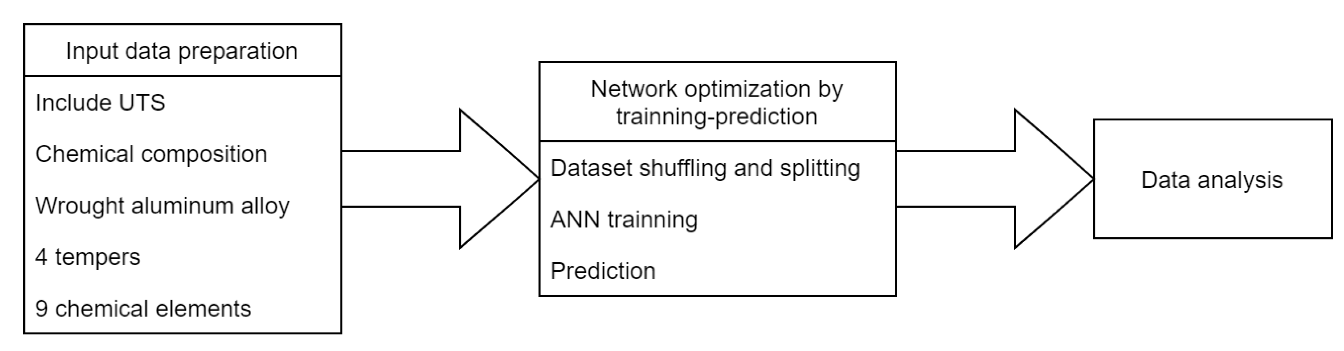
2.1. Input Dataset Preparation
- Only datasheets that contain the value of the ultimate tensile stress () at 20 °C are considered.
- Only alloys whose chemical composition is defined at more than are taken into account [13] (note that some datasheets are poorly defined).
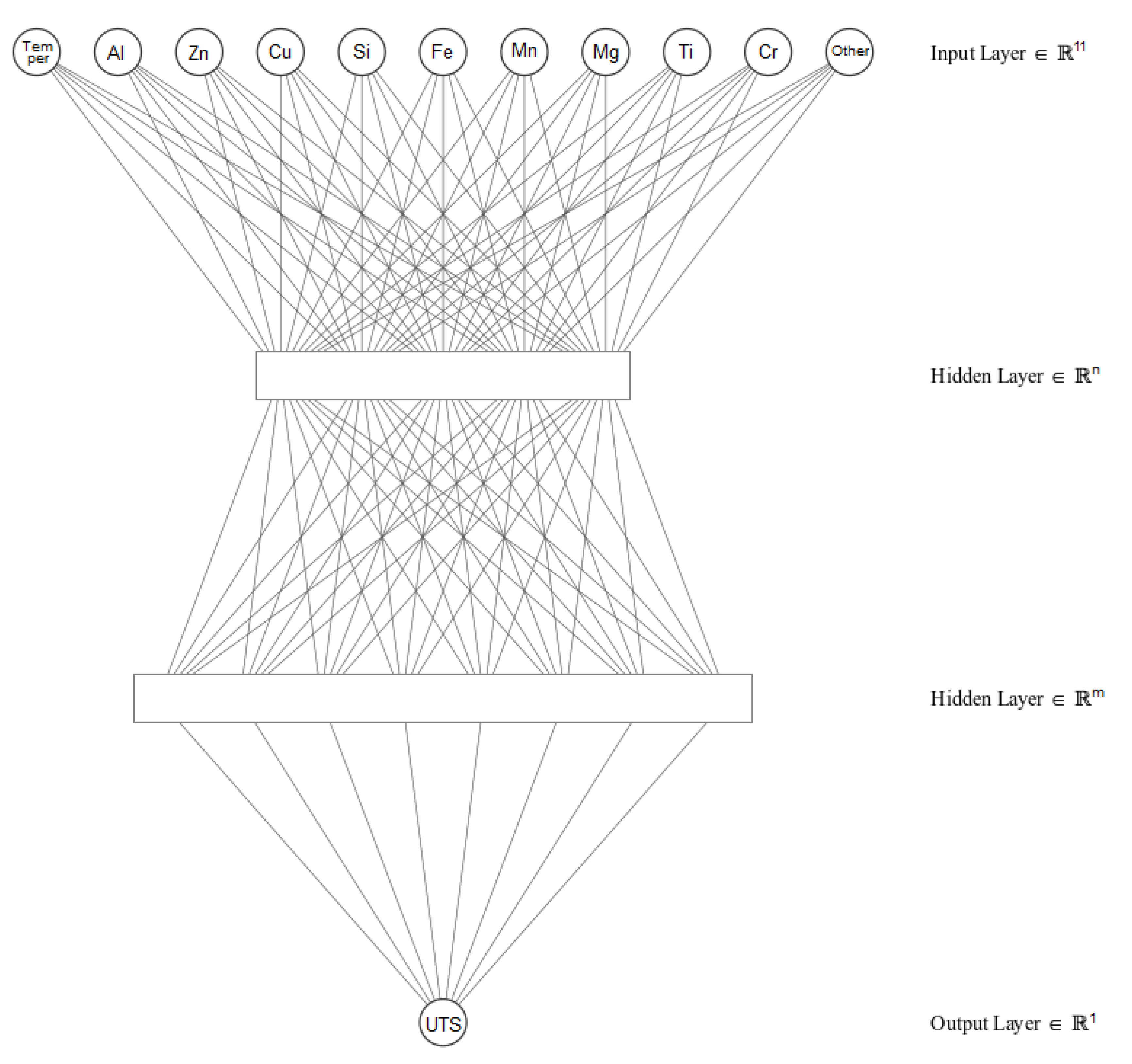
- Only 9 chemical elements are considered to define the chemical composition of the alloys [29]: Al, Zn, Cu, Si, Fe, Mn, Mg, Ti and Cr. The mass contribution of all other chemical elements is regrouped as ”Other”.
- Only wrought alloys are considered in this study.
- Only the specification sheets that include the temper of the alloy are considered. This study only considers the following tempers: F (as fabricated), O (annealed), H (strain hardening) and T (thermally treated) [7].
2.2. Network Optimization by Training-Prediction
- Dataset shuffling and splitting to create a training subset ( of records, so 2137) and a testing subset (remaining , so 534).
- ANN training, using the data contained in the training subset.
- Prediction of the properties for the records in the testing subset.
- Results and data storage for further analysis.
- Calculation of the learning rate for each parameter using adaptive moment estimation (ADAM) with , (algorithm parameters), (step size) and (stability factor) [36].
- Early stopping after 20 iterations without significant changes.
- Training stops when a training error of less than is reached.
- Maximum of 100,000 training epochs to avoid infinite loops.
2.3. Data Analysis
3. Results and Discussion
4. Conclusions and Future Work
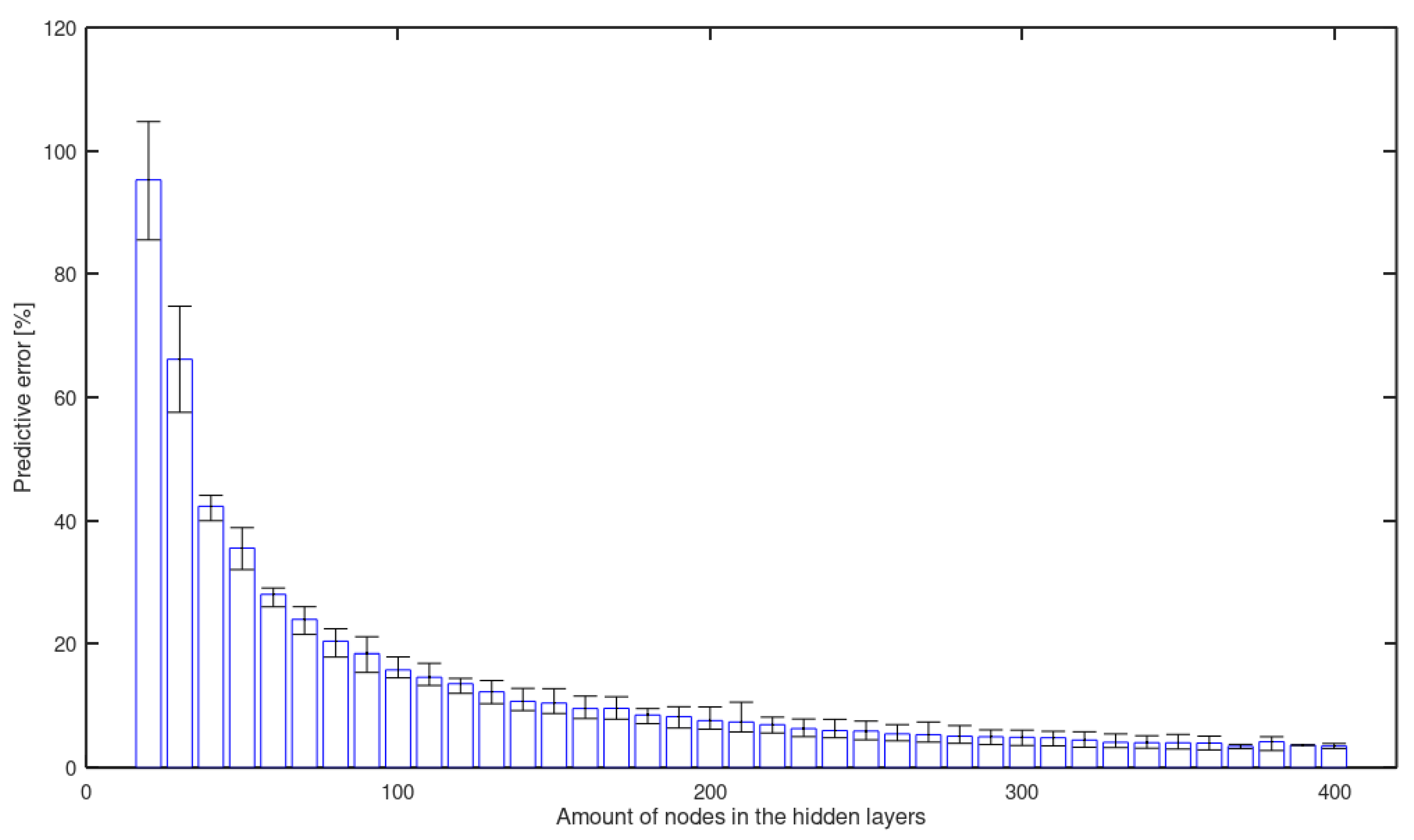
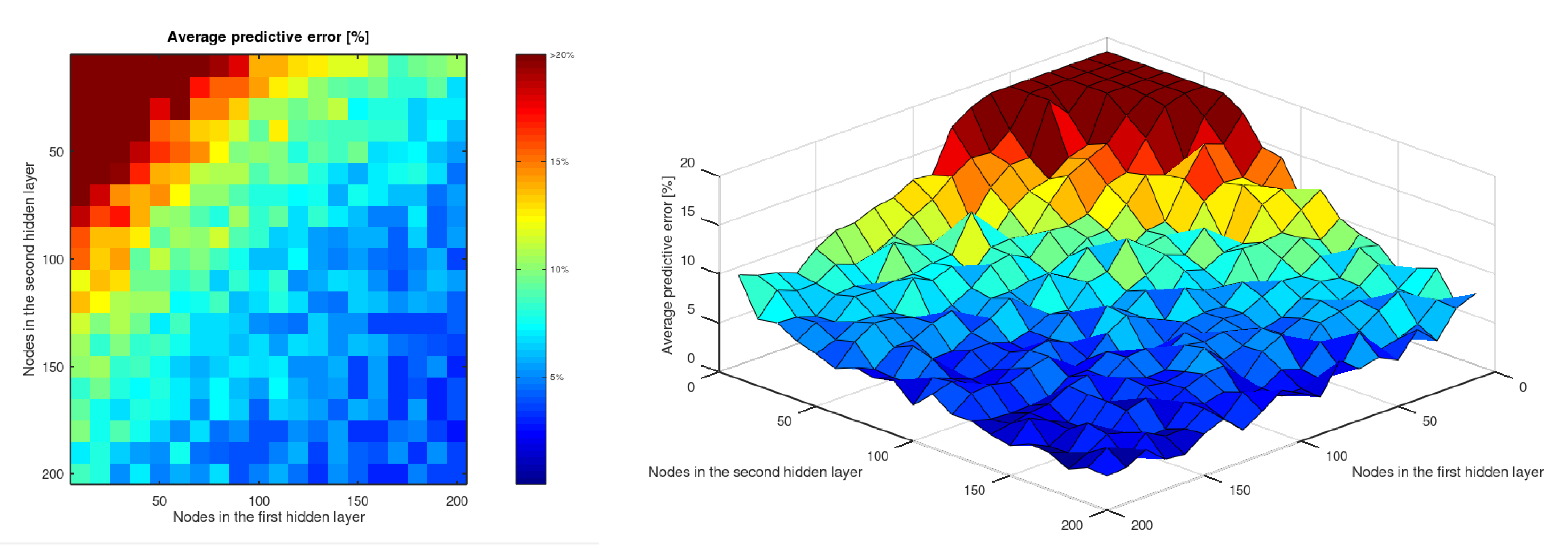
- An artificial neural network with two hidden layers can predict the of wrought aluminum alloys by taking its chemical composition and temper as input. The accuracy of this prediction stabilizes below and even reaches in this study.
- The predictive ability of an ANN with two hidden layers to estimate the of aluminum alloys is stabilized for topologies that include 150 or more perceptrons in both hidden layers. The precision and accuracy of these networks do not show significant differences that allow us to affirm that one topology is really better than the others.
- A multilayer ANN can be used as a tool to, through machine learning, make predictions about the mechanical behavior of a piece of aluminum alloy subjected to forming processes. In theory, these networks can learn to approximate any nonlinear function if the input data set is large enough and has enough perceptrons [37].
Author Contributions
Funding
Data Availability Statement
Acknowledgments
Conflicts of Interest
Abbreviations
| ADAM | Adaptive moment estimation |
| AI | Artificial intelligence |
| ANN | Artificial neural networks |
| ADAM algorithm parameter | |
| ADAM stability factor | |
| ADAM step size | |
| m | ADAM first moment estimate |
| ML | Machine learning |
| Ultimate tensile strength | |
| Standard deviation | |
| ADAM second moment estimate | |
| Average | |
| Yield strength |
Appendix A. Numerical Results

| Nodes in the First Hidden Layer | |||||||||||||||||||||
|---|---|---|---|---|---|---|---|---|---|---|---|---|---|---|---|---|---|---|---|---|---|
| 10 | 20 | 30 | 40 | 50 | 60 | 70 | 80 | 90 | 100 | 110 | 120 | 130 | 140 | 150 | 160 | 170 | 180 | 190 | 200 | ||
| Nodes in the second hidden layer | 10 | 95.28 | 74.79 | 44.11 | 34.89 | 28.74 | 23.07 | 20.56 | 19.26 | 17.96 | 13.79 | 13.98 | 12.86 | 12.55 | 11.70 | 11.60 | 10.48 | 8.68 | 9.42 | 9.86 | 10.62 |
| 20 | 57.57 | 39.99 | 36.42 | 29.08 | 22.67 | 21.50 | 16.95 | 15.34 | 15.52 | 14.29 | 12.68 | 11.64 | 10.31 | 9.29 | 8.84 | 9.57 | 8.33 | 8.30 | 9.07 | 6.79 | |
| 30 | 42.92 | 32.07 | 26.03 | 25.78 | 17.93 | 21.18 | 14.82 | 14.81 | 13.20 | 10.38 | 10.37 | 9.57 | 10.06 | 11.14 | 7.34 | 8.08 | 7.89 | 6.37 | 7.00 | 7.13 | |
| 40 | 38.87 | 28.11 | 21.55 | 20.78 | 15.44 | 14.82 | 13.33 | 12.82 | 11.55 | 9.26 | 12.81 | 9.13 | 9.02 | 8.56 | 8.56 | 8.27 | 8.43 | 6.51 | 7.19 | 5.98 | |
| 50 | 28.26 | 24.81 | 19.79 | 18.44 | 16.25 | 15.39 | 14.40 | 12.23 | 9.71 | 10.05 | 9.91 | 7.86 | 9.37 | 8.64 | 9.63 | 6.74 | 7.10 | 7.23 | 6.11 | 5.38 | |
| 60 | 26.05 | 22.47 | 19.38 | 16.83 | 14.03 | 13.50 | 11.19 | 10.70 | 10.86 | 8.80 | 9.88 | 9.54 | 7.88 | 6.84 | 5.93 | 6.97 | 7.58 | 7.84 | 6.62 | 4.57 | |
| 70 | 20.21 | 18.32 | 14.56 | 13.78 | 14.48 | 12.19 | 10.22 | 10.15 | 8.95 | 7.93 | 7.88 | 7.48 | 7.53 | 5.79 | 7.67 | 7.12 | 6.13 | 6.05 | 4.50 | 5.42 | |
| 80 | 18.73 | 16.20 | 16.92 | 14.03 | 10.41 | 10.17 | 8.79 | 7.96 | 10.60 | 8.24 | 9.34 | 6.65 | 8.23 | 6.88 | 6.14 | 4.94 | 4.89 | 6.91 | 4.35 | 5.01 | |
| 90 | 15.90 | 13.50 | 13.71 | 12.51 | 9.33 | 10.43 | 10.02 | 11.50 | 8.80 | 8.42 | 6.31 | 6.61 | 5.62 | 5.11 | 5.77 | 5.78 | 4.36 | 6.28 | 4.35 | 5.51 | |
| 100 | 15.52 | 13.30 | 14.13 | 9.33 | 11.15 | 9.13 | 9.85 | 8.45 | 7.53 | 6.23 | 5.99 | 7.45 | 5.54 | 4.87 | 5.55 | 4.41 | 4.20 | 4.94 | 5.77 | 3.66 | |
| 110 | 12.05 | 13.74 | 12.86 | 9.58 | 9.39 | 8.33 | 8.94 | 6.42 | 8.33 | 6.91 | 8.19 | 5.26 | 5.82 | 6.77 | 6.43 | 5.26 | 3.94 | 5.08 | 6.09 | 5.51 | |
| 120 | 13.69 | 12.34 | 10.69 | 10.43 | 10.48 | 7.33 | 7.60 | 8.60 | 6.01 | 6.86 | 7.89 | 6.78 | 4.87 | 4.39 | 6.54 | 6.04 | 5.30 | 5.77 | 5.57 | 4.12 | |
| 130 | 11.45 | 9.94 | 10.87 | 9.45 | 7.13 | 8.46 | 6.68 | 6.78 | 6.49 | 5.03 | 4.85 | 4.52 | 6.30 | 5.10 | 5.17 | 3.74 | 3.60 | 3.54 | 3.66 | 4.19 | |
| 140 | 10.57 | 8.26 | 9.72 | 8.36 | 8.62 | 7.70 | 6.71 | 6.83 | 6.01 | 6.82 | 5.56 | 6.65 | 6.45 | 5.09 | 6.05 | 5.63 | 4.51 | 4.30 | 3.89 | 3.49 | |
| 150 | 10.13 | 10.59 | 8.20 | 8.53 | 7.54 | 6.26 | 5.77 | 6.43 | 6.93 | 6.59 | 6.98 | 5.13 | 5.06 | 5.76 | 3.64 | 5.47 | 3.31 | 4.23 | 5.18 | 3.08 | |
| 160 | 8.28 | 9.58 | 8.06 | 7.28 | 7.99 | 6.88 | 6.05 | 7.30 | 6.21 | 5.48 | 7.41 | 5.68 | 5.27 | 5.62 | 3.54 | 5.48 | 3.28 | 4.06 | 3.02 | 3.96 | |
| 170 | 9.19 | 7.77 | 6.65 | 7.98 | 7.59 | 7.16 | 5.01 | 7.28 | 6.32 | 4.14 | 6.29 | 6.13 | 5.38 | 4.24 | 5.82 | 5.23 | 3.31 | 5.39 | 3.03 | 3.78 | |
| 180 | 9.88 | 7.68 | 8.91 | 7.66 | 6.36 | 5.04 | 6.65 | 4.53 | 5.18 | 3.98 | 3.78 | 5.03 | 4.53 | 5.42 | 3.35 | 3.15 | 4.41 | 4.95 | 3.74 | 2.77 | |
| 190 | 7.01 | 8.05 | 6.31 | 5.50 | 5.01 | 7.55 | 4.65 | 4.24 | 3.95 | 3.89 | 4.87 | 5.72 | 3.72 | 5.47 | 4.10 | 4.05 | 5.12 | 3.22 | 5.01 | 3.64 | |
| 200 | 8.72 | 7.92 | 5.30 | 7.15 | 4.74 | 5.73 | 5.26 | 6.82 | 3.79 | 4.90 | 5.90 | 4.45 | 3.25 | 5.07 | 4.27 | 2.88 | 3.07 | 4.81 | 3.67 | 3.49 | |
| Nodes in the First Hidden Layer | |||||||||||||||||||||
|---|---|---|---|---|---|---|---|---|---|---|---|---|---|---|---|---|---|---|---|---|---|
| 10 | 20 | 30 | 40 | 50 | 60 | 70 | 80 | 90 | 100 | 110 | 120 | 130 | 140 | 150 | 160 | 170 | 180 | 190 | 200 | ||
| Nodes in the second hidden layer | 10 | 58.96 | 28.75 | 61.09 | 41.95 | 13.42 | 23.40 | 6.31 | 9.94 | 14.81 | 13.57 | 13.25 | 13.00 | 12.76 | 3.60 | 3.21 | 5.28 | 5.72 | 5.05 | 4.87 | 4.62 |
| 20 | 19.33 | 47.56 | 13.39 | 16.32 | 8.62 | 18.35 | 6.16 | 5.14 | 7.12 | 11.86 | 4.15 | 5.40 | 8.93 | 8.26 | 3.32 | 2.75 | 5.08 | 8.61 | 2.39 | 3.99 | |
| 30 | 22.01 | 16.41 | 26.93 | 10.95 | 22.21 | 17.56 | 8.28 | 4.40 | 12.88 | 4.23 | 10.87 | 4.80 | 8.39 | 8.28 | 8.64 | 2.87 | 6.43 | 7.93 | 2.21 | 2.53 | |
| 40 | 17.07 | 31.23 | 24.15 | 20.37 | 8.87 | 7.79 | 6.70 | 6.03 | 3.40 | 3.28 | 3.88 | 4.19 | 11.49 | 4.30 | 2.86 | 7.13 | 2.30 | 3.65 | 3.23 | 7.03 | |
| 50 | 9.52 | 11.56 | 9.35 | 7.92 | 6.87 | 6.95 | 6.25 | 5.54 | 5.34 | 9.62 | 4.03 | 7.33 | 8.89 | 3.87 | 6.29 | 6.88 | 3.23 | 2.39 | 3.70 | 4.72 | |
| 60 | 22.65 | 10.43 | 7.95 | 4.66 | 4.46 | 12.15 | 12.45 | 9.26 | 11.20 | 3.04 | 2.95 | 3.99 | 8.77 | 8.28 | 2.87 | 2.18 | 7.99 | 3.06 | 3.33 | 2.24 | |
| 70 | 22.05 | 18.31 | 4.78 | 13.17 | 12.53 | 4.21 | 4.64 | 10.87 | 5.03 | 4.91 | 2.94 | 3.79 | 2.70 | 6.73 | 3.78 | 5.19 | 7.10 | 1.97 | 6.82 | 4.71 | |
| 80 | 17.48 | 21.58 | 4.26 | 6.41 | 6.29 | 3.91 | 5.55 | 5.11 | 3.36 | 3.97 | 2.53 | 4.49 | 1.90 | 2.50 | 2.32 | 1.78 | 5.58 | 1.82 | 2.17 | 1.97 | |
| 90 | 17.69 | 16.30 | 4.24 | 12.62 | 9.19 | 5.24 | 10.07 | 2.52 | 4.04 | 2.64 | 7.91 | 3.56 | 1.94 | 2.66 | 2.29 | 2.82 | 2.84 | 6.09 | 1.79 | 5.04 | |
| 100 | 4.50 | 12.01 | 4.13 | 12.25 | 11.17 | 7.81 | 4.86 | 8.29 | 7.72 | 3.51 | 6.66 | 3.55 | 7.05 | 2.39 | 1.64 | 1.47 | 2.65 | 3.20 | 3.82 | 1.23 | |
| 110 | 6.31 | 11.91 | 9.64 | 4.32 | 5.36 | 4.71 | 2.59 | 6.47 | 6.06 | 7.08 | 2.10 | 3.62 | 2.27 | 2.59 | 2.23 | 2.13 | 2.02 | 4.48 | 1.26 | 3.52 | |
| 120 | 5.57 | 11.89 | 2.95 | 8.35 | 7.60 | 2.90 | 3.01 | 2.70 | 6.68 | 1.82 | 3.50 | 4.76 | 5.99 | 4.37 | 2.14 | 5.54 | 4.87 | 2.35 | 4.48 | 1.12 | |
| 130 | 3.80 | 9.36 | 8.35 | 9.85 | 7.08 | 3.39 | 3.90 | 6.64 | 5.35 | 2.09 | 1.59 | 5.57 | 1.44 | 1.84 | 2.71 | 1.92 | 2.39 | 1.19 | 1.79 | 1.70 | |
| 140 | 11.68 | 2.80 | 4.81 | 8.22 | 2.50 | 3.56 | 3.93 | 3.52 | 2.45 | 5.78 | 5.55 | 4.94 | 4.24 | 3.92 | 2.51 | 1.89 | 3.45 | 4.52 | 4.18 | 1.53 | |
| 150 | 10.64 | 3.94 | 3.58 | 7.68 | 7.39 | 2.30 | 2.57 | 6.58 | 3.49 | 6.99 | 7.12 | 2.16 | 2.55 | 4.93 | 1.68 | 1.18 | 4.50 | 2.60 | 4.16 | 2.29 | |
| 160 | 3.19 | 9.65 | 7.71 | 6.33 | 8.70 | 5.79 | 3.60 | 2.45 | 1.63 | 2.27 | 2.08 | 1.52 | 3.94 | 4.45 | 1.37 | 1.44 | 1.59 | 1.05 | 1.70 | 2.45 | |
| 170 | 5.24 | 9.33 | 3.48 | 3.42 | 3.28 | 7.52 | 3.63 | 2.18 | 3.25 | 4.41 | 3.99 | 3.95 | 2.81 | 2.44 | 3.32 | 3.50 | 5.10 | 2.95 | 1.34 | 2.77 | |
| 180 | 10.02 | 3.72 | 2.33 | 4.27 | 6.64 | 5.74 | 5.60 | 2.10 | 6.98 | 5.18 | 1.97 | 1.55 | 1.77 | 5.35 | 1.63 | 2.55 | 4.05 | 1.94 | 1.59 | 1.90 | |
| 190 | 2.29 | 2.30 | 3.78 | 5.29 | 2.60 | 7.36 | 2.21 | 2.18 | 2.72 | 5.01 | 4.60 | 5.89 | 1.78 | 2.59 | 1.07 | 4.19 | 2.14 | 4.17 | 4.71 | 1.38 | |
| 200 | 2.83 | 2.29 | 5.43 | 7.18 | 6.58 | 2.21 | 1.55 | 3.09 | 2.05 | 1.21 | 2.77 | 5.38 | 5.40 | 1.64 | 2.58 | 2.01 | 1.48 | 2.00 | 2.62 | 1.74 | |
References
- Merayo, D.; Rodríguez-Prieto, A.; Camacho, A.M. Prediction of the Bilinear Stress-Strain Curve of Aluminum Alloys Using Artificial Intelligence and Big Data. Metals 2020, 10, 904. [Google Scholar] [CrossRef]
- Alam, T.; Ansari, A.H. Review on Aluminium and Its Alloys for automotive applications. Int. J. Adv. Technol. Eng. Sci. 2017, 5, 278–294. [Google Scholar]
- Merayo, D.; Rodríguez-Prieto, A.; Camacho, A.M. Prediction of mechanical properties by artificial neural networks to characterize the plastic behavior of aluminum alloys. Materials 2020, 13, 5227. [Google Scholar] [CrossRef]
- Ashkenazi, D. How aluminum changed the world: A metallurgical revolution through technological and cultural perspectives. Technol. Forecast. Soc. Chang. 2019, 143, 101–113. [Google Scholar] [CrossRef]
- Hahn, G.; Rosenfield, A. Metallurgical factors affecting fracture toughness of aluminum alloys. Metall. Trans. A 1975, 6, 653–668. [Google Scholar] [CrossRef]
- Yogo, Y.; Sawamura, M.; Iwata, N.; Yukawa, N. Stress-strain curve measurements of aluminum alloy and carbon steel by unconstrained-type high-pressure torsion testing. Mater. Des. 2017, 122, 226–235. [Google Scholar] [CrossRef]
- Kaufman, J.G. Introduction to Aluminum Alloys and Tempers; ASM international: Russell Township, Geauga County, OH, USA, 2000. [Google Scholar]
- Kamaya, M.; Kawakubo, M. A procedure for determining the true stress–strain curve over a large range of strains using digital image correlation and finite element analysis. Mech. Mater. 2011, 43, 243–253. [Google Scholar] [CrossRef]
- Hu, J.; Marciniak, Z.; Duncan, J. Mechanics of Sheet Metal Forming; Elsevier: Amsterdam, The Netherlands, 2002. [Google Scholar]
- Hosford, W.F.; Caddell, R.M. Metal Forming: Mechanics and Metallurgy; Cambridge University Press: Cambridge, UK, 2011. [Google Scholar]
- Zhao, Y.; Song, B.; Pei, J.; Jia, C.; Li, B.; Linlin, G. Effect of deformation speed on the microstructure and mechanical properties of AA6063 during continuous extrusion process. J. Mater. Process. Technol. 2013, 213, 1855–1863. [Google Scholar] [CrossRef]
- Ilyas, M.; Hussain, G.; Rashid, H.; Alkahtani, M. Influence of Forming Parameters on the Mechanical Behavior of a Thin Aluminum Sheet Processed through Single Point Incremental Forming. Metals 2020, 10, 1461. [Google Scholar] [CrossRef]
- Merayo, D.; Rodríguez-Prieto, A.; Camacho, A.M. Prediction of Physical and Mechanical Properties for Metallic Materials Selection Using Big Data and Artificial Neural Networks. IEEE Access 2020, 8, 13444–13456. [Google Scholar] [CrossRef]
- Ghosh, I.; Das, S.K.; Chakraborty, N. An artificial neural network model to characterize porosity defects during solidification of A356 aluminum alloy. Neural Comput. Appl. 2014, 25, 653–662. [Google Scholar] [CrossRef]
- Zhao, D.; Ren, D.; Zhao, K.; Pan, S.; Guo, X. Effect of welding parameters on tensile strength of ultrasonic spot welded joints of aluminum to steel–By experimentation and artificial neural network. J. Manuf. Process. 2017, 30, 63–74. [Google Scholar] [CrossRef]
- Haghdadi, N.; Zarei-Hanzaki, A.; Khalesian, A.; Abedi, H. Artificial neural network modeling to predict the hot deformation behavior of an A356 aluminum alloy. Mater. Des. 2013, 49, 386–391. [Google Scholar] [CrossRef]
- Huang, J.; Liew, J.; Ademiloye, A.; Liew, K. Artificial intelligence in materials modeling and design. Arch. Comput. Methods Eng. 2020, 28, 3399–3413. [Google Scholar] [CrossRef]
- Jordan, M.I.; Mitchell, T.M. Machine learning: Trends, perspectives, and prospects. Science 2015, 349, 255–260. [Google Scholar] [CrossRef]
- Merayo, D.; Rodriguez-Prieto, A.; Camacho, A.M. Comparative analysis of artificial intelligence techniques for material selection applied to manufacturing in Industry 4.0. Procedia Manuf. 2019, 41, 42–49. [Google Scholar] [CrossRef]
- Jackson, P.C. Introduction to Artificial Intelligence; Courier Dover Publications: Mineola, NY, USA, 2019. [Google Scholar]
- Chen, C.T.; Gu, G.X. Machine learning for composite materials. MRS Commun. 2019, 9, 556–566. [Google Scholar] [CrossRef] [Green Version]
- Joshi, P. Artificial Intelligence with Python; Packt Publishing Ltd.: Birmingham, UK, 2017. [Google Scholar]
- Dimiduk, D.M.; Holm, E.A.; Niezgoda, S.R. Perspectives on the impact of machine learning, deep learning, and artificial intelligence on materials, processes, and structures engineering. Integr. Mater. Manuf. Innov. 2018, 7, 157–172. [Google Scholar] [CrossRef] [Green Version]
- Balachandran, P.V.; Xue, D.; Theiler, J.; Hogden, J.; Gubernatis, J.E.; Lookman, T. Importance of feature selection in machine learning and adaptive design for materials. In Materials Discovery and Design; Springer: Berlin/Heidelberg, Germany, 2018; pp. 59–79. [Google Scholar]
- Feng, S.; Zhou, H.; Dong, H. Using deep neural network with small dataset to predict material defects. Mater. Des. 2019, 162, 300–310. [Google Scholar] [CrossRef]
- Mueller, T.; Kusne, A.G.; Ramprasad, R. Machine learning in materials science: Recent progress and emerging applications. Rev. Comput. Chem. 2016, 29, 186–273. [Google Scholar]
- Lefik, M.; Boso, D.; Schrefler, B. Artificial neural networks in numerical modelling of composites. Comput. Methods Appl. Mech. Eng. 2009, 198, 1785–1804. [Google Scholar] [CrossRef]
- Sha, W.; Edwards, K. The use of artificial neural networks in materials science based research. Mater. Des. 2007, 28, 1747–1752. [Google Scholar] [CrossRef]
- Davis, J.R. Alloying: Understanding the Basics; ASM International: Russell Township, Geauga County, OH, USA, 2001. [Google Scholar]
- Naik, D.L.; Sajid, H.U.; Kiran, R. Texture-based metallurgical phase identification in structural steels: A supervised machine learning approach. Metals 2019, 9, 546. [Google Scholar] [CrossRef] [Green Version]
- Honysz, R. Modeling the Chemical Composition of Ferritic Stainless Steels with the Use of Artificial Neural Networks. Metals 2021, 11, 724. [Google Scholar] [CrossRef]
- Qian, L.; Winfree, E.; Bruck, J. Neural network computation with DNA strand displacement cascades. Nature 2011, 475, 368–372. [Google Scholar] [CrossRef]
- Schmidhuber, J. Deep learning in neural networks: An overview. Neural Netw. 2015, 61, 85–117. [Google Scholar] [CrossRef] [PubMed] [Green Version]
- The Aluminum Association. Designations and Chemical Composition Limits for Aluminum Alloys in the Form of Castings and Ingot; The Aluminum Association Inc.: Arlington, VA, USA, 2006. [Google Scholar]
- Matmatch GmbH. Matmatch. 2021. Available online: https://matmatch.com/ (accessed on 15 June 2021).
- Kingma, D.; Ba, J. Adam: A method for stochastic optimization. In Proceedings of the 3rd International Conference for Learning Representations (ICLR 15), San Diego, CA, USA, 7–9 May 2015. [Google Scholar]
- Hornik, K. Approximation capabilities of multilayer feedforward networks. Neural Netw. 1991, 4, 251–257. [Google Scholar] [CrossRef]


| [] | Al [%] | Zn [%] | Cu [%] | Si [%] | Fe [%] | Mn [%] | Mg [%] | Ti [%] | Cr [%] | Other [%] | |
|---|---|---|---|---|---|---|---|---|---|---|---|
| Average | 246.3 | 95.1 | 0.6 | 1.0 | 0.5 | 0.5 | 0.5 | 1.4 | 0.2 | 0.2 | 0.2 |
| Std. dev. | 115.1 | 2.6 | 1.3 | 1.6 | 0.6 | 0.2 | 0.4 | 1.4 | 0.2 | 0.1 | 0.3 |
| Median | 230.0 | 95.9 | 0.3 | 0.3 | 0.4 | 0.5 | 0.5 | 0.9 | 0.1 | 0.1 | 0.0 |
| Min. | 40.0 | 83.1 | 0.0 | 0.0 | 0.0 | 0.0 | 0.0 | 0.0 | 0.0 | 0.0 | 0.0 |
| Max. | 700.0 | 99.7 | 7.8 | 6.3 | 12.3 | 1.6 | 1.6 | 5.5 | 0.8 | 0.9 | 2.0 |
Publisher’s Note: MDPI stays neutral with regard to jurisdictional claims in published maps and institutional affiliations. |
© 2021 by the authors. Licensee MDPI, Basel, Switzerland. This article is an open access article distributed under the terms and conditions of the Creative Commons Attribution (CC BY) license (https://creativecommons.org/licenses/by/4.0/).
Share and Cite
Merayo, D.; Rodríguez-Prieto, A.; Camacho, A.M. Topological Optimization of Artificial Neural Networks to Estimate Mechanical Properties in Metal Forming Using Machine Learning. Metals 2021, 11, 1289. https://doi.org/10.3390/met11081289
Merayo D, Rodríguez-Prieto A, Camacho AM. Topological Optimization of Artificial Neural Networks to Estimate Mechanical Properties in Metal Forming Using Machine Learning. Metals. 2021; 11(8):1289. https://doi.org/10.3390/met11081289
Chicago/Turabian StyleMerayo, David, Alvaro Rodríguez-Prieto, and Ana María Camacho. 2021. "Topological Optimization of Artificial Neural Networks to Estimate Mechanical Properties in Metal Forming Using Machine Learning" Metals 11, no. 8: 1289. https://doi.org/10.3390/met11081289
APA StyleMerayo, D., Rodríguez-Prieto, A., & Camacho, A. M. (2021). Topological Optimization of Artificial Neural Networks to Estimate Mechanical Properties in Metal Forming Using Machine Learning. Metals, 11(8), 1289. https://doi.org/10.3390/met11081289