Article

Seismic Collapse Risk Assessment of Braced Frames under Near-Fault Earthquakes

Department of Civil and Environmental Engineering, Colorado State University, Fort Collins, CO 80523, USA
*
Author to whom correspondence should be addressed.
Metals 2021, 11(8), 1271; https://doi.org/10.3390/met11081271
Submission received: 27 June 2021 / Revised: 2 August 2021 / Accepted: 7 August 2021 / Published: 11 August 2021
(This article belongs to the Special Issue Sustainable and Resilient Steel Structures)

Abstract

:
Special concentrically braced frames (SCBFs) located in regions close to earthquake faults may be subjected to near-fault ground motions, often characterized by pulses with long periods. These near-fault pulses could impose additional seismic demands on structures and increase the risk for structural collapse. Currently, there is limited research on the seismic collapse risk of SCBFs under near-fault earthquakes. This paper uses a general simulation-based framework to assess the seismic collapse risk of SCBFs under near-fault earthquakes. To quantify the large variability and uncertainty associated with the seismic hazard, a stochastic ground motion (SGM) model is used where the near-fault pulse characteristics are explicitly incorporated. The uncertainties in the SGM model parameters (including the near-fault pulse characteristics) are addressed through appropriate selection of probability distribution functions. To accurately predict the occurrence of collapse, numerical models capable of capturing the nonlinear and collapse behavior are established and used. Efficient stochastic simulation approaches are proposed to estimate the seismic collapse risk with or without considering the near-fault pulse. As an illustration, the seismic collapse risks of two SCBFs are investigated and compared. Probabilistic sensitivity analysis is also carried out to investigate the importance of uncertain model parameters within the SGM towards the seismic collapse risk.

1. Introduction

One of the most crucial objectives of the building codes is life safety, which is ensured by protecting structures against collapse under seismic events. With the advancement in earthquake engineering, the concept of performance-based earthquake engineering has gained popularity, which considers the entire range of seismic structural behaviors, including nonlinear behavior up to collapse. Standard performance levels put forward by the Applied Technology Council [1] and Federal Emergency Management Agency [2] include operational, immediate occupancy, life safety, and collapse prevention. Collapse prevention is the performance level where the structure may experience large damage to the structural components without collapsing. Although the design methodology is meant to prevent morbidity, significant social and economic losses could be expected [3]. In regions with high seismicity, special moment resisting frames (SMRF) were considered a viable option as lateral load-resisting systems for buildings; however, earthquakes such as the 1994 Northridge earthquake, 1995 Hyogo-Ken Nanbu earthquake, and other recent earthquakes, led to brittle fractures in many beam-to-column connections, compromising the integrity of such systems. The more extensive guidelines and restrictions related to the design of SMRFs have led to a shift towards investigating simplistic yet economical lateral resisting systems for low and mid-rise buildings, and concentrically braced frames (CBFs) became a favorable choice for seismic load-resisting systems [4].
CBFs are one of the most economical lateral load-resisting systems for low-rise structures, which utilize truss members connected concentrically at beam-to-column joints. The system provides high stiffness and strength but tends to have low ductility, which hinders the system’s ability to maintain the overall strength under severe earthquakes. Due to low ductility, the yielding members may experience low or ultra-low cycle fatigue under seismic loading. This issue can be resolved by utilizing a special class of CBFs called special concentrically braced frames (SCBFs) where the members that are expected to yield are carefully designed and detailed to achieve higher ductility during inelastic deformations [5]. Studies have been conducted to understand the behavior of braces connected to gusset plates [6,7,8,9,10,11] and the overall system performance. These studies resulted in improvements to the design and connection detailing that improved the overall performance of the system by further extending the ductility of the SCBFs.
To realize the full potential of SCBFs, an assessment of system response under both and far-field and near-fault ground motions should be conducted. There are many studies on the behavior of SCBFs subjected to far-field earthquakes [4,5,11,12]; however, assessment of the viability of SCBFs to near-field earthquakes has not received similar attention. Structures located in regions close to earthquake faults may be subjected to near-fault earthquakes. Near-fault ground motions, often characterized by forward directivity pulses with long periods, can impose additional and higher seismic demands on structures, which could increase the likelihood for unpredictable damages, brittle fracture, or low and ultra-low cycle fatigue of structural components, and even collapse [13]. While the performance of different structures under near-fault earthquakes have been investigated by different researchers [6,13,14,15,16,17,18,19], overall there is limited research on the seismic collapse risk of SCBFs under near-fault earthquakes and the impacts of near-fault earthquakes on braced frames, especially the collapse risk, are still not well understood.
To assess the seismic collapse performance of structures, usually incremental dynamic analysis (IDA) is used. In IDA nonlinear time history analysis of the structure is carried out under a set of selected recorded ground motions, and these ground motions are scaled up until the engineering demand parameters (EDPs) go through the entire range of behavior, from elastic to inelastic and finally to global dynamic instability [20,21]. IDA can be used to develop fragility curves for the damage state of collapse [22,23], which represents the probability of collapse under a given intensity measures and can be further used to estimate seismic collapse risk by propagating the uncertainties in the intensity measures. Though helpful in assessing collapse performance, the use of scaled ground motion in IDA raises concerns. For example, there is the concern on the validity of scaled ground motions, which may not represent actual ground motions (e.g., in terms of frequency contents and other characteristics). In addition, typically, ground motions with near-fault pulse are not explicitly considered due to the scarcity of recorded near-fault ground motions. In the context of seismic collapse risk assessment under near-fault earthquakes, the variability in the ground motions may not be properly quantified. Moreover, how the seismic hazard characteristics and near-fault pulse characteristics impact the seismic collapse risk is still not well understood. These challenges hinder better understanding of seismic collapse performance and the risk of structures close to earthquake faults. A better understanding of such risk can guide the continued improvement of the building codes and design philosophies.
To investigate the seismic collapse risk of SCBFs under near-fault earthquakes, this study used a general simulation-based framework, which facilitates the adoption of complex models and the consideration of various sources of uncertainties associated with the structure and the seismic hazards. To quantify the large variability and uncertainty associated with the seismic hazard, a stochastic ground motion (SGM) model was used to generate synthetic ground motions. The near-fault pulse characteristics were explicitly incorporated in the SGM model. The uncertainties in the SGM model parameters (including the near-fault pulse characteristics) were addressed through appropriate selection of probability distribution functions (PDFs). To accurately predict the occurrence of collapse, numerical models capable of capturing the nonlinear and collapse behavior were established and used in nonlinear time history analysis subject to the stochastic ground motion excitations. An efficient stochastic simulation was proposed to estimate the seismic collapse risk under near-fault earthquakes. An efficient approach using Bayes’ theorem was developed to directly calculate the seismic collapse risk when the near-fault pulse is neglected without running additional simulations. As an illustration, the seismic collapse risk of two typical SCBFs (i.e., SCBF with chevron bracing and SCBF with cross bracing) were investigated. Probabilistic sensitivity analysis was carried out to investigate the importance of each (or groups of) uncertain model parameters within the SGM including the near-fault pulse characteristics towards the seismic collapse risk of the two example braced frames.

2. Quantification of Seismic Collapse Risk of Braced Frames under Near-Fault Earthquakes

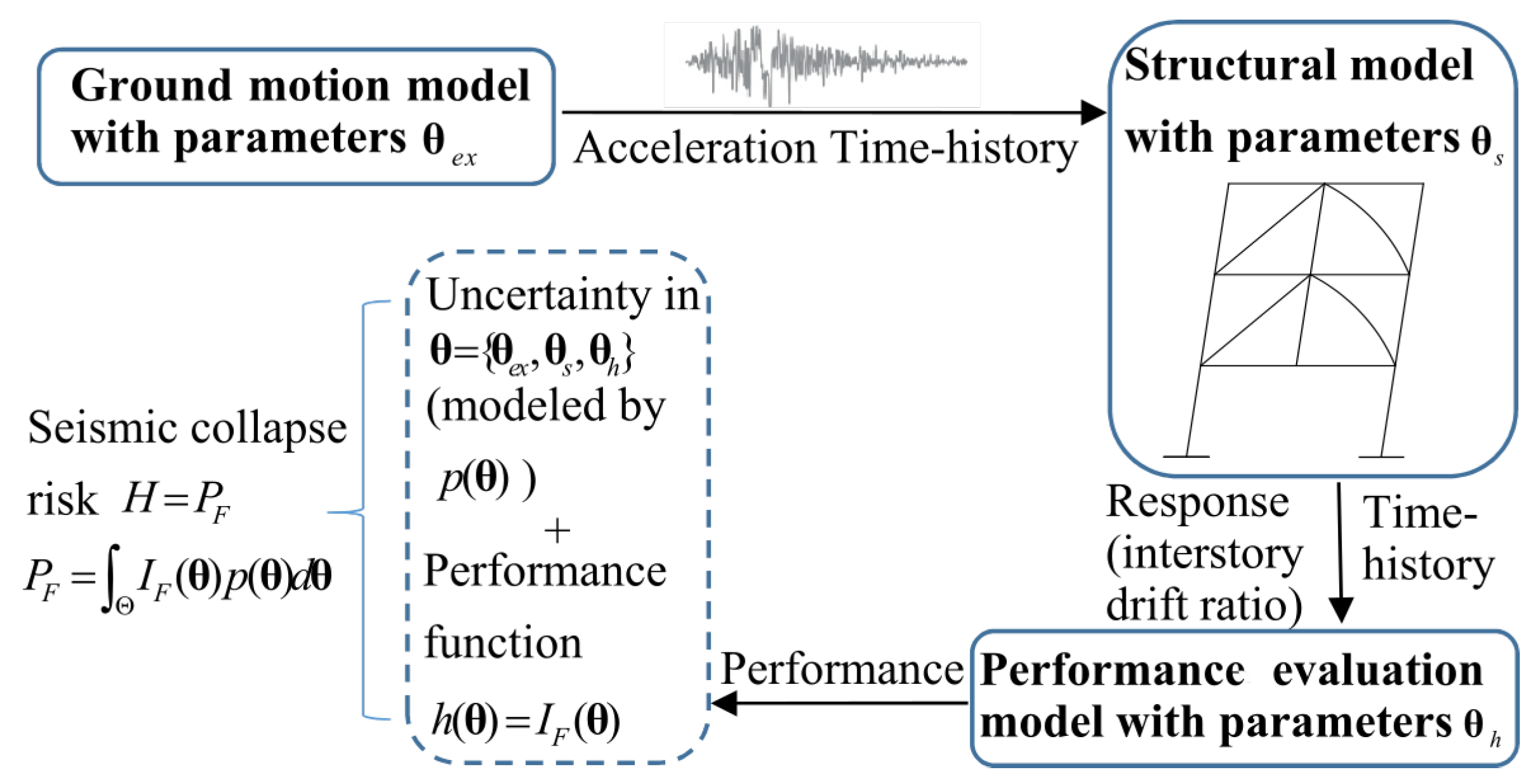
2.1. Simulation-Based Framework for Seismic Collapse Risk Quantification

To quantify the seismic collapse risk of braced frames, the simulation-based framework proposed in [16] for seismic risk assessment of base-isolated structures was adopted, since it can explicitly quantify the uncertainties in the ground motions and allows adoption of complex probability models and structure models. In the current study, the focus was on assessing the seismic collapse risk of braced frames. The framework in the context of seismic collapse risk quantification is shown in Figure 1. The framework is briefly reviewed here.
The framework defines an augmented system model that includes models for the excitation, the structure, and the probabilistic performance. Let θ Θ R n θ represent the augmented n θ -dimensional vector of uncertain model parameters, where Θ corresponds to the entire domain for all the possible values for the uncertain parameters. θ is composed of model parameters for the excitation (denoted θ e x ), the structural system (denoted θ s ), and the performance ( θ h ). For given specific θ , the risk consequence measure is denoted h ( θ ) , which can be evaluated based on the corresponding structural response (denoted y ( θ ) ). To address the uncertainty in θ , proper PDFs can be assigned, which is denoted p ( θ ) . The seismic risk H can be quantified as the expected value of h ( θ ) over the probability models for θ , H = E θ [ h ( θ ) ] = Θ h ( θ ) p ( θ ) d θ . Based on the different definition for h ( θ ) , different seismic risk H can be established. In this study, we are interested in the seismic collapse risk or the probability of collapse. As such, h ( θ ) = I F ( θ ) , where I F ( θ ) is the indicator function for the failure event F (i.e., structural collapse) and takes value of 1 if F occurs and 0 otherwise. The seismic collapse probability or risk P F can be written as
P F = Θ I F ( θ ) p ( θ ) d θ

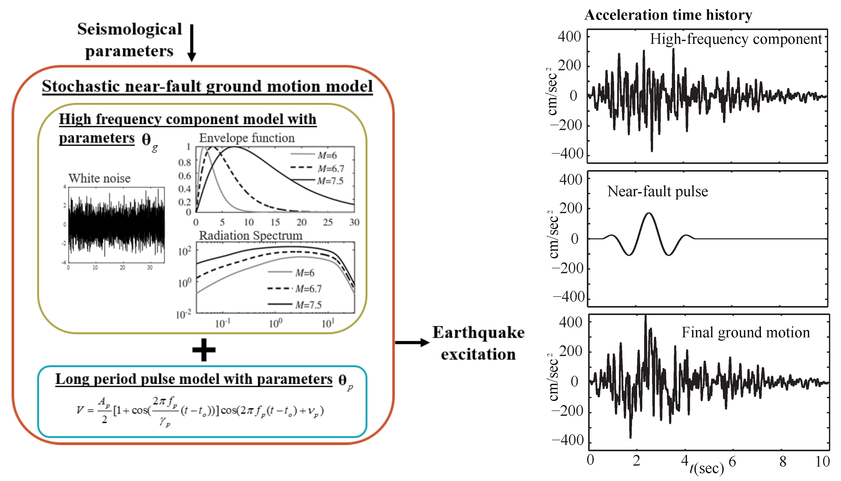
2.2. Stochastic Near-Fault Ground Motion Model

To assess the seismic collapse risk under near-fault earthquakes, the uncertainty associated with the seismic hazard (including the near-fault characteristics) needs to be properly quantified. Considering the scarcity in recorded near-fault ground motions, a stochastic near-fault ground motion (SGM) model was used to generate synthetic ground motions, instead of using real scaled ground motions. In this study, the probabilistic excitation model described in [19] was adopted. The near-fault stochastic ground motion (i.e., the acceleration time history) is established by modeling the high-frequency component and the near-fault characteristics independently and then combining them to form the final acceleration time history [24] where the near-fault pulse characteristics are explicitly incorporated in the SGM model. Figure 2 illustrates the SGM and shows a sample ground motion acceleration time history generated by the SGM.
By assigning appropriate PDFs to the model parameters, the uncertainty in the seismic hazard can be conveniently addressed. In addition, since not all near-fault excitations will have a velocity pulse, the probability of pulse occurrence needs to be integrated into the stochastic model as well. This is established by introducing a discrete random variable ε p with outcomes as either yes or no (also referred as the pulse existence parameter). The probability of having pulse (i.e., probability of ε p = y e s ) is estimated as a function related to the seismicity characteristics [25]. Overall, the uncertain model parameters include seismological parameters such as moment magnitude M, rupture distance r, parameters related to the high frequency components θ g , and the pulse parameters θ p , and white noise sequence Z w . For completeness, the high-frequency component model and near-fault pulse model including their model parameters and distributions are described in Appendix A.

3. Seismic Collapse Risk Assessment and Sensitivity Analysis Using Efficient Simulation

This section discusses the efficient simulation-based approach for evaluation of the seismic collapse risk integral and sample-based approach for probabilistic sensitivity analysis to identify the relative importance of different uncertain model parameters in the stochastic ground motion model towards seismic collapse risk. The overall process is illustrated in Figure 3.

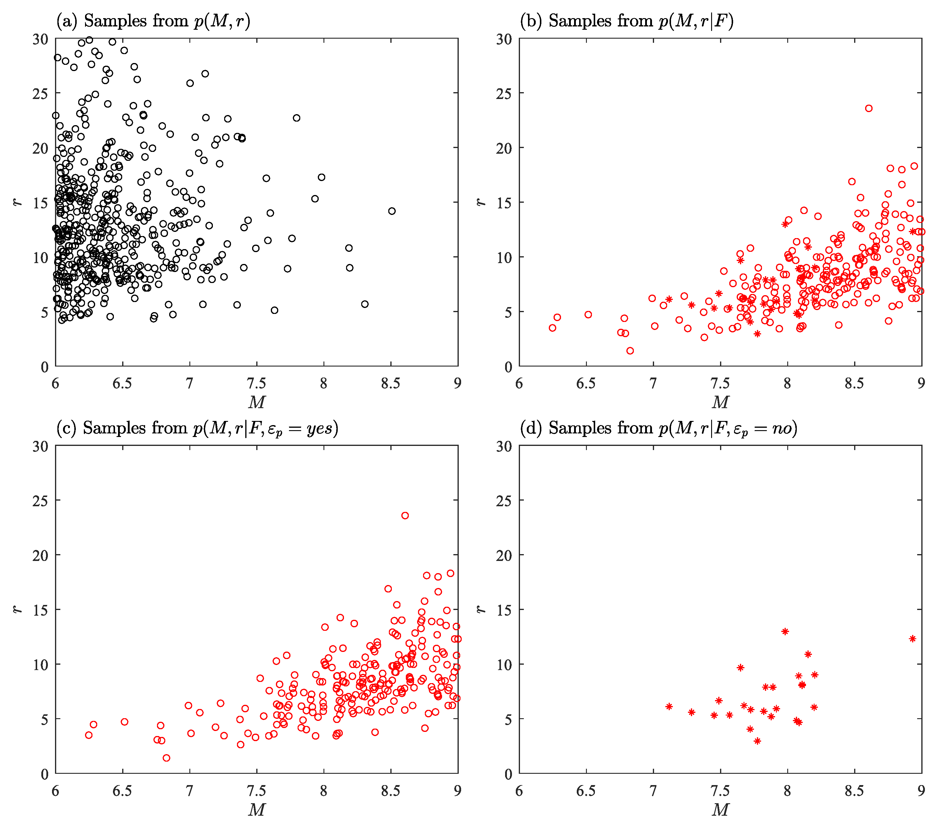
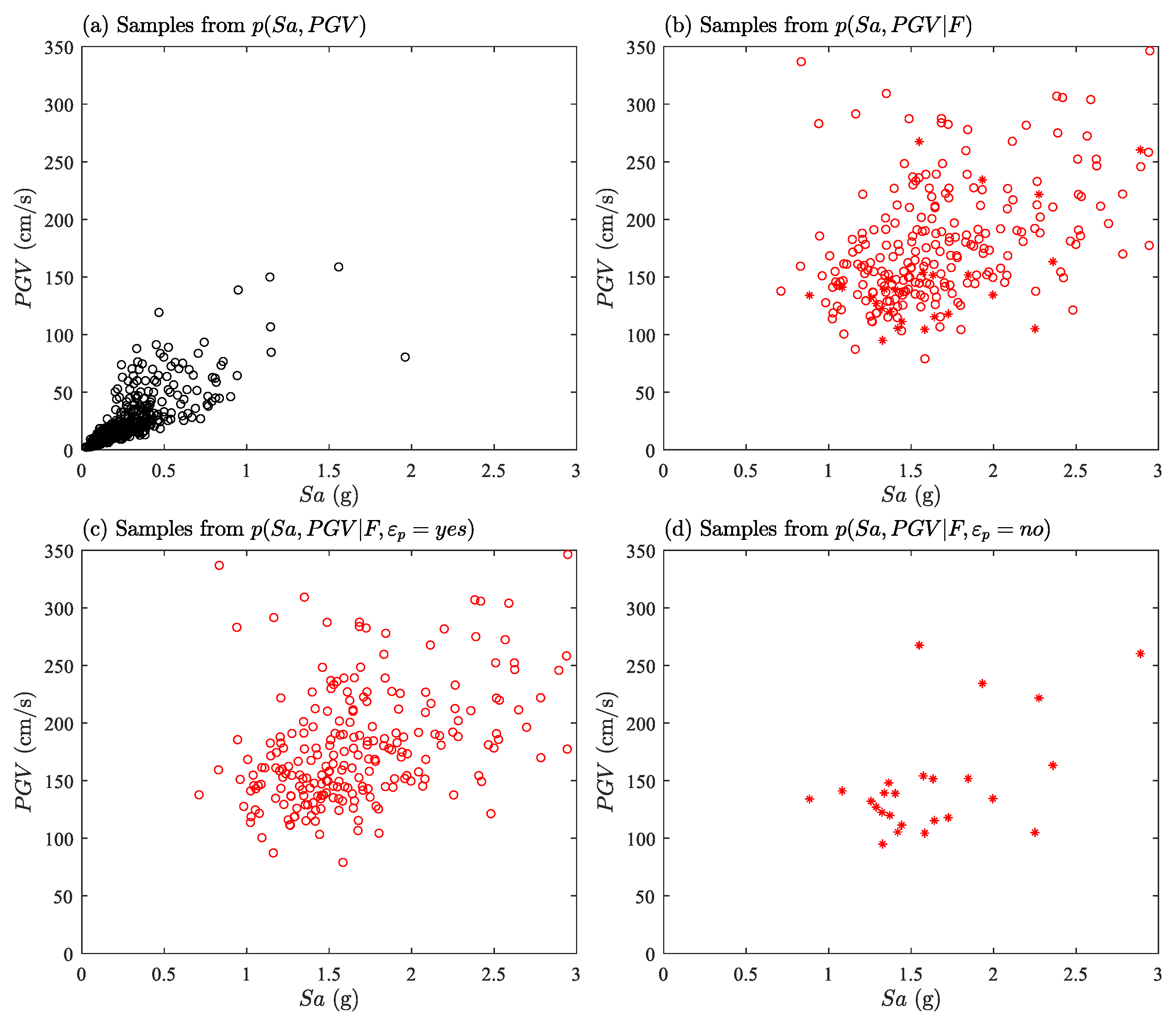
3.1. Stochastic Simulation for Seismic Collapse Risk Assessment

To evaluate the risk integral, stochastic simulation can be used, since it is general and can address complex models and high-dimensional uncertainties. More specifically, using N samples from some proposal density q ( θ ) , an estimate for P F is established by
P ^ F = 1 N j = 1 N I F ( θ j ) p ( θ j ) q ( θ j )
where θ j represents the sample in the j t h simulation. The accuracy of the estimation can be evaluated through its coefficient of variation (c.o.v) δ [26]. Lower values of δ means better accuracy. To improve the accuracy and efficiency of the estimation, importance sampling can be adopted, which corresponds to choosing a better proposal density (i.e., importance sampling density) q ( θ ) by focusing on regions of the Θ space that contribute more to the integrand of the risk integral.
For problems with high-dimensional uncertainty, importance sampling density q ( θ ) can be established focusing on the important dimensions/parameters that have more impact than the others towards the integrand. For the current problem, it is expected that ground motion model parameters such as moment magnitude, rupture distance, and amplitude of pulse may have large impacts on the seismic collapse risk, and proposal density will be built with respect to those parameters to improve the estimation accuracy and efficiency. When the failure probability is small, besides importance sampling, other advanced stochastic simulation techniques can also be used [27,28,29].

3.2. Efficient Estimation of Conditional Seismic Collapse Risk

To estimate the seismic collapse risk of the braced frame under stochastic near-fault ground motions (i.e., with probabilistic pulse), Equation (2) is used. For comparison purposes, the seismic collapse risk under stochastic ground motions without near-fault pulse is also calculated to assess the amount of increase of collapse risk due to near-fault pulses. To evaluate the seismic collapse risk when the near-fault pulse is neglected, instead of performing additional simulations (i.e., under stochastic ground motions without the near-fault pulse), which are computationally expensive, an efficient approach using the Bayes’ theorem is developed to directly calculate the corresponding seismic collapse risk using the same set of N simulations (i.e., without running additional simulations).
More specifically, the failure probability of the structure when there is no near-fault pulse in the ground motion, P ( F | ε p = n o ) , can be written as follows using the Bayes’ theorem
P ( F | ε p = n o ) = P ( ε p = n o | F ) P F P ( ε p = n o )
Based on the existing simulations, using Equation (2), we can establish an estimate P ^ F for P F , which corresponds to the seismic collapse risk. P ( ε p = n o ) corresponds to the marginal probability of no pulse in the ground motion under the prior distribution p ( θ ) , and is equal to 1 P ( ε p = y e s ) where P ( ε p = y e s ) corresponds to the marginal probability of having pulse under the prior distribution and has the expression P ( ε p = y e s ) = P ( ε p = y e s | θ r ) p ( θ r ) d θ r , where θ r corresponds to the rest of the parameters excluding ε p . Using the existing N simulations, P ( ε p = y e s ) can be estimated through
P ^ ( ε p = y e s ) = 1 N j = 1 N P ( ε p = y e s | θ r j ) p ( θ r j ) q ( θ r j )
Therefore, P ( ε p = n o ) can be estimated as P ^ ( ε p = n o ) = 1 P ^ ( ε p = y e s ) .
As to P ( ε p = n o | F ) , it can be estimated from the failure samples from the so-called failure distribution p ( θ | F ) , which is proportional to the integrand of the seismic collapse risk integral and has the expression p ( θ | F ) = I F ( θ ) p ( θ ) / P F I F ( θ ) p ( θ ) . In particular, using the existing simulations, a stochastic sampling algorithm (e.g., rejection sampling) can be used to generate samples from the failure distribution (as illustrated in Figure 3), giving total of N F failure samples. Then, P ( ε p = n o | F ) can be estimated by P ^ ( ε p = n o | F ) = N F , ε p = n o / N F where N F , ε p = n o corresponds to the number of failure samples that do not have near-fault pulse. Note that these failure samples will be used later for efficient probabilistic sensitivity analysis as well.
Therefore, in the end, an estimate for P ( F | ε p = n o ) can be established as
P ^ ( F | ε p = n o ) = P ^ ( ε p = n o | F ) P ^ F P ^ ( ε p = n o )

3.3. Probabilistic Sensitivity Analysis Using Sample-Based Approach

To identify the uncertain model parameters in the ground motion model (including the pulse characteristics) that have a higher contribution towards the seismic collapse risk of braced frames, we use the probabilistic sensitivity measure called relative entropy proposed in [16]. The foundation of this sensitivity analysis is the definition of an auxiliary PDF p ( θ | F ) proportional to the integrand of the seismic collapse risk integral, which in the current problem corresponds to the failure distribution for θ mentioned earlier. Comparison between the marginal distribution p ( θ i | F ) and the prior distribution p ( θ i ) indicates the sensitivity with respect to the uncertain parameter θ i . The difference between these two PDFs is quantified by relative entropy
D p ( θ i | F ) | | p ( θ i ) = Θ i p ( θ i | F ) log p ( θ i | F ) p ( θ i ) d θ i
A larger relative entropy value indicates greater importance in affecting the seismic collapse risk. This idea is not limited to a particular single parameter θ i and can be extended towards a set of uncertain parameters (e.g., group of parameters { θ i , θ j } ) by comparing the corresponding marginal distributions for these parameters.
To efficiently estimate the relative entropy for each individual parameter and also groups of parameters, which requires the estimation of the corresponding marginal auxiliary distribution (corresponding to multidimensional integral), the sample-based approach in [16] is used. It relies on generating samples from the joint failure distribution p ( θ | F ) , also called failure samples. Then, the projection of these samples to spaces representing each uncertain parameter gives samples from the corresponding marginal failure distribution p ( θ i | F ) . Then, based on the marginal samples, an estimate of the marginal PDF can be established using kernel density estimation (KDE) [16,30]. More details about the sample-based approach can be found in [16,31].
In the context of seismic collapse risk estimation, instead of conducting additional simulations to generate the failure samples, we use the readily available information in the N simulations for estimating the seismic collapse risk and directly apply rejection sampling to these samples to generate the failure samples; therefore, the probabilistic sensitivity analysis is carried out efficiently with no additional simulations (as illustrated in Figure 3). In addition to continuous variables, relative entropy can also be defined for discrete variables, where the integration becomes summation over all the values that the discrete variable can take, and the PDFs correspond to probability mass functions (PMFs). In the current problem, to explicitly investigate the sensitivity of the seismic collapse risk with respect to the existence of near-fault pulses, we investigate the sensitivity with respect to the discrete pulse existence parameter ε p . The relative entropy for ε p is calculated through
D P ( ε p | F ) | | P ( ε p ) = P ( ε p = y e s | F ) log P ( ε p = y e s | F ) P ( ε p = y e s ) + P ( ε p = n o | F ) log P ( ε p = n o | F ) P ( ε p = n o )
where P ( ε p = y e s | F ) can be estimated by P ( ε p = y e s | F ) = N F , ε p = y e s / N F where N F , ε p = y e s is the number of failure samples with pulse and N F is total number of failure samples generated. P ( ε p = y e s ) can be estimated using Equation (4) as described earlier. In the end, the relative entropy for ε p can be established. The relative importance of ε p can be compared with other model parameters by comparing their relative entropy values.

4. Illustrative Example

This section describes the two braced frames that will be studied as an illustration. The focus is on assessing and comparing their seismic collapse risk, and identifying the impact of near-fault earthquakes and associated uncertainties on the seismic collapse risk of the braced frames.

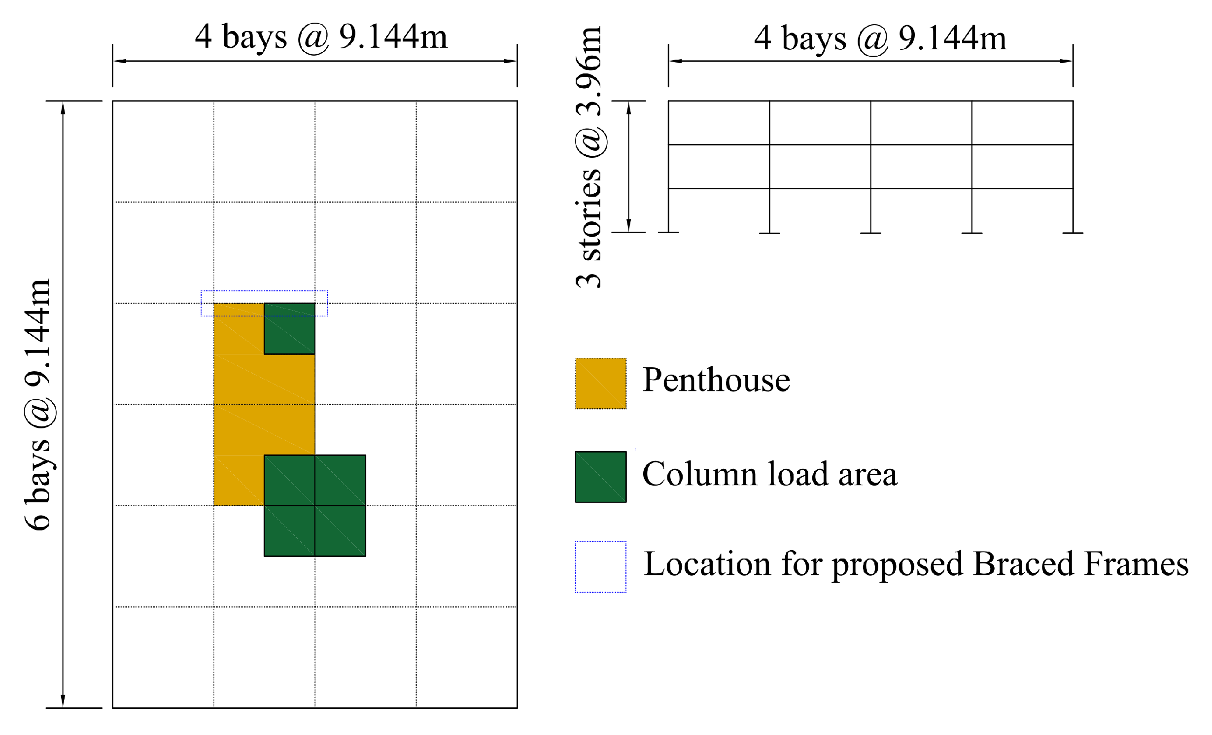
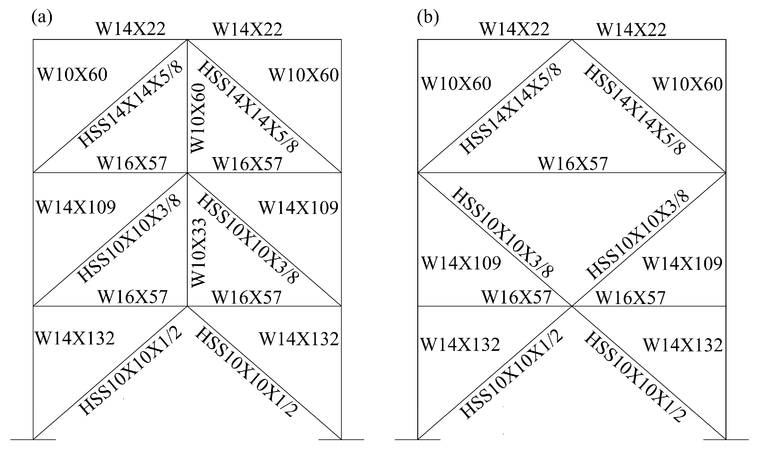
4.1. The Example Braced Frames

In this study, the building from the SAC Joint Venture project (which is a moment-resisting frame) was used. The model building was designed based on local code requirements for three different cities (i.e., Los Angeles, Seattle, and Boston) [32]. For this study, the three-story model building was redesigned as an office building and modeled as a braced frame. The floor plan and elevation view of the three-story SAC building are illustrated in Figure 4. Moment resisting frames are utilized in the periphery of the office building. In the current study, the braced frames are designed at the perimeter of the penthouse located at the two bays in each direction of the building. Two configurations of the braced frame in [33] are considered: chevron bracing with zipper columns and cross-bracing system (shown in Figure 5).
All the loads (dead and live load) acting on the different floor and their distribution are obtained from Appendix B in FEMA 355C [32]. The self-weight of the steel here is assumed to be 0.622 kN/m 2 [32]. The given loading definition is used to estimate the seismic mass of the structure, which has values of 10,155 kN, 9386 kN, and 9386 kN for the mass of roof, third floor, and second floor, respectively. The FEMA guidelines are used to calculate the lateral load acting on this system. The structure modeled here is assumed to be located in Los Angeles with site class C.
After the quantification of the load acting on the structure including both lateral and gravity loads, a load-resisting system was selected to maintain the overall stability and integrity of the structure under high seismic events. As mentioned earlier, the lateral load-resisting systems selected in this research are braced frames with chevron bracing and cross bracing. Next, the design and some details of these systems are presented. For both braced frames, the structural steel was assumed to be Grade 50 A 992 with a modulus of elasticity E = 200 GPa and yield strength f y = 345 MPa.
The chevron-braced frames are one of the types of SCBFs in which proper detailing and design can lead to a high-performance system with good ductility and energy dissipation proficiency [34]; however, these systems can exhibit typical braced frame problems under high seismicity. Under large lateral displacements, the brace in compression may buckle prematurely and its axial load carrying capacity is decreased tremendously while the tension in the other braces continues to increase. This mechanism creates unbalanced vertical forces on the beam, and thus the overall lateral strength of the system is reduced. In order to counteract this effect, the zipper columns can be added at the intersection of the beam and the braces [35]. Here, zipper columns with partial height zipper mechanisms were adopted as it results in better distribution of the loads and energy over the height of the structure, thus maintaining the stability of the structure. In order to ensure that the system behaves in the intended manner, the two-phase design procedure proposed in [36,37] was used. In the first phase, the frame member sizes are determined to resist the lateral and the gravity loads calculated in the previous section. This corresponds to the strength design of the system without the utilization of the zipper column [36]. Hollow steel section (HSS) members are used for braces. The second phase involves the capacity design of the system in which the zipper columns are introduced to resist the vertical unbalanced force generated by the brace at each individual levels. The top story braces are designed to elastically resist the vertical unbalanced forces collected by the zipper columns below the top story and the top-floor equivalent earthquake force [33,37]. The design methodology of the cross-braced system is relatively straightforward. This system was designed by first deciding the configuration of the braces in the lateral load-resisting system and then subjecting it to lateral loads. Figure 5 shows the sections used for both frames.

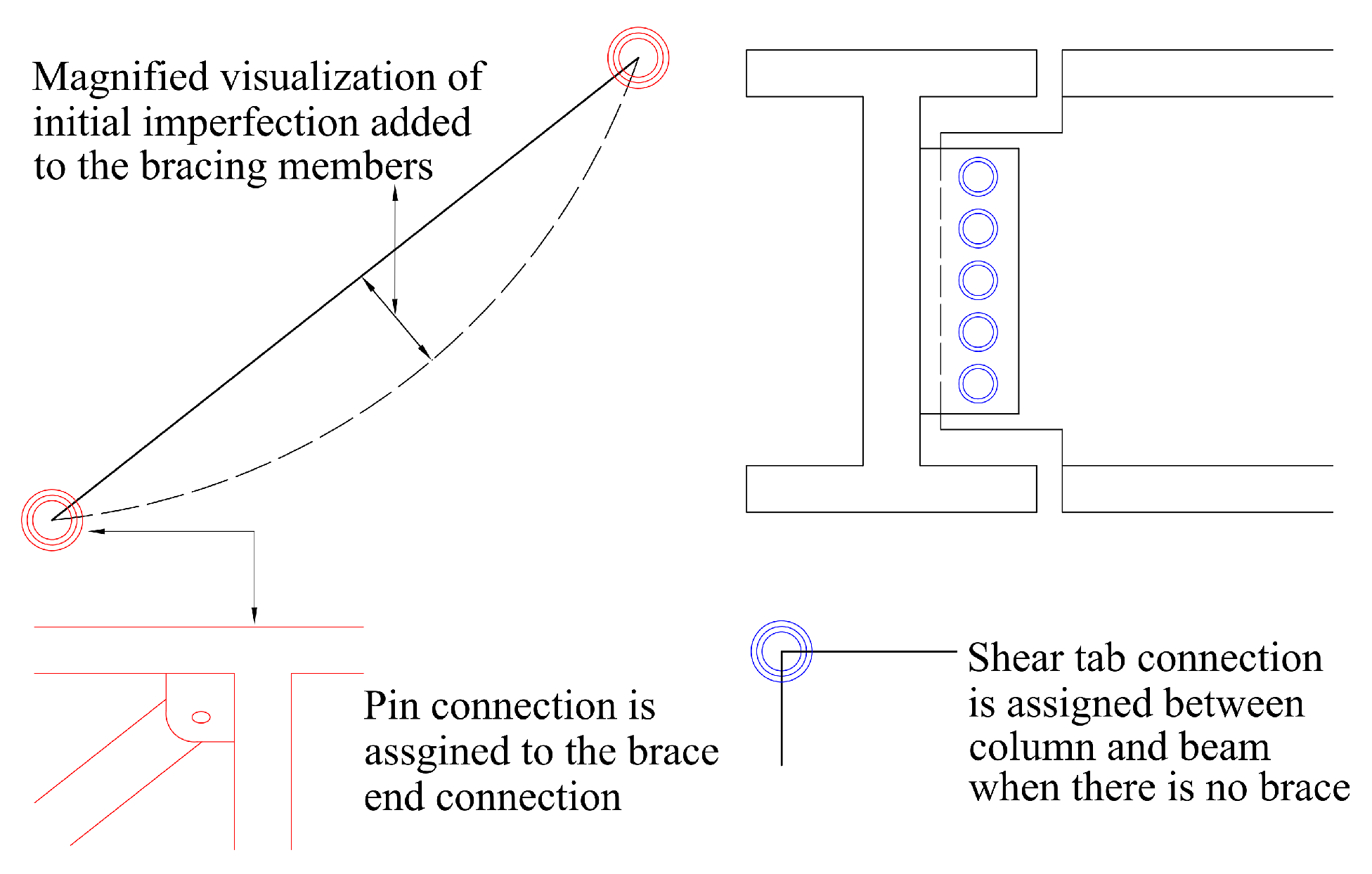
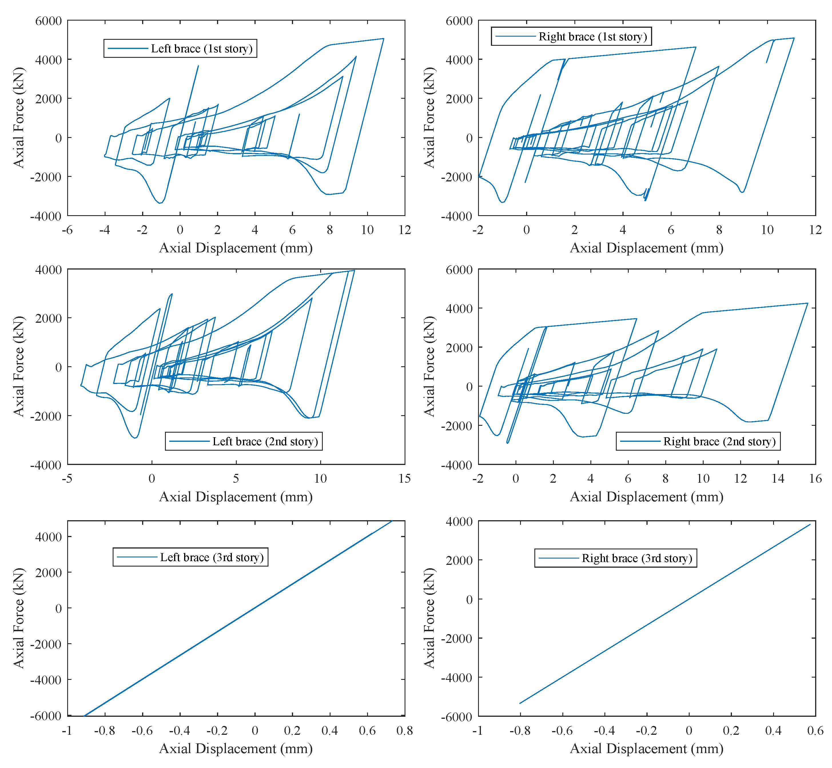
4.2. Numerical Modeling of the Example Braced Frames

For numerical modeling and analysis of the braced frames, ZEUS-NL, which is an open source software, was used [38]. ZEUS-NL can handle large inelastic displacement analysis for complex frames using the fiber approach and it has a suite of commonly used material models and elements. The beams, columns, and the braced elements are modeled as fiber sections. A bilinear elasto-plastic model with kinematic strain hardening material was utilized for the elements where a strain hardening factor μ = 0.03 is used. The end condition of the braced frames is taken as ‘pin-connection’ (see Figure 6), which is modeled by using a zero-length spring element at the brace’s ends with almost zero initial stiffness. In addition, the initial imperfections in the braces (shown in Figure 6) are assumed to be in-plane with a value of 0.1% of the effective length of the braces [39]. A shear tab connection is also assigned between columns and beams when there is no brace connected to them (see Figure 6). A rotational spring is used to model the shear tab connection at the top story beam for both frames and also on the first floor for the cross-braced frame. The damping is modeled using Rayleigh damping with a damping ratio of 5% corresponding to the fundamental frequency. To validate the above modeling approach, an example braced frame from OpenSees was analyzed, and the results (from pushover analysis, dynamic analysis, and eigenvalue analysis) are compared against published results obtained from the analysis by OpenSees [40]. Then, the above modeling approach was used to build numerical models for the two example braced frames. To obtain the dynamic properties and behavior/performance of the braced frames, eigenvalue analysis and pushover analysis were carried out using the developed numerical models. The chevron-braced frame has a period of 0.708 s while the cross-braced frame has a slightly longer period of 0.720 s. The pushover curves for the braced frames are shown in Figure 7.
Previous research has shown that the braces in SCBFs are susceptible to low-cycle fatigue and fatigue induced fracture under strong earthquakes. To accurately capture the impact of the local brace behavior on the global seismic performance of the SCBFs, different models have been proposed in the literature [39,41,42,43,44,45,46,47]. For example, in OpenSees, a modified rainflow cycle counting algorithm is used to accumulate fatigue damage in a material, based on Coffin–Manson criterion, using Miner’s rule. Element stress/strain relationships become zero when fatigue life is exhausted. This model has been used to capture the low-cycle fatigue of braces in SCBFs. Further, Hsiao et al. [43] proposed a fracture modeling approach that simulated the nonlinear, cyclic response of SCBFs by correlating onset of fracture to the maximum strain range in the brace (i.e., the total distance between the maximum positive and maximum negative strain). The model accounts for important brace design parameters including slenderness, compactness, and yield strength; fracture data from over 40 tests were used to calibrate the model. In this paper, we use the maximum strain range formula developed in [43] to determine whether low-cycle fatigue rupture occurred or not, i.e., if the maximum strain range exceeds the limit given by the formula then fatigue rupture occurs. To do this, we keep track of the strain time history of all the braces in the frame during the time history analysis and use this information to calculate the maximum strain range under given ground motion. Although specific low-cycle fatigue fracture model is used in this study, the flexibility of the seismic collapse risk assessment framework can allow other models to be directly incorporated in the framework as needed.
To conduct initial assessment of the performance of the braced frames under cyclic load due to earthquakes, we first run the dynamic time history analysis for both frames under a selected ground motion. Here, the ground motion in [40] was used. Figure 8 shows the force deformation relationship at the middle of the braces in different stories in the chevron-braced frame. One important observation is that the third-story braces behave elastically as intended by design. As mentioned earlier, the top-story braces are designed to elastically resist the vertical unbalanced forces collected by the zipper columns below the top story and the top-floor equivalent earthquake force [33,37]. Figure 9 shows the hysteretic behavior of the chevron-braced frame including the story shear vs. interstory drift ratio (in %) for each story. Overall, the second story has the largest story drift, while the top story has the smallest story drift and is much smaller than the other two stories. This behavior (i.e., the third story has the smallest drift) is expected since the braces remain elastic, and the frame is designed to behave in such a manner. Figure 10 and Figure 11 show the respective behaviors for the cross-braced frame. For this frame, the braces at all stories undergo inelastic deformations. The top-story drift is much larger than that of the chevron-braced frame, and it is also the largest among all the stories with the second story having the smallest drift.

4.3. Implementation Details of the Simulation-Based Assessment of Seismic Collapse Risk

To evaluate the seismic collapse risk, the stochastic simulation-based approach for risk estimation described earlier was used. The simulation-based approach requires N evaluations of the structural response under simulated ground motions, which corresponds to nonlinear time history analysis and is the most computationally expensive task in the overall seismic risk assessment. For each simulation, the maximum interstory drift ratio of the braced frame was calculated and the maximum strain range was also calculated for all the braces in the frame based on the strain time history. In terms of the definition of structural collapse (i.e., failure), besides the interstory drift ratio, we also consider the low-cycle fatigue failure of braces, i.e., we assume that collapse occurs when either the maximum interstory drift ratio exceeds the collapse threshold (taken as 5% here) or the any of the braces fails due to low-cycle fatigue rupture. Note that the occurrence of collapse may depend on many factors and the collapse threshold typically also has variability, which can be considered by introducing uncertainty in this threshold (i.e., another parameter in θ ). Here, since the focus is on uncertainty in the ground motion, a deterministic collapse threshold was used. Then, using results from all the simulations, the seismic collapse risk was calculated using Equation (2) for both braced frames. Subsequently, information from this set of simulations was used within rejection sampling algorithm to generate samples from the failure distribution p ( θ | F ) . These failure samples are then used within a sample-based approach to efficiently evaluate the relative entropy for sensitivity analysis. The relative entropy values are used to identify the relative importance of different uncertain model parameters in the stochastic ground motion model towards seismic collapse risk.
For the case studies, the prior distributions for the above uncertain model parameters are as follow. The uncertainty in the moment magnitude for seismic events, M is modeled by Gutenberg–Richter relationship truncated in M m i n , M m a x = 6 ,   9 which leads to the following PDF
p ( M ) = b M exp ( b M M ) exp ( b M M min ) exp ( b M M max )
where b M = 0.9 ln 10 . The rupture distance r is assumed to follow a lognormal distribution with a median of r m e d = 12 km and c.o.v of r c o v = 45 % . The error for the amplitude of pulse A p , e A p , follows normal distribution with mean μ e A p = 0 and standard deviation σ e A p = 0.187 . Here, M and r are assumed to be independent for modeling convenience, with the understanding that for specific source geometries the rupture distance may not be independent of the moment magnitude. For example, a large magnitude event would most likely entail larger rupture area, so proximity of the site to the fault may not be independent of magnitude. These distribution models are selected and modified based on [19] to illustrate the proposed framework. While such selection affects the exact results for the illustrative example, it does not affect the validity of the proposed risk assessment framework. Since the framework is general, it can easily accommodate different probability distribution models, and when detailed information regarding the site-specific fault geometry and the joint distribution of moment magnitude and rupture distance is available for the interested site, it can be directly incorporated in the risk assessment framework.
To carry out the stochastic simulation, we need to have some proposal density q ( θ ) to generate realizations for the model parameters θ . The selection of this proposal density will affect the overall efficiency and accuracy of the seismic collapse risk estimation and the efficiency of the rejection sampling algorithm. Since typically collapse corresponds to rare events, if we directly use the prior distribution p ( θ ) as proposal density, we would need many simulations to generate realizations that will lead to collapse. From the view of importance sampling, we need to have a proposal density that can simulate more samples that lead to collapse. Intuitively, large earthquakes or earthquakes with strong intensity will tend to lead to structural collapse. It makes sense to select a proposal density that generates more samples with large earthquakes. To this end, proposal densities are prescribed for M (moment magnitude), r (rupture distance), and A p (amplitude of pulse) with the idea that q ( θ ) should be selected so that there are more samples for large M, small r, and large A p .
The following proposal densities are used for the above uncertain parameters. q ( M ) is selected as a truncated Gaussian distribution between 6 , 9 with a mean of 8.5 and standard deviation of 1. The proposal density for r is selected as lognormal distribution with median r m e d = 6 km (i.e., smaller rupture distance) and c.o.v of r c o v = 45 % . The proposal density for the amplitude of pulse characteristics depends upon the new proposal density for rupture distance and e A p ; the latter is selected as the normal distribution with the mean 0.15 and standard deviation of 0.187. For the rest of the parameters, the corresponding prior distributions are used. With the above selection of proposal density, N = 5000 samples are used for the stochastic simulation.

5. Results and Discussions

5.1. Seismic Collapse Risk Assessment Results

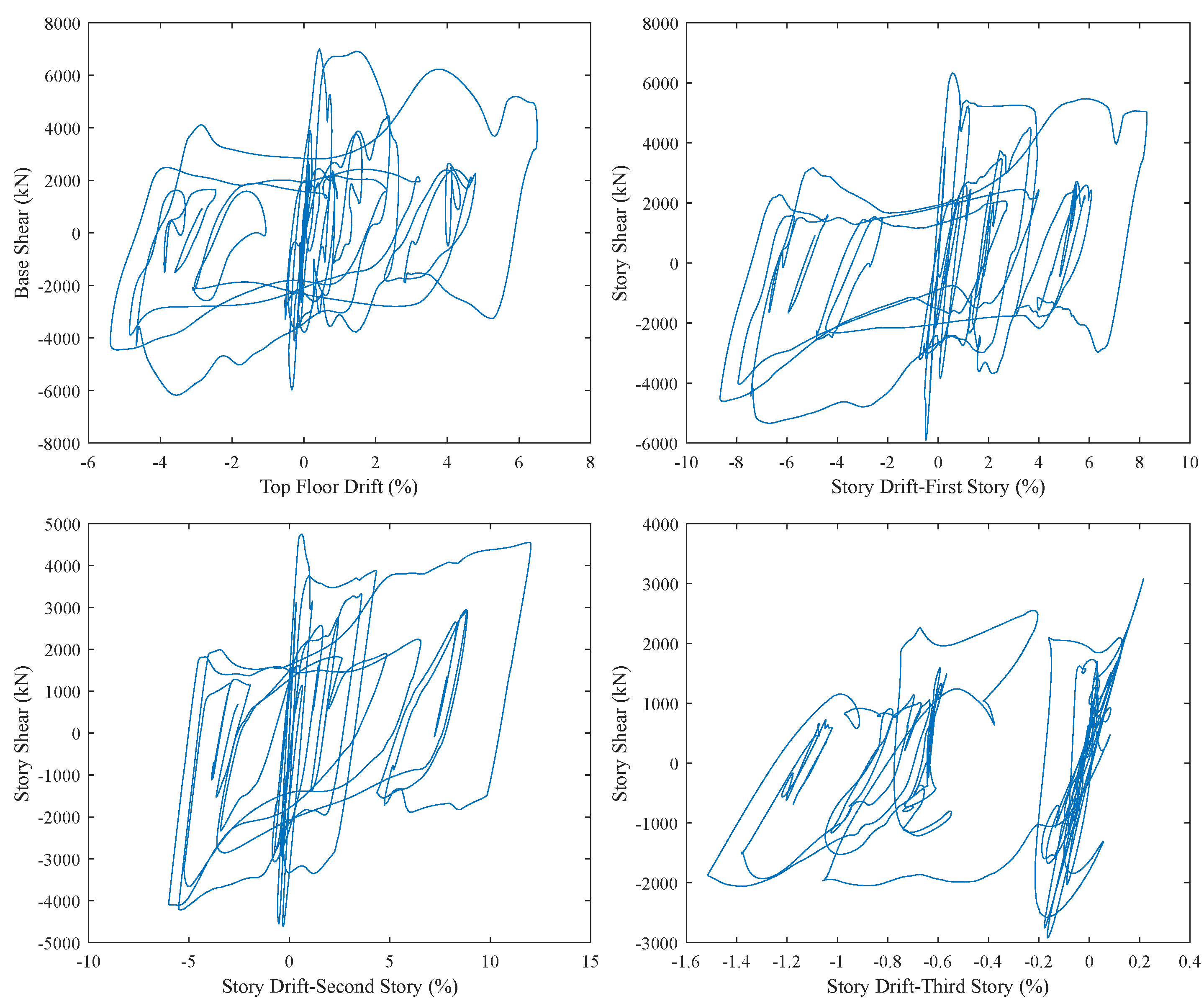
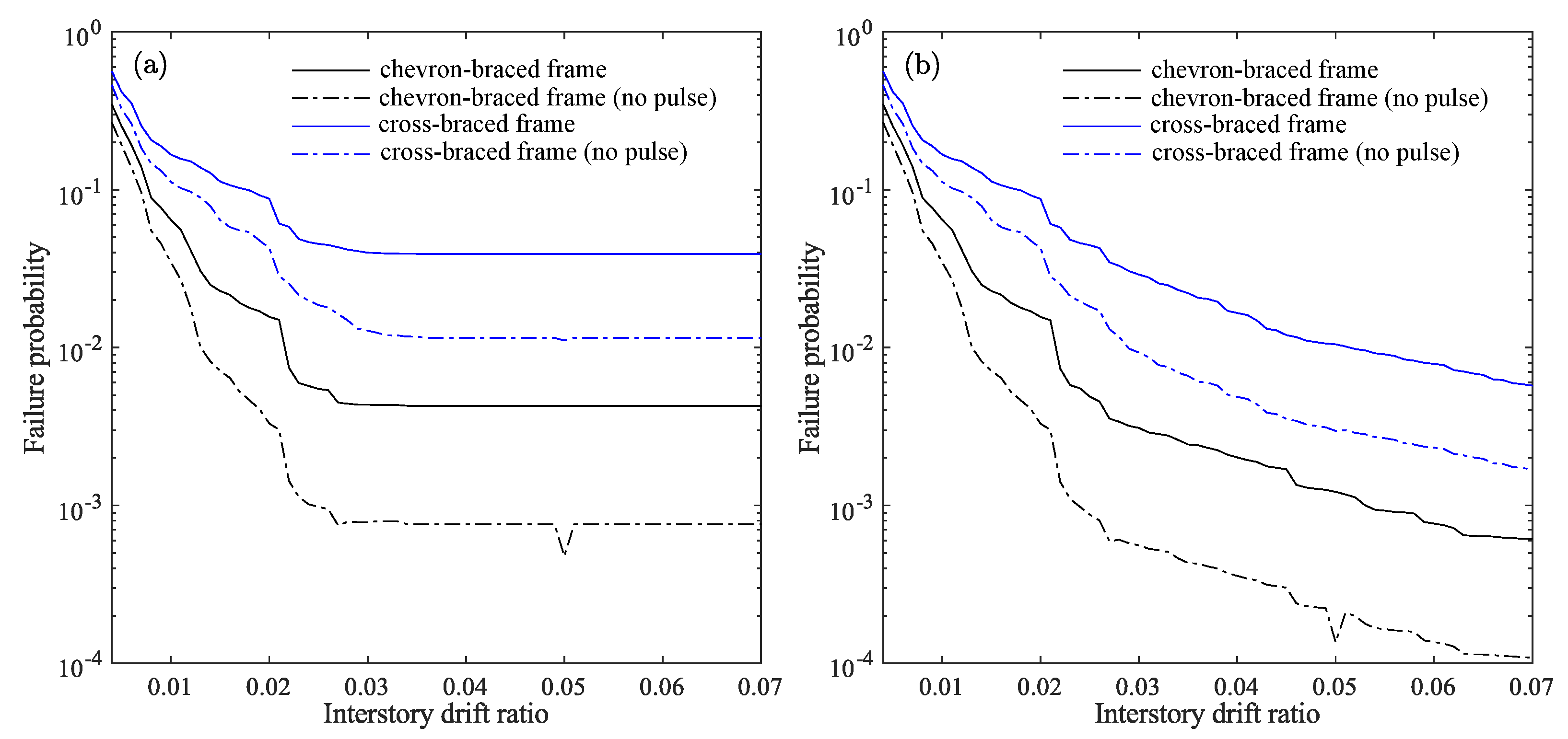
5.1.1. Chevron-Braced Frame

With the selected probability models, using Equation (2) with N = 5000 simulations, the seismic collapse risk of the chevron-braced frame is estimated to be P ^ F = 0.43%. To investigate the impact of including or not the near-fault pulse in the stochastic ground motion, the seismic collapse risk when there is no near-fault pulse in the stochastic ground motion is also evaluated. As mentioned earlier, this is performed using Equation (5) without running additional simulations. More specifically, P ( ε p = n o | F ) = N F , ε p = n o / N F is estimated to be 9.62%. Using Equation (4) (to calculate P ( ε p = y e s ) ) and P ( ε p = n o ) = 1 P ( ε p = y e s ) , P ( ε p = n o ) is estimated to be 86.28%. Plugging the values of P ( ε p = n o | F ) , P ^ F , and P ( ε p = n o ) into Equation (5) yields the failure probability P ( F | ε p = n o ) , which is estimated to be 0.05%. Compared to the seismic collapse risk of 0.05% when near-fault pulses are neglected, considering the probabilistic pulses leads to seismic collapse risk of 0.43%, which corresponds to an increase of almost 9 times the seismic collapse risk; therefore, for the current example, neglecting the near-fault pulse may lead to significantly underestimated seismic collapse risk.
Similar to calculation of P ( F | ε p = n o ) , P ( F | ε p = y e s ) , which corresponds to the seismic collapse risk when assuming all the ground motions have near-fault pulses, can be estimated as well. P ( F | ε p = y e s ) is estimated to be 2.82%, which further and more directly shows the impacts of near-fault pulses on the seismic collapse risk. From another perspective, under the prior distribution, the percentage of samples or ground motions that have near-fault pulse is P ( ε p = y e s ) = 13.72%. In comparison, for the failure distribution, in the samples or ground motions that caused failure, the percentage of ground motions that have near-fault pulse is P ( ε p = y e s | F ) = 90.38%, which corresponds to significant increase compared to P ( ε p = y e s ) . This further highlights that the occurrence of collapse failure in the considered chevron-braced frame is highly correlated to the existence of near-fault pulse. The results and comparisons here highlight the significant impacts of near-fault pulses on the seismic collapse risk estimation of the chevron-braced frame.
Besides the collapse failure probability, the variation of failure probability under different interstory drift ratio thresholds (i.e., the thresholds that define failure) is plotted in Figure 12 for both the case of considering probabilistic near-fault pulse and not considering near-fault pulse. To show the impact of low-cycle fatigue on the seismic collapse risk, the failure probability for the case when failure due to low-cycle fatigue is neglected is also shown in the figure (see Figure 12b). From Figure 12a, it can be observed that as the threshold increases the failure probability decreases first, which is expected, and then after certain drift ratio threshold (e.g., around 0.03 for chevron-braced frame), the failure probability does not decrease anymore and levels off. The latter is in contrast with the observation in Figure 12b, which shows that the failure probability will keep decreasing when the drift ratio threshold increases. The reason for this difference lies in the difference in the failure definition. In Figure 12a, beyond certain drift ratio threshold, the failure will be determined by the fatigue failure rather than the failure due to exceeding the drift ratio threshold, or in other words, the failure probability due to fatigue is always larger than the failure probability due to drift ratio exceedance. To further verify this, we also directly calculated the probability of failure due to only low-cycle fatigue, which is 0.43% and is the same value as the failure probability that the curve levels off at. Similar trend is observed for the case when the near-fault pulse is neglected. The above observations highlight the importance of incorporating low-cycle fatigue in the seismic collapse assessment of braced frames. The failure probabilities corresponding to different damage states are reported in Table 1 for both the case of considering probabilistic near-fault pulse and not considering near-fault pulse where the interstory drift ratio thresholds for ‘slight damage’, ‘moderate damage’, and ‘extensive damage’ are selected as 0.004, 0.008, and 0.025, respectively. As can be seen, for the case where there is no near-fault pulse in the ground motion, the corresponding failure probabilities for all the different levels of damage states are much smaller. This shows the importance of the near-fault pulse and how it can significantly increase the probability of failure in the structure. When the near-fault pulse is neglected, the corresponding seismic risk will be significantly underestimated; therefore, in general, for more accurate seismic risk assessment, it is important to accurately and properly characterize the near-fault pulses that might exist in near-fault ground motions.

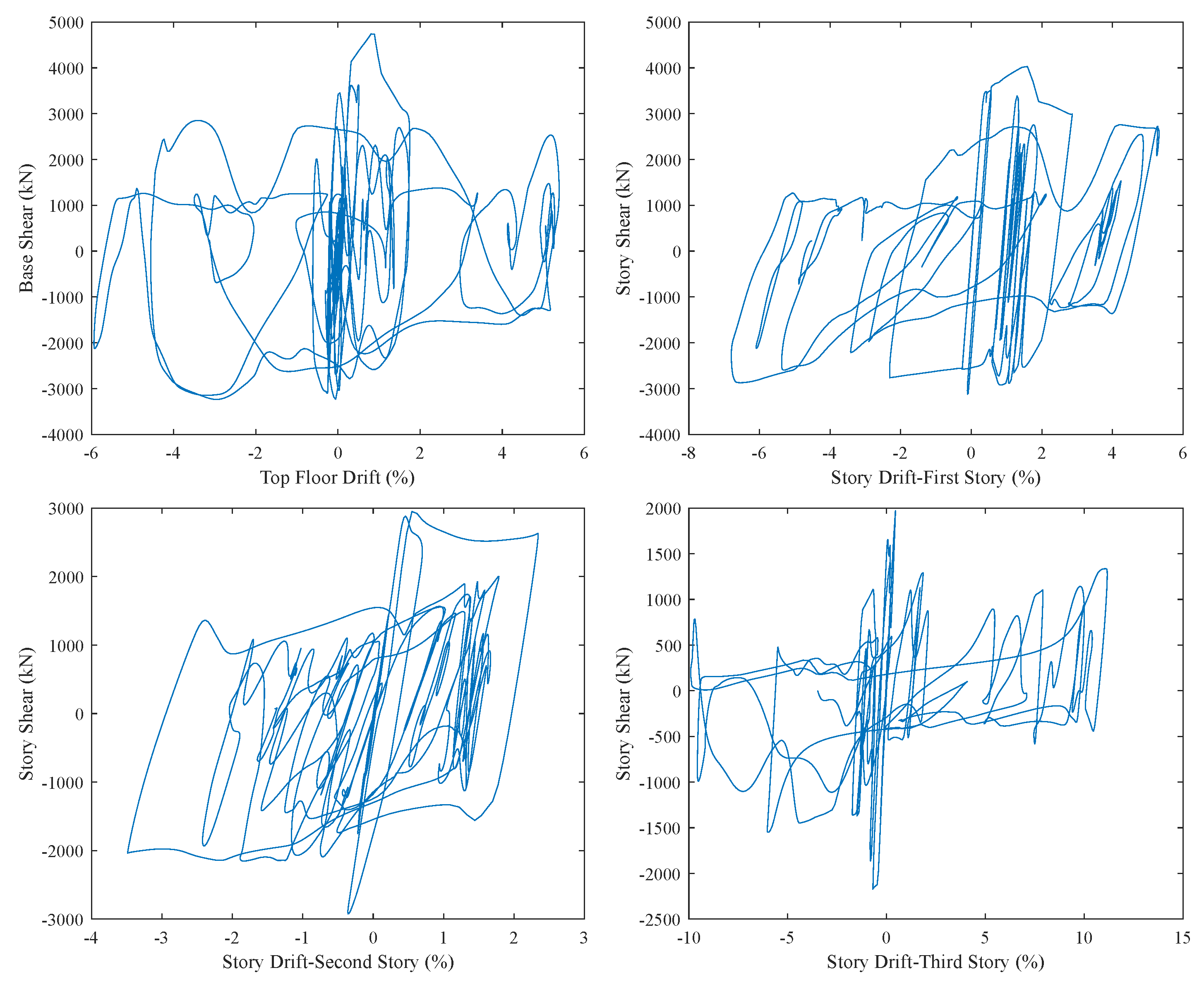
5.1.2. Cross-Braced Frame

Similarly, the failure probability P ^ F for the cross-braced frame is also calculated, which is estimated to be P ^ F = 3.92%. Using Equation (5), the failure probability P ( F | ε p = n o ) is estimated to be 1.11%. As can be seen, similar to the chevron-braced frame, considering near-fault pulse in the ground motions leads to increased seismic collapse risk for the cross-braced frame, highlighting the significant impacts of near-fault pulses on the seismic collapse risk estimation of the cross-braced frame. For cross-braced frame, P ( F | ε p = y e s ) is estimated to be 21.60%, which further and more directly shows the impacts of near-fault pulses on the seismic collapse risk. In the samples or ground motions that caused failure, the percentage of ground motions that have the near-fault pulse is P ( ε p = y e s | F ) = 75.62%, which also corresponds to a significant increase compared to P ( ε p = y e s ) = 13.72%, highlighting the strong correlation between the occurrence of collapse failure and the existence of a near-fault pulse. Overall, similar to the chevron-braced frame, the results show the importance of incorporating the near-fault pulses that might exist in near-fault ground motions for accurate estimation of the seismic collapse risk of cross-braced frames.
Besides the collapse failure probability, the variation of failure probability under different interstory drift ratio thresholds is also plotted in Figure 12 for both the case of considering probabilistic near-fault pulse and not considering near-fault pulse. The failure probabilities under different damage states are also reported in Table 1 for both the case of considering probabilistic near-fault pulse and not considering near-fault pulse. Similar trends to the chevron-braced frame are observed.

5.1.3. Comparison between the Two Braced Frames

Comparing the results for the two braced frames, it can be seen that the cross-braced frame has a much higher probability of failure for both the case of considering probabilistic near-fault pulse in the ground motions and the case of not considering near-fault pulse in the ground motions. The seismic collapse risk of the chevron-braced frame is around 0.43%, while the value for cross-braced frame is around 3.92%. The corresponding risks when not considering near-fault pulse are 0.05% and 1.11%, respectively. The higher seismic collapse risk for the cross-braced frame aligns with our observations in the earlier section when comparing the pushover analysis results for these two braced frames. For the pushover analysis, it was observed that after the braces buckle/yield for the cross-braced frame, it did not have any ultimate strength; therefore, the overall stiffness of the system decreased with the lateral displacement as opposed to the chevron-braced frame. This behavior conforms to the general braced frame behavior where braces act as the primary component for resisting the lateral forces due to seismic action. For the chevron-braced frame, the introduction of the zipper columns can also be enhancing the overall performance of the system. Based on earlier discussion on the behavior of the chevron-braced frame, the lower failure probability could also be attributed to the much smaller drift at the third story (as seen in Figure 9) and the fact that the third-story braces are designed to elastically resist the vertical unbalanced forces collected by the zipper columns below the top story and the top-floor equivalent earthquake force.

5.2. Probabilistic Sensitivity Analysis Results

In this section, probabilistic sensitivity analysis was carried out to quantify the importance of uncertain model parameters in the stochastic near-fault ground motion towards the seismic collapse risk. The calculation details for the relative entropy values for both continuous variables and discrete variables have been discussed in the earlier sections. Note that the same set of simulations were used to generate the failure samples from the failure distribution and no additional simulations were used to establish the relative entropy values for all the uncertain model parameters in the stochastic ground motion model. Additionally, the importance of the pulse existence parameter ε p is also calculated using Equation (7). The relative entropy results for some of the important parameters in the SGM that have a relatively large impact on the seismic collapse risk are presented for both frames.
Two general cases are considered. The first case corresponds to when there is probabilistic near-fault pulse in the stochastic ground motion (i.e., the existence of pulse has a certain probability, which is calculated based on Equation (A4)). This case is denoted as ε p = { y e s , n o } . The second case corresponds to when there is no near-fault pulse (i.e., only considering the high-frequency components in the stochastic ground motion). This case is denoted as ε p = { n o } . For the second case, essentially the model parameters in the stochastic ground motions will not have any of those parameters that are related to the pulse characteristics. The relative entropy for θ i in this case is calculated between p ( θ i | F , ε p = n o ) (instead of p ( θ i | F ) ) and the prior distribution p ( θ i ) , i.e.,
D p ( θ i | F , ε p = n o | | p ( θ i ) = Θ i p ( θ i | F , ε p = n o ) log p ( θ i | F , ε p = n o ) p ( θ i ) d θ i
where p ( θ i | F , ε p = n o ) is estimated (i.e., using KDE) based on the failure samples for θ i that do not have near-fault pulse. For both cases, only some of the important parameters for the corresponding case are presented. In addition to individual parameters, relative entropy is also evaluated for some groups of parameters to investigate the joint effects of these parameters. In terms of sensitivity analysis for resultant parameters, besides the ones discussed in Appendix A, the sensitivities for the two commonly used seismic intensity measures S a (corresponding to the first mode) and P G V are also calculated.

5.2.1. Chevron-Braced Frame

The relative entropy values for the chevron-braced frame are reported in Table 2. For the ε p = { y e s , n o } case, in terms of independent parameters, it is evident that the moment magnitude M dominates the risk with the rupture distance r having a much smaller influence. The group parameter [ M , r ] had the highest importance in seismic collapse risk. The higher importance of these parameters are expected since they are the primary seismological parameters that affect seismic risk. In terms of resultant parameters, S a has the highest importance, this is expected and consistent with research findings in the literature. Further, S a has been frequently used as the intensity measure to establish seismic collapse fragility considering the strong correlation between failure and the S a values. Similarly, high importance is observed for P G V as well, followed by the upper and lower frequencies of the high-frequency components in the ground motion f a and f b . Further, the pulse existence parameter ε p has high sensitivity values, demonstrating the importance of near-fault pulses on the seismic collapse risk. It can also be noted that the primary pulse characteristics (e.g., pulse period T p , pulse amplitude A p ) had a significant influence on the seismic collapse risk. The higher relative entropy values for T p is expected considering its direct dependence on the moment magnitude M (see Equation (A3)). Overall, the pulse characteristics are shown to be crucial in seismic collapse risk assessment, and these characteristics and associated uncertainties should be included when assessing the seismic collapse risk of structures situated close to earthquake faults. For the case ε p = { n o } , since there is no near-fault pulse, all parameters related to the pulse characteristics are not considered.
To facilitate a more in-depth understanding of the sensitivity analysis results, Figure 13 shows the samples for primary seismic hazard characteristics M and r from the joint PDF p ( M , r ) , the joint failure distribution p ( M , r | F ) , as well as from the conditional failure distributions p ( M , r | F , ε p = y e s ) , p ( M , r | F , ε p = n o ) . Looking at the samples from p ( M , r | F , ε p = y e s ) (i.e., the failure samples that have near-fault pulses), it can be observed that even with low seismic moment magnitude, the existence of pulse can lead to collapse in the structure if the distance between site and fault is low. This again confirms the importance of near-fault pulse for seismic collapse risk assessment, which should not be ignored when designing the structure close to fault regions. On the other hand, for p ( M , r | F , ε p = n o ) , the failure samples mainly concentrated in regions with relatively high moment magnitude M (but not quite high, e.g., below 8.5) and relatively small rupture distance. The reason that not many failure samples have larger than 8.5 moment magnitude may be because of the fact that based on Equation (A4) when r is small as M becomes larger, the probability of having near-fault pulse becomes larger, hence resulting in fewer samples without pulse.
Besides M and r, to relate the risk assessment results to the underlying seismic hazard, the respective samples for the commonly used seismic intensity measures S a (corresponding to the first mode) and P G V from the joint PDF p ( S a ,   P G V ) , the joint failure distribution p ( S a ,   P G V | F ) , as well as from the conditional failure distributions p ( S a ,   P G V | F , ε p = y e s ) , p ( S a ,   P G V | F , ε p = n o ) are also plotted and are shown in Figure 14. For the prior distribution, the S a and P G V concentrated in lower value regions, while for the failure samples from p ( S a ,   P G V | F ) , they correspond to much higher S a and P G V values. This is expected, since both intensity measures have been found to be correlated to the failure of structures and higher values of S a and P G V are more likely to cause failure of structures. When comparing the samples from p ( S a ,   P G V | F , ε p = y e s ) with those from p ( S a ,   P G V | F , ε p = n o ) , the interesting observation is that while both have relatively large values of S a , the samples from p ( S a ,   P G V | F , ε p = y e s ) have much higher P G V values than those from p ( S a ,   P G V | F , ε p = n o ) . This is because the corresponding failure samples with near-fault pulse have large pulse amplitude A p for the velocity pulse, which results in higher P G V values for the corresponding ground motion. This further highlights the correlation of P G V and near-fault pulse to seismic collapse.
In addition, to highlight the relationship between collapse and the pulse period and duration of the near-fault pulse (denoted t d u r a t i o n , p ) in the ground motion, Figure 15a shows the histogram for the ratio of pulse period ( T p ) to the fundamental period (T) of the frame given failure and pulse existence, that is it shows the samples from p ( T p | F , ε p = y e s ) , and Figure 15b shows the samples for pulse period and pulse duration conditional on failure and ε p = y e s (i.e., samples from p ( T p , t d u r a t i o n , p | F , ε p = y e s ) ). From Figure 15a, it can be seen that for the failure samples with near-fault pulses, the ratios of the period of the near-fault pulse to the fundamental period of the considered frame are much larger than one. There are two potential reasons for this observation. One is because the structural behavior near collapse is usually characterized by highly inelastic responses and significant elongation of the effective structural period; therefore, ground motions with longer pulse periods can be more damaging because they may coincide with the elongated effective fundamental period of the structure [18]. Another one is because the failure samples have large M, which based on Equation (A3) means that the pulse period will be large as well. From Figure 15b, it can be seen that there is strong correlation between the pulse period and pulse duration, and the failure samples thus have longer duration as well. Based on earlier discussions for Figure 12a, the collapse failure is determined by the low-cycle fatigue failure rather than drift ratio exceedance; therefore, the longer pulse duration may have contributed to the more failure due to low-cycle fatigue. Overall, the above observations further highlight the importance of the period and duration of the near-fault pulse in near-fault ground motions on the seismic collapse performance of braced frames, and it is expected that ground motions with longer pulse period and pulse duration may lead to higher seismic collapse risk.

5.2.2. Cross-Braced Frame

Similarly, sensitivity analysis was carried out for the cross-braced frames and some of the important uncertain parameters are presented in Table 3 for both cases. For the ground motion with probabilistic pulse ε p = { y e s , n o } , the sensitivity results are similar to those for the chevron-braced frame. Overall, the existence of near-fault pulses and pulse characteristics are shown to be crucial in seismic collapse risk assessment of the cross-braced frame.
Similar to chevron-braced frame, Figure 16 shows the samples for primary seismic hazard characteristics M and r from the joint PDF p ( M ,   r ) , the joint failure distribution p ( M , r | F ) , as well as from the conditional failure distributions p ( M , r | F , ε p = y e s ) , p ( M , r | F , ε p = n o ) . Similar trends to those for chevron-braced frame are observed for the crossed-braced frame. Looking at the samples from p ( M , r | F , ε p = y e s ) it can be observed that even with low seismic moment magnitude, the existence of pulse can lead to collapse in the structure if the distance between site and fault is low, further confirming the importance of near-fault pulse in seismic collapse risk assessment. For p ( M , r | F , ε p = n o ) , similar to chevron-braced frame, the failure samples mainly concentrated in regions with relatively high moment magnitude M (but not quite high, e.g., below 8.5) and relatively small rupture distance.
Similar to the chevron-braced frame, Figure 17 shows the respective samples for the commonly used seismic intensity measures S a and P G V from the joint PDF p ( S a ,   P G V ) , the joint failure distribution p ( S a ,   P G V | F ) , as well as from the conditional failure distributions p ( S a ,   P G V | F , ε p = y e s ) and p ( S a ,   P G V | F , ε p = n o ) . Similar trends to those for the chevron-braced frame are observed for the crossed-braced frame. For the failure samples with near-fault pulse, the higher P G V values stem from the larger pulse amplitude A p for the velocity pulse, compared to those without near-fault pulse. This highlights the importance of P G V and near-fault pulse to seismic collapse. Comparing Figure 14 and Figure 17, it can be seen that the failure samples for the chevron-braced frame in general have larger S a and P G V values than those for the cross-braced frame, which is expected considering the much smaller failure probability for the chevron-braced frame, which means larger S a and P G V values are needed to lead to failure.
Figure 18a shows the failure samples from p ( T p | F , ε p = y e s ) , and Figure 18b shows the failure samples from p ( T p ,   t d u r a t i o n , p | F , ε p = y e s ) ). Similar trends to those for the chevron-braced frame are observed, i.e., the ratios of the period of the near-fault pulse to the fundamental period of the considered frame are much larger than one. When comparing Figure 15 and Figure 18, it can be observed that for the cross-braced frame, the failure samples for T p / T shifted toward lower values compared to those for the chevron-braced frame, and accordingly, there is a shift of pulse duration towards lower values as well. This is expected considering the higher failure probability for the cross-braced frame.

6. Conclusions

This paper investigated the significance of the near-fault pulse on the seismic collapse risk of SCBFs close to earthquake faults. To properly include the near-fault pulse characteristic in the earthquake excitation, a near-fault stochastic ground motion model was used. The uncertainties associated with ground motion parameters and the pulse characteristics were described by using proper probability models. A simulation-based approach was adopted to propagate the uncertainties in the ground motion and estimate the seismic collapse risk of the SCBFs where collapse was assessed by running a nonlinear time history analysis of the SCBFs under the simulated ground motions. An efficient sample-based approach was adopted to estimate the probabilistic sensitivity measure called relative entropy to evaluate the importance of the model parameters (including those related to the near-fault pulse characteristics) and associated uncertainties in contributing towards the seismic collapse risk. Two braced frames, chevron-braced frame and cross-braced frame, were investigated as an illustration. The results showed that for both frames the seismic collapse risks were significantly higher when the near-fault pulse was included in the ground motion compared to the cases when near-fault pulses were neglected. When neglecting the near-fault pulses, the seismic risk will be significantly underestimated. The sensitivity results showed that the moment magnitude and the existence of near-fault pulse as well as the amplitude and period of the near-fault pulses were the most important parameters affecting the overall seismic collapse risks for both frames. Even for some earthquakes with small moment magnitude, the near-fault pulse (with potentially large amplitude) could be present, which could potentially lead to much higher structural responses. Comparing the results for both frames in this study, it was found that the chevron-braced frame had a much lower seismic collapse risk than the cross-braced frame, and chevron-braced frame seemed to be a better choice when trying to reduce the seismic collapse risk. Overall, the results highlighted the importance of incorporating near-fault pulse in the ground motion for accurate estimation of seismic collapse risk for structures located close to earthquake faults.
It is important to keep in mind that the results presented in this study are based on a given selection of prior distributions of the seismicity characteristics. For different selections of prior distributions, results will change accordingly for the seismic collapse risk as well as the difference between considering near-fault pulse or not. To generalize the results to other cases, some additional considerations and investigations are needed. The results are for three-story braced frames with fundamental periods around 0.7 s. For the failure samples with near-fault pulses, it was found that the ratios of the period of the near-fault pulse and the fundamental period of the structure are much larger than one for most of the failure samples; therefore, it is expected that for taller frames with higher fundamental periods, the near-fault pulse might lead to even higher seismic collapse risk (e.g., due to resonance), and the difference between considering near-fault pulse or not might be even higher. This will be investigated in future research. Future development in near-fault ground motions can help with a more accurate prediction of seismic collapse risk of braced frames and other structures. In this study, the impact of near-fault pulse on the seismic collapse risk of two types of braced frames was investigated. It is expected that the existence of a near-fault pulse will also have large impacts on other structures, especially for those with longer periods considering that the near-fault pulse typically has long periods. These are all future research areas of interest.

Author Contributions

Conceptualization, G.J. and H.N.M.; methodology, G.J. and H.N.M.; formal analysis, J.K.S.; investigation, J.K.S., G.J., H.N.M. and Z.W.; writing—original draft preparation, J.K.S., G.J., H.N.M. and Z.W.; writing—review and editing, G.J. and H.N.M.; visualization, J.K.S. and Z.W.; supervision, G.J. and H.N.M. All authors have read and agreed to the published version of the manuscript.

Funding

This research received no external funding.

Data Availability Statement

The data presented in this study are available on request from the corresponding author. The data are not publicly available as these data also form part of an ongoing study.

Conflicts of Interest

The authors declare no conflict of interest.

Appendix A. Stochastic Near-Fault Ground Motion Model

The stochastic near-fault ground motion model establishes the seismic excitation (i.e., the acceleration time history) by modeling the high-frequency component and the near-fault characteristics independently and then combining them to form the final acceleration time history [24]. For the prediction of structural performance and for risk assessment purposes, this stochastic near-fault ground motion model can be used to simulate near-fault ground motions, especially for regions with limited recorded ground motion data. Additionally, this model can accommodate different earthquake faults and different soil conditions by adjusting the model parameters.

Appendix A.1. High-Frequency Component

The high-frequency component of the ground motion is generated by a point-source stochastic model [48]. According to the point-source model, the acceleration time history can be obtained by modulating a white noise sequence Z w = [ Z w ( i Δ t ) : i = 1 , 2 , , N T ] first by a time envelope function e t ; M ,   r and then by a radiation spectrum A f ; M ,   r , where the parameters of both e t ; M ,   r and A f ; M ,   r depend on moment magnitude M, rupture distance r, and local site conditions. Details about e t ; M ,   r and A f ; M ,   r can be found in [48].
The uncertain model parameters θ g , associated with high-frequency component of the ground motion, include: (i) parameters related to the displacement source spectrum characteristics, i.e., f a , f b , and e, where f a and f b are the lower and upper frequencies and e is the weighting parameter; (ii) parameters related to the local site diminution, i.e., κ o and f m a x ; and (iii) parameters related to the time envelope function, i.e., T w , λ t , η t where T w is the duration of strong ground motion. This leads to θ g = [ f a ,   f b ,   e ,   κ o ,   f m a x ,   T w , λ t , η t ] . The parameters f a ,   f b ,   e and T w are related to the characteristics of the seismic event (M and/or r) through the following predictive relationships: log   f a = 2.181 0.496 M ; log   f b = 2.41 0.408 M ; log e = 0.605 0.255 M ; and T w = 1 / 2 f a + 0.05 R r where R r = h d 2 + r 2 1 / 2 is the radial distance from the earthquake source to the site with log h d = 0.15 0.05 M a moment dependent, nominal “pseudo-depth”. The remaining parameters are related to site’s tectonic characteristics [48].
PDFs are assigned to these parameters to represent the uncertainties in the ground motion excitation [49]. These uncertainties provide synthetic ground motions with increased variability that is comparable to the variability in real ground motions [50], and also more importantly facilitate evaluation of the importance of different uncertain parameters in affecting the system performance (i.e., collapse risk in this study). The distribution of each uncertain parameter in θ g is chosen according to [51]. The parameter κ o follows a uniform distribution within [0.02 0.04]; for the remaining parameters, lognormal distribution is assumed with coefficient of variation (c.o.v) γ f = 20 % for parameters corresponding to the frequency characteristics of the amplitude spectrum and c.o.v of γ t = 40 % for those corresponding to the temporal characteristics of the time-domain envelope. Based on previous research [52] the median values of the parameters f m a x , λ t and η t are assigned as 25 Hz, 0.2 and 0.05 respectively. The median values of f a ,   f b ,   e and T w are calculated through predictive relationships discussed earlier.
The following auxiliary parameters are assigned in order to directly evaluate the influence of the uncertainty in the predictive relationships [19],
e a = [ ln ( f a / f ¯ a ) ] / γ f , e b = [ ln ( f b / f ¯ b ) ] / γ f e e = [ ln ( e / e ¯ ) ] / γ f , e t = [ ln ( T w / T ¯ w ) ] / γ t
These auxiliary parameters directly represent the uncertainties in the values of f a , f b , e and T w , and are utilized to describe the seismic hazard characteristics since they are not dependent on remaining hazard parameters. Based on the probability models discussed earlier, these variable follow a standard Gaussian distribution. So the uncertain model parameters related to high-frequency component of the near-fault ground motions can be taken as θ g = { κ o , f m a x , λ t , η t , e t , e a , e b , e e } (also referred as independent parameters), based on which f a ,   f b ,   e ,   T w (referred as resultant parameters) can be calculated from Equation (A1).

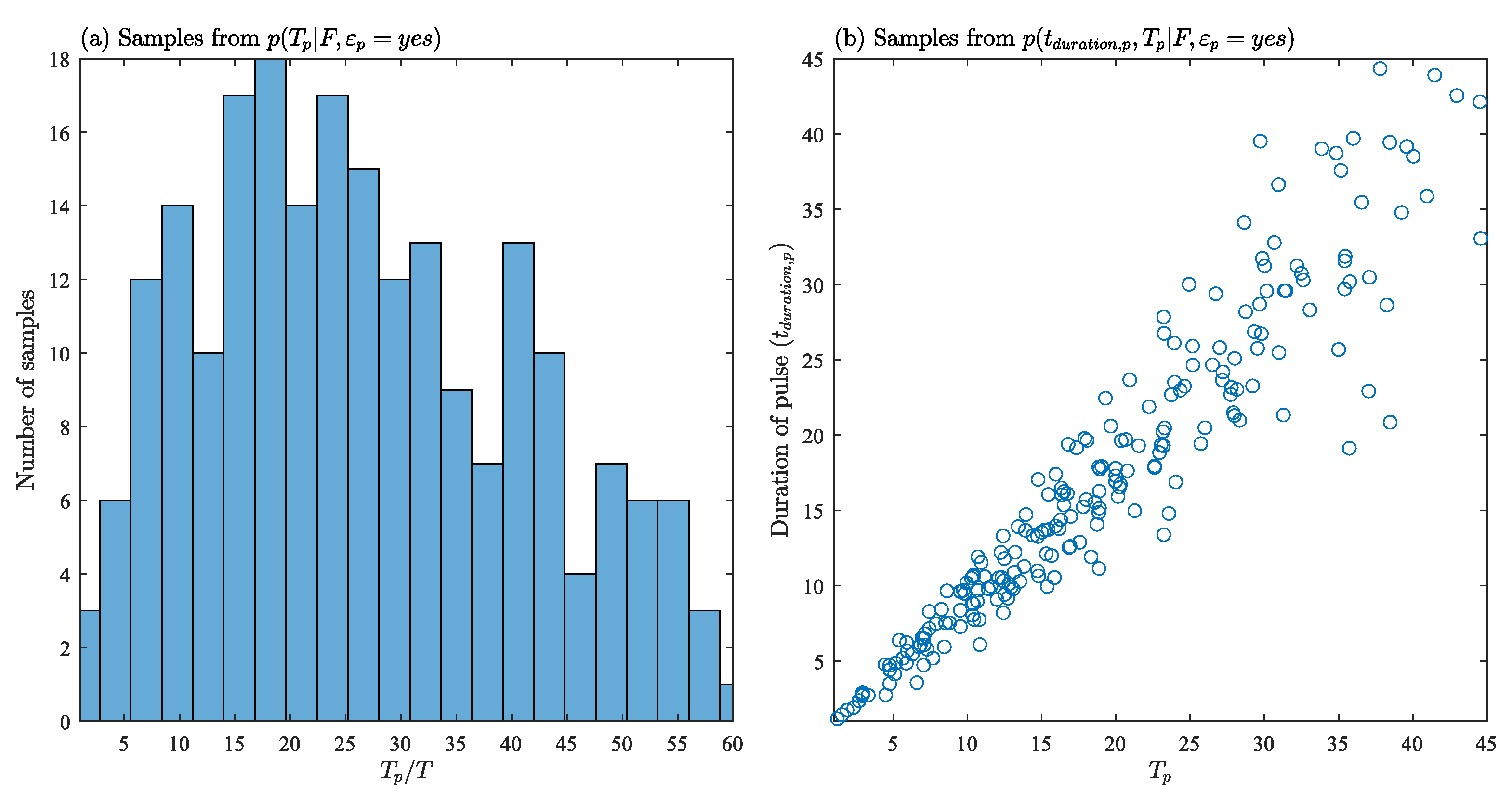
Appendix A.2. Long-Period Pulse

To describe the pulse characteristics of the near-fault ground motion, the mathematical model in [24] for the velocity pulse is used,
V = A p 2 [ 1 + cos ( 2 π f p γ p ( t t o ) ) ] cos ( 2 π f p ( t t o ) + ν p ) t [ t o γ p / 2 f p , t o + γ p / 2 f p ] ; = 0 otherwise
where A p is the signal amplitude, f p the dominating frequency, v p the phase angle, γ p the number of half cycles, and t o the time shift. These parameters can be related to the seismicity characteristics such as moment magnitude M or rupture distance r. Based on recommendations in [53,54], the pulse amplitude A p and period T p can be established through the following predictive relationships
A p = I p 10 0.9 ( 2.04 0.032 r + e A p ) ; T p = 10 2.9 + 0.5 M + e T p
where e A p and e T p are zero mean Gaussian variables with standard deviations 0.187 and 0.143, respectively, and I p is the indicator function describing whether the pulse exists or not. The probability models for γ p is chosen as Gaussian with mean 1.8 and standard deviation 0.3, while v p is assumed to follow an uniform distribution between [ 0 , π ] [19].
Since not all near-fault excitations will have a velocity pulse, the probability of pulse occurrence needs to be integrated in the stochastic model as well. This is established by introducing a discrete random variable ε p with outcomes as either yes or no. The probability of having pulse (i.e., probability of ε p = y e s ) can be estimated as a function related to the seismicity characteristics. For strike-slip faults, the probabilistic model in [25] is used to predict this probability,
P ( ε p = y e s | r , s ) = 1 1 + exp ( 0.642 + 0.167 r 0.075 s )
where r is the rupture distance and s is the distance between epicenter and site projection on the fault plane surface. s is taken as 1/4 of the total length of rupture L following the simplified process in [55]. L is established by the predictive equation [56] log 10 ( L ) = 3.55 + 0.74 M + e L , where e L is a zero mean Gaussian variable with standard deviation of 0.23. In the end, if ε p = y e s , then there is pulse and I p = 1 , otherwise, if ε p = n o , then I p = 0 . Similar to the high frequency component of the excitation, the uncertain model parameters that characterize the long-period pulse are taken as θ p = { e A p , e T p , γ p , v p , e L , ε p } , which are independent from the remaining seismic hazard characteristics [19].

References

  1. Comartin, C.D.; Niewiarowski, R.W.; Freeman, S.A.; Turner, F.M. Seismic evaluation and retrofit of concrete buildings: A practical overview of the ATC 40 Document. Earthq. Spectra 2000, 16, 241–261. [Google Scholar] [CrossRef]
  2. FEMA. Improvement of Nonlinear Static Seismic Analysis Procedures; Technical Report 440; Federal Emergency Management Agency: Washington, DC, USA, 2005.
  3. FEMA. Techniques for the Seismic Rehabilitation of Existing Buildings; Technical Report 547; Federal Emergency Management Agency: Washington, DC, USA, 2006.
  4. Chen, C.H. Performance-Based Seismic Demand Assessment of Concentrically Braced Steel Frame Buildings. Ph.D. Thesis, University of California, Berkeley, CA, USA, 2012. [Google Scholar]
  5. Sabelli, R.; Roeder, C.W.; Hajjar, J.F. Seismic Design of Steel Special Concentrically Braced Frame Systems—A Guide for Practicing Engineers. In NEHRP Seismic Design Technical Brief; NIST: Gaithersburg, MA, USA, 2013; pp. 1–36. [Google Scholar]
  6. Liel, A.B.; Haselton, C.B.; Deierlein, G.G. Seismic Collapse Safety of Reinforced Concrete Buildings. II: Comparative Assessment of Nonductile and Ductile Moment Frames. J. Struct. Eng. 2011, 137, 492–502. [Google Scholar] [CrossRef]
  7. Astaneh-Asl, A.; Cochran, M.; Sabelli, R. Seismic detailing of gusset plates for special concentrically braced frames. In Structural Steel Educational Council; Steel TIPS: Moraga, CA, USA, 2006. [Google Scholar]
  8. Roeder, C.W.; Lehman, D.E.; Lumpkin, E.; Palmer, K. SCBF Gusset Plate Connection Design. In Proceedings of the North American Structural Steel Construction Conference, Pittsburgh, PA, USA, 10–14 May 2011. [Google Scholar]
  9. Roeder, C.W.; Lumpkin, E.J.; Lehman, D.E. A balanced design procedure for special concentrically braced frame connections. J. Constr. Steel Res. 2011, 67, 1760–1772. [Google Scholar] [CrossRef]
  10. Hsiao, P.C.; Lehman, D.E.; Roeder, C.W. Improved analytical model for special concentrically braced frames. J. Constr. Steel Res. 2012, 73, 80–94. [Google Scholar] [CrossRef]
  11. Palmer, K.D. Seismic Behavior, Performance and Design of Steel Concentrically Braced Frame Systems. Ph.D. Thesis, University of Washington, Seattle, WA, USA, 2012. [Google Scholar]
  12. Hammad, A. Seismic Behavior of Special Concentric Braced Frames under Long Duration Ground Motions. Ph.D. Thesis, University of Nevada, Reno, NV, USA, 2019. [Google Scholar]
  13. Vafaei, D.; Shemshadian, M.; Zahrai, S. Seismic behavior of BRB frames under near fault excitations. In Proceedings of the 9th US National and 10th Canadian Conference on Earthquake Engineering, Toronto, ON, Canada, 25–29 July 2010. [Google Scholar]
  14. Alavi, B.; Krawinkler, H. Behavior of moment-resisting frame structures subjected to near-fault ground motions. Earthq. Eng. Struct. Dyn. 2004, 33, 687–706. [Google Scholar] [CrossRef]
  15. Liel, A.B.; Haselton, C.B.; Deierlein, G.G.; Baker, J.W. Incorporating modeling uncertainties in the assessment of seismic collapse risk of buildings. Struct. Saf. 2009, 31, 197–211. [Google Scholar] [CrossRef]
  16. Taflanidis, A.A.; Jia, G. A simulation-based framework for risk assessment and probabilistic sensitivity analysis of base-isolated structures. Earthq. Eng. Struct. Dyn. 2011, 40, 1629–1651. [Google Scholar] [CrossRef]
  17. Liel, A.B.; Deierlein, G.G. Using Collapse Risk Assessments to Inform Seismic Safety Policy for Older Concrete Buildings. Earthq. Spectra 2012, 28, 1495–1521. [Google Scholar] [CrossRef]
  18. Champion, C.; Liel, A.B. The effect of near-fault directivity on building seismic collapse risk. Earthq. Eng. Struct. Dyn. 2012, 41, 1391–1409. [Google Scholar] [CrossRef]
  19. Jia, G.; Gidaris, I.; Taflanidis, A.A.; Mavroeidis, G.P. Reliability-based assessment/design of floor isolation systems. Eng. Struct. 2014, 78, 41–56. [Google Scholar] [CrossRef]
  20. Vamvatsikos, D.; Cornell, C.A. The incremental dynamic analysis and its application to performance-based earthquake engineering. In Proceedings of the 12th European Conference on Earthquake Engineering, London, UK, 9–13 September 2002. [Google Scholar]
  21. Vamvatsikos, D.; Cornell, C.A. Direct estimation of seismic demand and capacity of multidegree-of-freedom systems through incremental dynamic analysis of single degree of freedom approximation. J. Struct. Eng. 2005, 131, 589–599. [Google Scholar] [CrossRef] [Green Version]
  22. Song, R.; Li, Y.; van de Lindt, J.W. Impact of earthquake ground motion characteristics on collapse risk of post-mainshock buildings considering aftershocks. Eng. Struct. 2014, 81, 349–361. [Google Scholar] [CrossRef]
  23. Li, Y.; Song, R.; Van De Lindt, J.W. Collapse fragility of steel structures subjected to earthquake mainshock-aftershock sequences. J. Struct. Eng. 2014, 140, 1–10. [Google Scholar] [CrossRef]
  24. Mavroeidis, G.; Papageorgiou, A. A mathematical representation of near-fault ground motions. Bull. Seismol. 2003, 93, 1099–1131. [Google Scholar] [CrossRef]
  25. Shahi, S.K.; Baker, J.W. An empirically calibrated framework for including the effects of near-fault directivity in probabilistic seismic hazard analysis. Bull. Seismol. Soc. Am. 2011, 101, 742–755. [Google Scholar] [CrossRef]
  26. Robert, C.P.; Casella, G. Monte Carlo Statistical Methods, 2nd ed.; Springer: New York, NY, USA, 2004. [Google Scholar]
  27. Au, S.K.; Beck, J.L. Estimation of small failure probabilities in high dimensions by subset simulation. Probabilistic Eng. Mech. 2001, 16, 263–277. [Google Scholar] [CrossRef] [Green Version]
  28. Jia, G.; Taflanidis, A.A.; Beck, J.L. A new adaptive rejection sampling method using kernel density approximations and its application to Subset Simulation. ASCE ASME J. Risk Uncertain. Eng. Syst. Part A Civ. Eng. 2017, 3, D4015001. [Google Scholar] [CrossRef]
  29. Jia, G.; Tabandeh, A.; Gardoni, P. A density extrapolation approach to estimate failure probabilities. Struct. Saf. 2021, 93, 102128. [Google Scholar] [CrossRef]
  30. Karunamuni, R.; Zhang, S. Some improvements on a boundary corrected kernel density estimator. Stat. Probab. Lett. 2008, 78, 499–507. [Google Scholar] [CrossRef]
  31. Jia, G.; Taflanidis, A.A. Sample-based evaluation of global probabilistic sensitivity measures. Comput. Struct. 2014, 144, 103–118. [Google Scholar] [CrossRef]
  32. FEMA. State of the Art Report on Systems Performance of Steel Moment Frames Subject to Earthquake Ground Shaking; Technical Report 355; Federal Emergency Management Agency: Washington, DC, USA, 2000.
  33. Rafn Gunnarsson, I. Numerical Performance Evaluation of Braced Frame Systems. Master’s Thesis, University of Washington, Seattle, WA, USA, 2004. [Google Scholar]
  34. Bruneau, M.; Uang, C.M.; Sabelli, R. Ductile Design of Steel Structures, 2nd ed.; McGraw Hill Education: New York, NY, USA, 2011. [Google Scholar]
  35. Khatib, I.F.; Mahin, S.A.; Pister, K.S. Seismic Behavior of Concentrically Braced Steel Frames; Technical Report, UCB/EERC-88/01; University of California: Berkeley, CA, USA, 1988. [Google Scholar]
  36. Leon, R.T.; Yang, C.S. Special inverted-V-braced frames with suspended zipper struts. In Proceedings of the International Workshop on Steel and Concrete Composite Construction, Taipei, Taiwan, 8–9 October 2003. [Google Scholar]
  37. Yang, C.S. Analytical and Experimental Study of Concentrically Braced Frames with Zipper Struts. Ph.D. Thesis, Georgia Institute of Technology, Atlanta, GA, USA, 2006. [Google Scholar]
  38. Elnashai, A.; Papanikolaou, V.; Lee, D. Zeus NL—A System for Inelastic Analysis of Structures; Technical Report; Mid-America Earthquake Center, University of Illinois at Urbana-Champaign: Champaign, IL, USA, 2004. [Google Scholar]
  39. Karamanci, E.; Lignos, D.G. Computational approach for collapse assessment of concentrically braced frames in seismic regions. J. Struct. Eng. 2014, 140, A4014019. [Google Scholar] [CrossRef]
  40. Terzic, V. Discovering OpenSees—Modeling SCB Frames Using Beam-Column Elements; Open System for Earthquake Engineering Simulation: Berkeley, CA, USA, 2013. [Google Scholar]
  41. Uriz, P.; Mahin, S.A. Seismic performance assessment of concentrically braced steel frames. In Proceedings of the 13th World Conference on Earthquake Engineering, Vancouver, BC, Canada, 1–6 August 2004; p. 6. [Google Scholar]
  42. Uriz, P. Towards Earthquake Resistant Design of Concentrically Braced Steel Structures; University of California: Berkeley, CA, USA, 2005. [Google Scholar]
  43. Hsiao, P.C.; Lehman, D.E.; Roeder, C.W. A model to simulate special concentrically braced frames beyond brace fracture. Earthq. Eng. Struct. Dyn. 2013, 42, 183–200. [Google Scholar] [CrossRef]
  44. Tirca, L.; Chen, L. Numerical simulation of inelastic cyclic response of HSS braces upon fracture. Adv. Steel Constr. 2014, 10, 442–462. [Google Scholar]
  45. Wen, H.; Mahmoud, H. New Model for Ductile Fracture of Metal Alloys. I: Monotonic Loading. J. Eng. Mech. 2016, 142, 04015088. [Google Scholar] [CrossRef]
  46. Hammad, A.; Moustafa, M.A. Modeling sensitivity analysis of special concentrically braced frames under short and long duration ground motions. Soil Dyn. Earthq. Eng. 2020, 128, 105867. [Google Scholar] [CrossRef]
  47. Hammad, A.; Moustafa, M.A. Numerical analysis of special concentric braced frames using experimentally-validated fatigue and fracture model under short and long duration earthquakes. Bull. Earthq. Eng. 2021, 19, 287–316. [Google Scholar] [CrossRef]
  48. Atkinson, G.; Silva, W. Stochastic modeling of California ground motions. Bull. Seismol. Soc. Am. 2000, 90, 255–274. [Google Scholar] [CrossRef]
  49. Atkinson, G.M. Ground-motion prediction equations for eastern North America from a referenced empirical approach: Implications for epistemic uncertainty. Bull. Seismol. Soc. Am. 2008, 98, 1304–1318. [Google Scholar] [CrossRef]
  50. Vetter, C.; Taflanidis, A.A. Comparison of alternative stochastic ground motion models for seismic risk characterization. Soil Dyn. Earthq. Eng. 2014, 58, 48–65. [Google Scholar] [CrossRef]
  51. Vetter, C.; Taflanidis, A.A. Global sensitivity analysis for stochastic ground motion modeling in seismic-risk assessment. Soil Dyn. Earthq. Eng. 2012, 38, 128–143. [Google Scholar] [CrossRef]
  52. Boore, D.M. Simulation of Ground Motion Using the Stochastic Method. Pure Appl. Geophys. 2003, 160, 635–676. [Google Scholar] [CrossRef] [Green Version]
  53. Bray, J.D.; Rodriguez-Marek, A. Characterization of forward-directivity ground motions in the near-fault region. Soil Dyn. Earthq. Eng. 2004, 24, 815–828. [Google Scholar] [CrossRef]
  54. Halldórsson, B.; Mavroeidis, G.P.; Papageorgiou, A.S. Near-fault and far-field strong ground-motion simulation for earthquake engineering applications using the specific barrier model. J. Struct. Eng. 2010, 137, 433–444. [Google Scholar] [CrossRef]
  55. Gidaris, I.; Taflanidis, A.A. Performance assessment and optimization of fluid viscous dampers through life-cycle cost criteria and comparison to alternative design approaches. Bull. Earthq. Eng. 2015, 13, 1003–1028. [Google Scholar] [CrossRef]
  56. Wells, D.L.; Coppersmith, K.J. New empirical relationships among magnitude, rupture length, rupture width, rupture area, and surface displacement. Bull. Seismol. Soc. Am. 1994, 84, 974–1002. [Google Scholar]
Figure 1. Augmented system model for seismic collapse risk quantification.
Metals 11 01271 g001
Figure 2. Illustration of the stochastic near-fault ground motion model and sample ground motion time history.
Metals 11 01271 g002
Figure 3. Flowchart for simulation based approach for seismic collapse risk assessment and probabilistic sensitivity analysis.
Metals 11 01271 g003
Figure 4. Floor plan and elevation view of the three-story SAC building.
Metals 11 01271 g004
Figure 5. Configuration of (a) the chevron-braced frame and (b) the cross-braced frame.
Metals 11 01271 g005
Figure 6. Visualization of joint element and imperfection in braces.
Metals 11 01271 g006
Figure 7. Pushover curves for the braced frames.
Metals 11 01271 g007
Figure 8. Axial force-axial displacement for the braces in the chevron-braced frame.
Metals 11 01271 g008
Figure 9. Hysteretic behavior of the chevron-braced frame.
Metals 11 01271 g009
Figure 10. Axial force-axial displacement for the braces in the cross-braced frame.
Metals 11 01271 g010
Figure 11. Hysteretic behavior of the cross-braced frame.
Metals 11 01271 g011
Figure 12. Seismic risk for the two frames under different performance thresholds, where for (a) the failure definition also includes the failure due to low-cycle fatigue, and for (b) the failure definition does not include the failure due to low-cycle fatigue.
Metals 11 01271 g012
Figure 13. Samples from (a) p ( M , r ) , (b) p ( M , r | F ) , (c) p ( M , r | F , ε p = y e s ) , and (d) p ( M , r | F , ε p = n o ) . All the plots are for chevron-braced frame.
Metals 11 01271 g013
Figure 14. Samples from (a) p ( S a ,   P G V ) , (b) p ( S a ,   P G V | F ) , (c) p ( S a ,   P G V | F , ε p = y e s ) , and (d) p ( S a ,   P G V | F , ε p = n o ) . All the plots are for chevron-braced frame.
Metals 11 01271 g014
Figure 15. (a) Samples for ratio of pulse period to fundamental period of structure conditional on failure and ε p = y e s (i.e., samples from p ( T p | F , ε p = y e s ) ). (b) Samples for pulse period and pulse duration conditional on failure and ε p = y e s (i.e., samples from p ( T p , t d u r a t i o n , p | F , ε p = y e s ) ). Both plots are for the chevron-braced frame.
Metals 11 01271 g015
Figure 16. Samples from (a) p ( M ,   r ) , (b) p ( M ,   r | F ) , (c) p ( M ,   r | F , ε p = y e s ) , and (d) p ( M ,   r | F , ε p = n o ) . All plots are for cross-braced frame.
Metals 11 01271 g016
Figure 17. Samples from (a) p ( S a ,   P G V ) , (b) p ( S a ,   P G V | F ) , (c) p ( S a ,   P G V | F , ε p   =   y e s ) , and (d) p ( S a ,   P G V | F , ε p   =   n o ) . All plots are for cross-braced frame.
Metals 11 01271 g017
Figure 18. (a) Samples for ratio of pulse period to fundamental period of structure conditional on failure and ε p   =   y e s (i.e., samples from p ( T p | F , ε p   =   y e s ) ). (b) Samples for pulse period and pulse duration conditional on failure and ε p   =   y e s (i.e., samples from p ( T p , t d u r a t i o n , p | F , ε p   =   y e s ) ). Both are for the cross-braced frame.
Metals 11 01271 g018
Table 1. Failure probability of braced frames corresponding to different damage states (in %).
Damage
State
Chevron-Braced FrameCross-Braced Frame
P ( F | ε p = yes , no ) P ( F | ε p = no ) P ( F | ε p = yes , no ) P ( F | ε p = no )
‘Slight’34.7326.6356.1645.99
‘Moderate’8.895.5020.6514.64
‘Extensive’0.550.104.541.86
‘Collapse’0.430.053.921.11
Table 2. Probabilistic sensitivity analysis results for ground motion with probabilistic pulse and no pulse for chevron-braced frame.
Independent
Parameters
Relative EntropyResultant
Parameters
Relative Entropy
ε p = { yes , no } ε p = { no } ε p = { yes , no } ε p = { no }
M3.2012.806 S a 3.7654.053
r0.4810.279 P G V 3.0513.129
e b 0.3390.555 f a 2.7722.131
e e 0.1030.109 f b 2.5762.005
ε p 1.493 e2.3801.791
e A p 0.050 T p 2.109
e T p 0.003 L1.721
[ M ,   r ] 3.8533.286 A p 0.445
[ M ,   e T p ] 3.074
[ r ,   e A p ] 0.572
Table 3. Probabilistic sensitivity analysis results for ground motion with probabilistic pulse and no pulse for cross-braced frame.
Independent ParametersRelative EntropyResultant ParametersRelative Entropy
ε p = { yes , no } ε p = { no } ε p = { yes , no } ε p = { no }
M1.7492.055 S a 2.6102.928
r0.4320.098 P G V 2.6202.199
e b 0.0840.315 f a 1.4891.803
e e 0.0490.137 f b 1.3861.498
ε p 0.983 e1.1851.141
e A p 0.066 T p 1.269
e T p 0.014 L1.243
[ M , r ] 2.3702.235 A p 0.441
[ M , e T p ] 1.770
[ r , e A p ] 0.496
Publisher’s Note: MDPI stays neutral with regard to jurisdictional claims in published maps and institutional affiliations.

