
Forecasting Model of Silicon Content in Molten Iron Using Wavelet Decomposition and Artificial Neural Networks

 , ,
, , 
Abstract
:1. Introduction
2. The Blast Furnace Process
2.1. Background
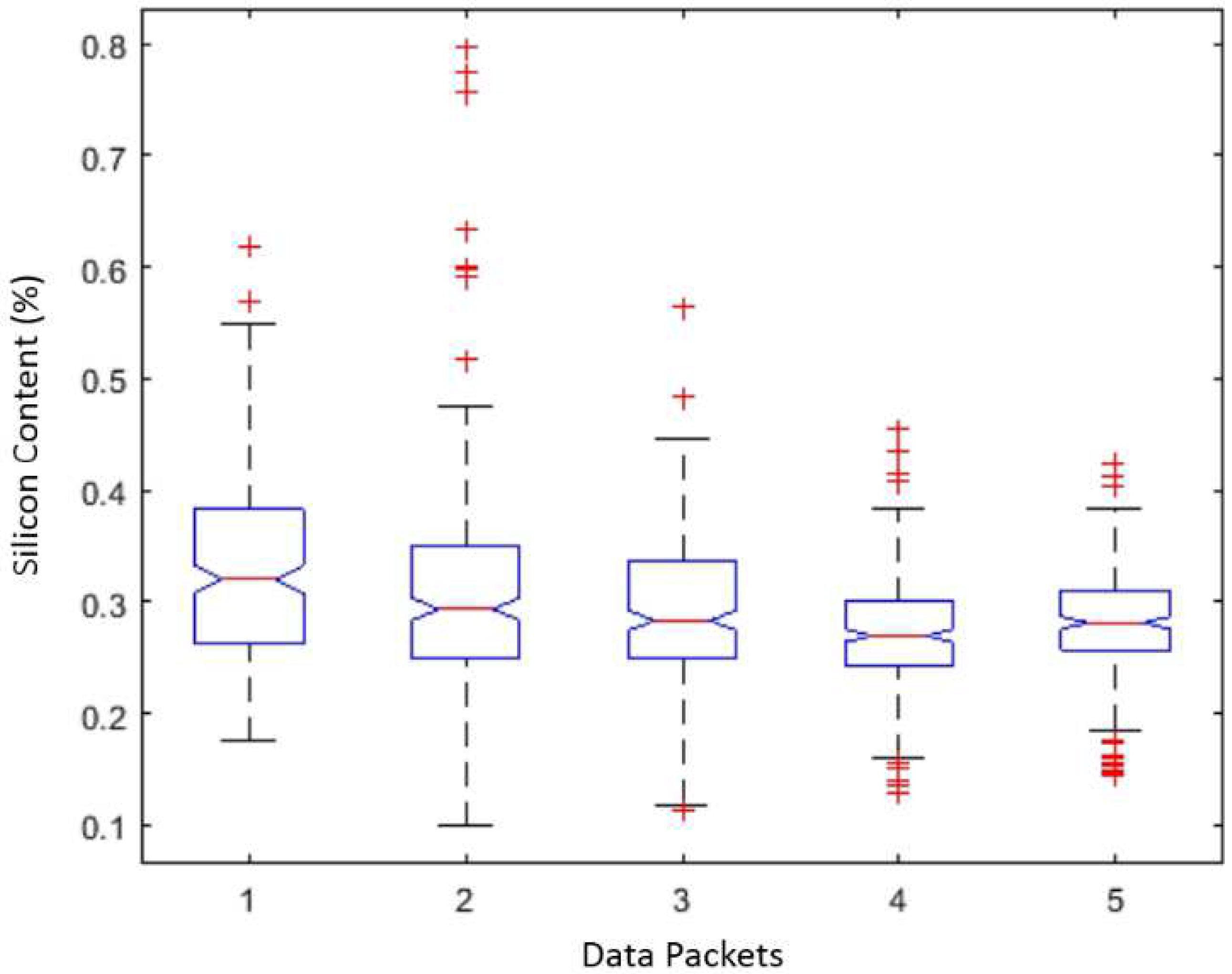
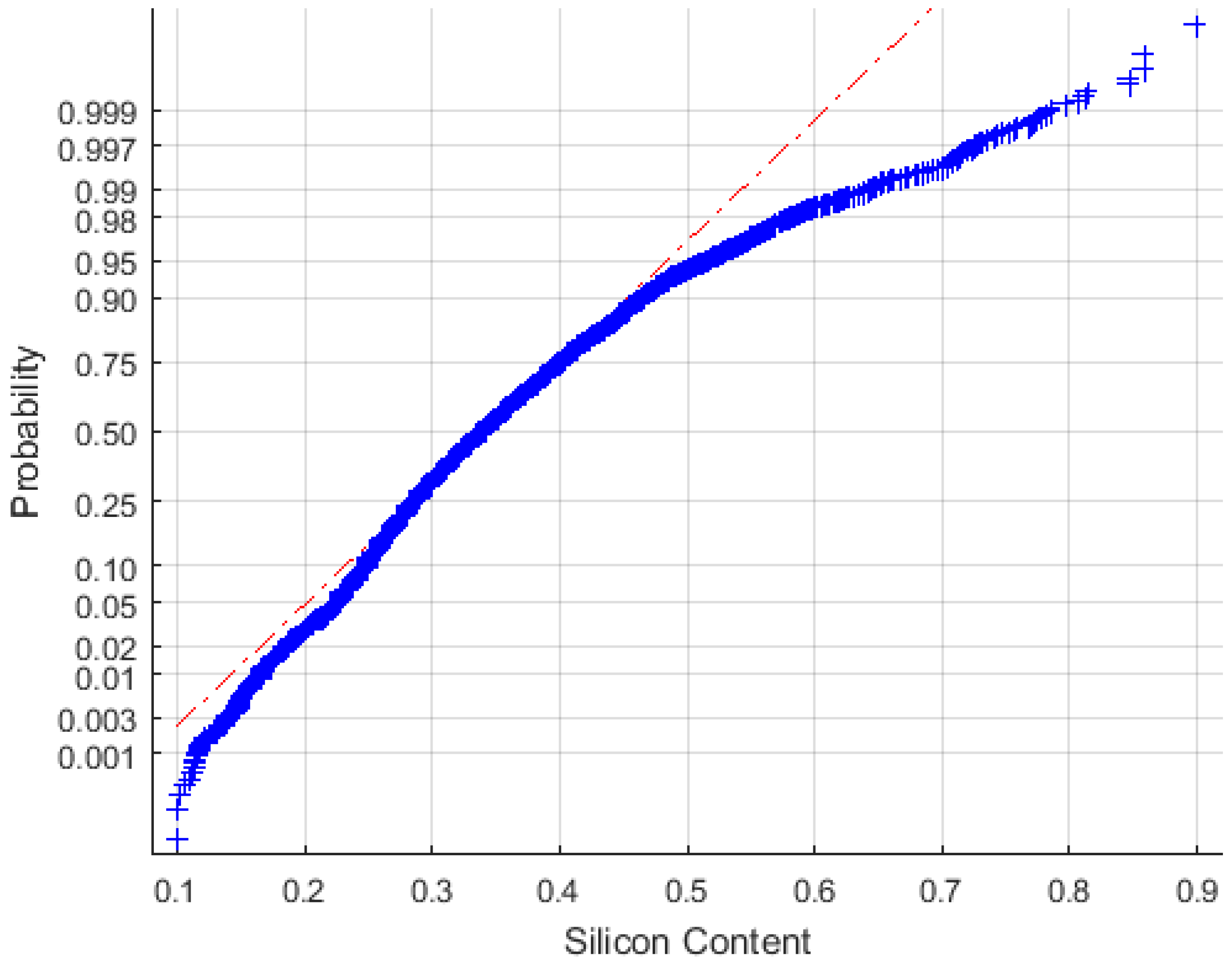
2.2. The Dataset
3. Silicon Content Time Series Modeling
3.1. NIO, NARX, and NAR Neural Network Models
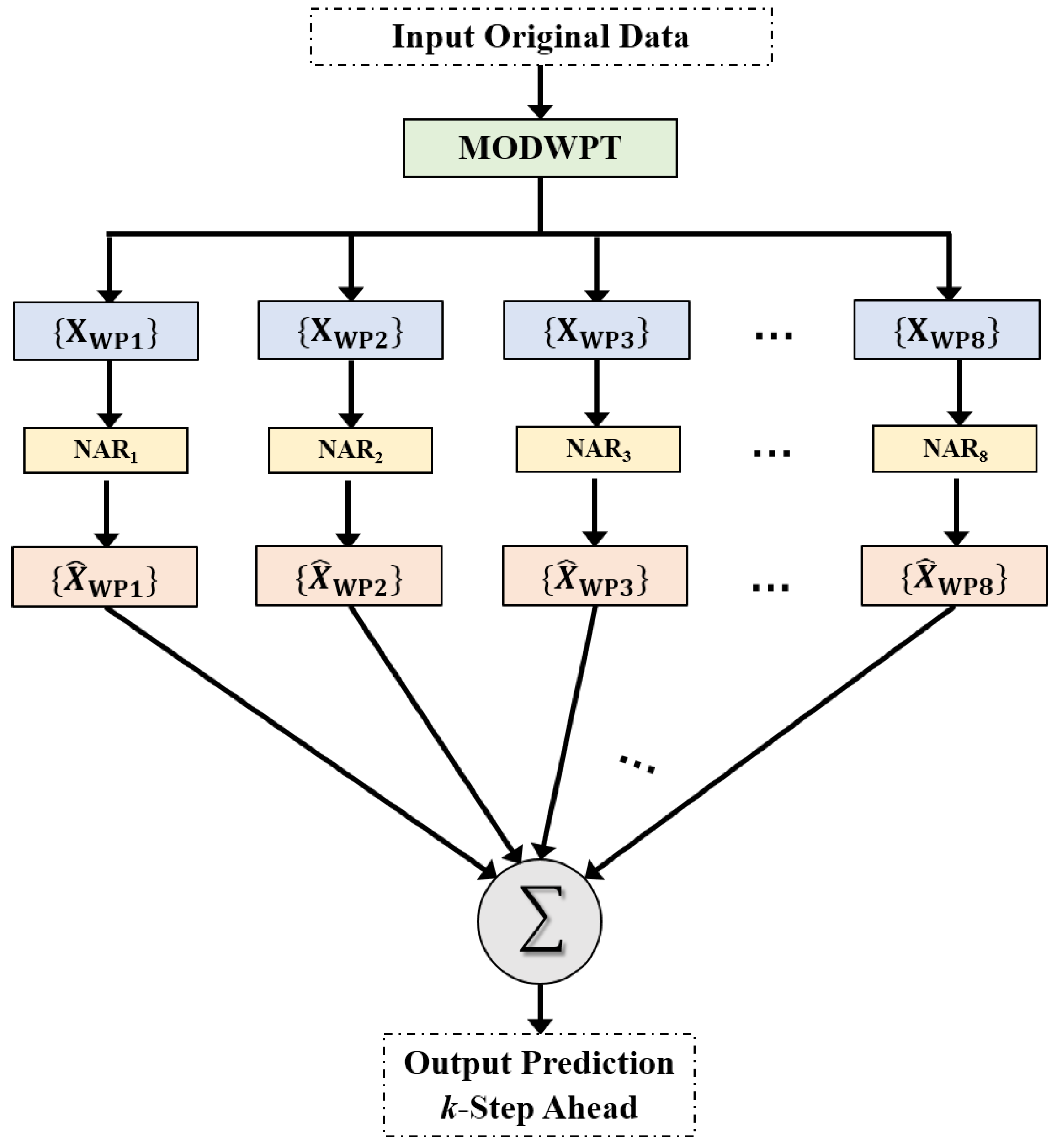
3.2. MODWPT-NAR Neural Network Model
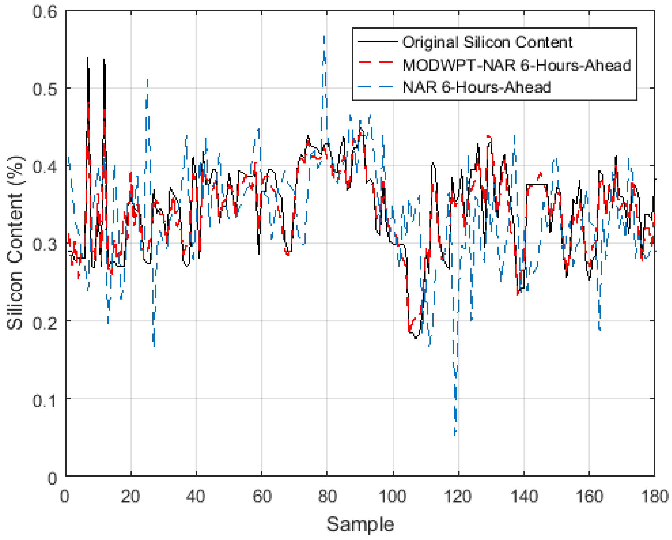
4. Comparative Analysis of Forecasting Models
5. Conclusions
Author Contributions
Funding
Data Availability Statement
Acknowledgments
Conflicts of Interest
References
- Li, H.; Bu, X.; Liu, X.; Li, X.; Li, H.; Liu, F.; Lyu, Q. Evaluation and Prediction of Blast Furnace Status Based on Big Data Platform of Ironmaking and Data Mining. ISIJ Int. 2021, 61, 108–118. [Google Scholar] [CrossRef]
- Geerdes, M.D.; Toxopeus, H.; Vliet, C.; Young, G.O. Modern Blast Furnace Ironmaking: An Introduction; IOS Press BV: Amsterdam, The Netherlands, 2009. [Google Scholar]
- Gomes, F.S.V.; Coco, K.F.; Salles, J.L.F. Multistep forecasting models of the liquid level in a blast furnace hearth. IEEE Trans. Autom. Sci. 2017, 14, 1286–1296. [Google Scholar] [CrossRef]
- Singh, H.; Sridhar, N.V.; Deo, B. Artificial neural nets for prediction of silicon content of blast furnace hot metal. Steel Res. Int. 1996, 67, 521–527. [Google Scholar] [CrossRef]
- Chen, J. A predictive system for blast furnaces by integrating a neural network with qualitative analysis. Eng. Appl. Artif. Intell. 2001, 14, 77–85. [Google Scholar] [CrossRef]
- Saxén, H.; Pettersson, F. Nonlinear prediction of the hot metal silicon content in the blast furnace. ISIJ Int. 2007, 47, 1732–1737. [Google Scholar] [CrossRef] [Green Version]
- Nurkkala, A.; Pettersson, F.; Saxén, H. Non linear modeling method applied to prediction of hot metal silicon in the ironmaking blast furnace. Ind. Eng. Chem. Res. 2011, 50, 9236–9248. [Google Scholar] [CrossRef]
- Saxén, H.; Gao, C.; Gao, Z. Data-Driven Time Discrete Models for Dynamic Prediction of the Hot Metal Silicon Content in the Blast Furnace—A Review. IEEE Trans. Ind. Inform. 2013, 9, 2213–2225. [Google Scholar] [CrossRef]
- Chen, W.; Wang, B.X.; Han, H.L. Prediction and control for silicon content in pig iron of blast furnace by integrating artificial neural network with genetic algorithm. Ironmak. Steelmak. 2010, 37, 458–463. [Google Scholar] [CrossRef]
- Wang, H.; Yang, G.; Pan, C.; Gong, Q. Prediction of hot metal silicon content in blast furnace based on EMD and DNN. In Proceedings of the 34th Chinese Control Conference, Hangzhou, China, 28–30 July 2015; pp. 8214–8218. [Google Scholar]
- Zhang, H.; Zhang, S.; Yin, Y.; Chen, X. Prediction of the hot metal silicon content in blast furnace based on extreme learning machine. Int. J. Mach. Learn. Cybern. 2017, 9, 697–1706. [Google Scholar] [CrossRef]
- Su, X.; Zhang, S.; Yin, Y.; Hui, Y.; Xiao, W. Prediction of hot metal silicon content for blast furnace based on multi-layer online sequential extreme learning machine. In Proceedings of the 37th Chinese Control Conference (CCC), Wuhan, China, 25–27 July 2018; pp. 8025–8030. [Google Scholar]
- Saxén, H.; Pettersson, F. Method for the selection of inputs and structure of feedforward neural networks. Comput. Chem. Eng. 2006, 30, 1038–1045. [Google Scholar] [CrossRef]
- Cao, J.; Lin, Z.; Huang, G.B. Self-adaptive evolutionary extreme learning machine. Neural Process. Lett. 2012, 36, 285–305. [Google Scholar] [CrossRef]
- Chazal, P.; Tapson, J.; Schaik, A.V. A comparison of extreme learning machines and backpropagation trained feed-forward networks processing the mnist database. In Proceedings of the 2015 IEEE International Conference on Acoustics, Speech and Signal Processing (ICASSP), South Brisbane, QLD, Australia, 19–24 April 2015; pp. 2165–2168. [Google Scholar]
- Percival, D.B.; Walden, A.T. Wavelet Methods for Time Series Analysis; Cambridge University Press: Cambridge, UK, 2000. [Google Scholar]
- Walden, A.T.; Cristan, A.C. The phase-corrected undecimated discrete wavelet packet transform and its application to interpreting the timing of events. Proc. R. Soc. Lond. 1998, 454, 2243–2266. [Google Scholar] [CrossRef]
- Su, X.; Zhen, S.; Yin, Y.; Xiao, W. Prediction model of permeability index for blast furnace based on the improved multi-layer extreme learn machine and wavelet transform. J. Frankl. Inst. 2018, 355, 1663–1691. [Google Scholar] [CrossRef]
- Labate, D.; Foresta, F.L.; Occhiuto, G.; Morabito, F.C.; Lay-Ekuakille, A.; Vergallo, P. EMD vs. DWT for the extraction of respiratory signal from single-channel ECG: A comparison. IEEE Sens. J. 2013, 13, 2666–2674. [Google Scholar] [CrossRef]
- Saxén, H. Short-term prediction of silicon content in pig iron. Can. Metall. Q. 1994, 33, 319–326. [Google Scholar] [CrossRef]
- Zhou, B.; Ye, H.; Zhang, H.; Li, M. Process monotoring of iron-making process with PCA-based methods. Control Eng. Pract. 2016, 47, 1–14. [Google Scholar] [CrossRef]
- Kwiatkowski, D.; Phillips, P.C.B.; Schmidt, P.; Shin, Y. Testing the null hypothesis of stationarity against the alternative of a unit root. J. Econom. 1982, 54, 159–178. [Google Scholar] [CrossRef]
- Lilliefors, H.W. On the Kolmogorov–Smirnov test for normality with mean and variance unknown. J. Am. Stat. Assoc. 1967, 62, 399–402. [Google Scholar] [CrossRef]
- Kruskal, W.; Wallis, W.A. Use of ranks in one-criterion variance analysis. J. Am. Stat. Assoc. 1952, 47, 583–621. [Google Scholar] [CrossRef]
- Haykin, S. Neural Networks and Learning Machines; Pearson Education, Inc.: Upper Saddle River, NJ, USA, 2009. [Google Scholar]
- Hu, Y.H.; Hwang, J. Handbook of Neural Network Signal Processing; CRC Press: Boca Raton, FL, USA, 2002. [Google Scholar]
- Mallat, S. A Wavelet Tour of Signal Processing; Academic Press: Burlington, MA, USA, 2008. [Google Scholar]
- Hassibi, B.; Stork, D.G.; Wolff, G. Optimal Brain Surgeon and general network pruning. In Proceedings of the IEEE International Conference on Neural Networks, San Francisco, CA, USA, 28 March–1 April 1993; pp. 293–299. [Google Scholar]
- The NNSYSID Toolbox-a MATLAB(R) Toolbox for System Identification with Neural Networks. Available online: https://www.mathworks.com/matlabcentral/fileexchange/87-nnsysid (accessed on 18 May 2021).


| Variable | Description |
|---|---|
| flame temperature (°C) | |
| rate of CO/CO2 | |
| H2 gas efficiency (%) | |
| molten iron production (tons/min) | |
| coke rate (Kg/ton of molten iron) | |
| pulverized coal injection rate (Kg/ton of molten iron) | |
| direct reduction (%) | |
| ore/coke ratio | |
| thermal index of H0 ( Kcal/ton of molten iron) | |
| north central gaseous flow index | |
| north peripheral gaseous flow index | |
| south central gaseous flow index | |
| south peripheral gaseous flow index | |
| blowing air volume (Nm3/min) | |
| blowing air moisture (g/Nm3) | |
| blowing air temperature (°C) | |
| blowing air pressure (Kg/cm2) | |
| top pressure (Kg/cm2) | |
| top temperature (°C) | |
| composition of H2 on the top gas (%) | |
| composition of N2 on the top gas (%) | |
| composition of CO on the top gas (%) | |
| composition of CO2 on the top gas (%) | |
| O2 enrichment rate (%) | |
| CO efficiency (%) | |
| staves’ thermal losses ( Kcal/h) | |
| molten iron temperature | |
| electromotive force (%) |
| ANN Model | Regressors |
|---|---|
| NIO | |
| NARX | for |
| for | |
| for | |
| for | |
| NAR | for |
| Neural Network | Hidden Layer Size | MSE(0) () |
|---|---|---|
| NAR1 | 27 | 0.0169 |
| NAR2 | 8 | 0.2642 |
| NAR3 | 7 | 0.1299 |
| NAR4 | 19 | 0.0487 |
| NAR5 | 21 | 0.0500 |
| NAR6 | 25 | 0.0442 |
| NAR7 | 23 | 0.0708 |
| NAR8 | 14 | 0.0047 |
| Model | Horizon | MSE(k) | MAPE(k) | AEPϵ(k) |
|---|---|---|---|---|
| (k) | () | (%) | (%) | |
| NIO | 3 | 21.15 | 38.85 | 27.32 |
| 4 | 20.54 | 38.28 | 30.60 | |
| 5 | 20.29 | 38.05 | 30.90 | |
| 6 | 20.48 | 38.25 | 28.14 | |
| NARX | 3 | 13.42 | 32.15 | 33.80 |
| 4 | 11.65 | 29.55 | 36.53 | |
| 5 | 12.37 | 30.42 | 34.74 | |
| 6 | 11.87 | 29.04 | 36.63 | |
| NAR | 3 | 3.05 | 12.88 | 73.73 |
| 4 | 4.40 | 15.07 | 66.94 | |
| 5 | 9.07 | 21.76 | 53.80 | |
| 6 | 15.17 | 29.50 | 40.48 |
| Model | Horizon | MSE(k) | MAPE(k) | AEPϵ(k) |
|---|---|---|---|---|
| (k) | () | (%) | (%) | |
| NIO | 3 | 5.24 | 18.76 | 58.30 |
| 4 | 5.28 | 18.76 | 58.53 | |
| 5 | 5.38 | 18.74 | 60.02 | |
| 6 | 5.45 | 18.76 | 59.83 | |
| NARX | 3 | 5.31 | 17.98 | 56.33 |
| 4 | 5.67 | 18.82 | 54.58 | |
| 5 | 6.04 | 19.55 | 51.41 | |
| 6 | 6.40 | 20.13 | 49.50 | |
| NAR | 3 | 3.36 | 12.29 | 76.26 |
| 4 | 5.88 | 16.49 | 66.24 | |
| 5 | 15.31 | 26.26 | 52.53 | |
| 6 | 21.52 | 31.76 | 40.76 |
| Horizon | MSE(k) | MAPE(k) | |
|---|---|---|---|
| (k) | () | (%) | (%) |
| 3 | 0.043 | 1.58 | 100 |
| 4 | 0.14 | 2.82 | 99.72 |
| 5 | 0.22 | 3.54 | 99.02 |
| 6 | 0.30 | 4.21 | 98.18 |
| 7 | 0.33 | 4.54 | 97.90 |
| 8 | 0.83 | 6.57 | 93.70 |
Publisher’s Note: MDPI stays neutral with regard to jurisdictional claims in published maps and institutional affiliations. |
© 2021 by the authors. Licensee MDPI, Basel, Switzerland. This article is an open access article distributed under the terms and conditions of the Creative Commons Attribution (CC BY) license (https://creativecommons.org/licenses/by/4.0/).
Share and Cite
Diniz, A.P.M.; Côco, K.F.; Gomes, F.S.V.; Salles, J.L.F. Forecasting Model of Silicon Content in Molten Iron Using Wavelet Decomposition and Artificial Neural Networks. Metals 2021, 11, 1001. https://doi.org/10.3390/met11071001
Diniz APM, Côco KF, Gomes FSV, Salles JLF. Forecasting Model of Silicon Content in Molten Iron Using Wavelet Decomposition and Artificial Neural Networks. Metals. 2021; 11(7):1001. https://doi.org/10.3390/met11071001
Chicago/Turabian StyleDiniz, Ana P. Miranda, Klaus Fabian Côco, Flávio S. Vitorino Gomes, and José L. Félix Salles. 2021. "Forecasting Model of Silicon Content in Molten Iron Using Wavelet Decomposition and Artificial Neural Networks" Metals 11, no. 7: 1001. https://doi.org/10.3390/met11071001
APA StyleDiniz, A. P. M., Côco, K. F., Gomes, F. S. V., & Salles, J. L. F. (2021). Forecasting Model of Silicon Content in Molten Iron Using Wavelet Decomposition and Artificial Neural Networks. Metals, 11(7), 1001. https://doi.org/10.3390/met11071001