A New Approach to Calculate the Velocity of Interdendritic Fluid Flow during Solidification Using Etched Surface Height of Actual Metal Ingot

Abstract

Macrosegregation remains one of main defects affecting metal materials properties, which is mainly caused by interdendritic fluid flow during solidifying. However, as for controlling actual specific segregation, it is still difficult to effectively measure or simulate this kind flow instead of pure fluid flow, especially in complex casting processes of high-grade materials. Herein, a new method for obtaining velocity magnitude and direction of interdendritic fluid flow during metal solidifying is proposed from boundary layer and standard deviation obtained by measuring etched surface heights of the actual ingot and using statistical principles. Taking continuous casting bloom of GCr15 bearing steel as an example, it is indicated that the calculated velocity magnitudes under different sides and superheats can be explained by process features and, hence, solidification mechanism. The velocity magnitude and fluctuation are higher on the inner curve side and under low superheat. Meanwhile, it is found that the fluctuation extent of secondary arm spacing is more relevant with interdendritic fluid flow, although its magnitude is mainly determined by the cooling rate. Moreover, on the basis of the calculated velocity directions and magnitudes, there is a positive correlation between segregation area ratio and the effective ratio between interdendritic flow velocity and growth velocity especially in the equiaxed grain zone, which corresponds with classic macrosegregation formation theory. The above findings and comparison with other results demonstrate the validity of the new approach, which can obtain the magnitude and the direction of interdendritic fluid velocity for two or three-dimensional multiscale velocity distribution by tailoring measuring length and numbers.

1. Introduction

Macrosegregations are very typical defects in metal materials now, which can cause performance failures due to nonuniform composition distribution and structure [1,2,3]. Regarding macrosegregation, the fundamental formation theory was pioneered by Fleimings and co-workers about 50 years ago and is now extensively accepted [4]. In the classical theory, microsegregation and interdendritic fluid flow are two essential aspects for macrosegregation formation, and the latter usually plays a decisive role during the process [5,6]. It can safely be said that all types of macrosegregation form within the liquid–solid zone, and it is the result of slow interdendritic flow in most cases, but there is much left to study to fully understand and control macrosegregation in practice [4,6]. Hence, numerous studies have attempted to measure, simulate, and control different characteristics of interdendritic liquid flow for specific processes [7]. For example, because the velocity magnitude can probably be calculated by Darcy’s Law if the permeability is obtained, many researchers are interested in the experimental measurement of permeability and mathematical models of how permeability varies with fraction solid, columnar or equiaxed structures, different processing, etc. [8,9,10,11,12,13,14]. However, because the structures are somewhat conceptual and the pressure gradients are assumed or approximate, the calculated velocities always deviate from the real. At the same time, flow velocity in the pure liquid zone is always simulated by many researchers, but it is still very difficult to correctly simulate the flow velocity in the mushy zone, especially for complex fluid flow or large-size casting or with different actual dendritic grains of complex morphology [2,6,7,15,16]. Additionally, if based on the actual result (like the segregation content ratio) and local solute redistribution equation [5,6], the velocity magnitude can be calculated by at least two contents, but it is only a relative value with respect to a reference content that may not be available to compare (e.g., original liquid content that ignores element diffusion or liquid transfer) and is always a cubic average value with a large scale (e.g., centimeter) for the shortcomings of content measuring methods. Therefore, as to the complex solidifying process, it is always difficult to investigate precisely the characteristics of interdendritic liquid flow for the formation mechanism of different actual segregation morphology.

Solute redistribution is the result of different kinds of segregation, especially for some elements with low distribution coefficients, such as carbon in steel. So it should be useful to obtain firstly the actual element distribution in order to study the specific segregation formation mechanism. However, because some complicated phenomena like eutectic reaction occur in the final solidification, it is always not easy to measure directly the element change from the casting dendrite grain center to its margin (almost always at least 0.5 mm long) by existing technologies (e.g., wet chemistry, optical emission spectrometry, X-ray spectroscopy or fluorescence) [17], not to mention many casting grains. Therefore, on the basis of the nonuniform distribution, hot pickling is always used to etch the samples in order to reveal the structure and related element distribution [18,19,20,21]. By different grayscales, different structures (e.g., columnar, equiaxed, macrosegregation) can be distinguished from the etched structure picture [15,20,21,22]. Meanwhile, the height of the sample surface becomes uneven after being etched because the electrochemical reaction of hot pickling appears at different levels or kinds in different zones of smooth surface. For example, different surface heights can induce different grayscales, and different grayscales can be indicative of segregated carbon element content in steel alloy [15,22,23], so the height on the sample surface after etching can also probably be indicative of carbon element content. Moreover, the grayscale value can be more easily influenced by measuring processes such as light source features, and the large area and multiscale distribution of element content is very difficult to measure directly by existing methods, so the etched surface height could be a possible method to study the element redistribution phenomenon in a large area. Although an entirely accurate quantitative correlation equation between the etched surface height and the element content at a certain position is now difficult to establish, plenty of etched surface heights (abbreviated as $h_{es}^{}$ in this article) may be partly suitable for investigating some segregation formation processes by simultaneously using some statistical methods.

In this study, the $h_{es}^{}$ values at different surface places are measured firstly in GCr15 bearing steel bloom of continuous casting for the reason that its high-content carbon element (mass fraction, 1.02%) is easy to segregate during solidifying and the fluid flow is strong enough during the continuous casting process [15,19]. Secondly, the magnitude and the direction of velocity in interdendritic fluid flow (abbreviated as $V_{iff}$ in this article) are calculated by establishing corresponding models on the basis of the $h_{es}^{}$. Finally, the results and the verification are discussed. In all, this study demonstrates a new approach for measuring the velocity of interdendritic fluid flow during metal solidification, which may provide a unique alternative method for understanding the interdendritic fluid flow, macrosegregation formation, and hence, material properties.

2. Etched Surface Height Measurement

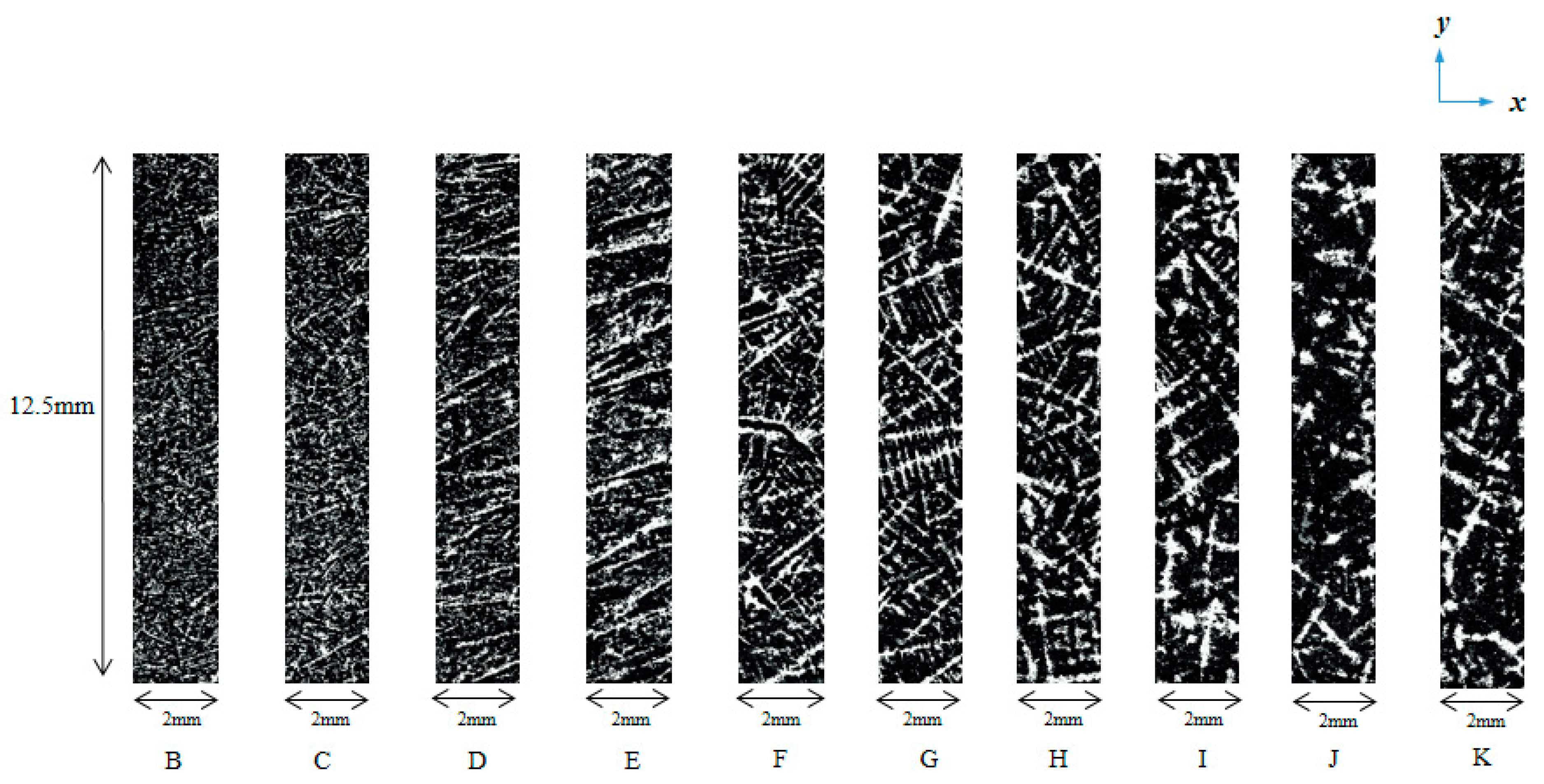
2.1. Sample Preparation

The main chemical composition (mass fraction, %) of GCr15 bearing steel is C1.02, Cr1.50, Mn0.30, Si0.25, and the rest is Fe. GCr15 bearing steel is a kind of classic advanced high-strength alloy that has been applied in many manufacturing aspects. The schematic of curved continuous casting machine is shown in Figure 1.

After solidifying, the sample of GCr15 steel was obtained by cutting along the transverse section of the bloom. Then, the sample surface was polished and smooth as a mirror. In order to get the $h_{es}^{}$, which is caused by different carbon contents, the commonly used hot pickling experiment with 50% hydrochloric acid–water solution (the bath temperature is 60–80 °C and the etching time is 25 min) [19,21] was carried out. The surface was cleaned at once by swiping in warm water and blow-dried quickly after removing it from the pickling solution. The sample etched casting macrostructures are shown in Figure 2a,c, which are mainly comprised of casting columnar and equiaxed dendritic grains (white part). The bloom casting processes are shown in

Table 1. Main continuous casting process parameters of GCr15 steel bloom.

Sample	Superheat, °C	Casting Speed, m/min	Specific Water Ratio, L/kg
1#	20	1.1	0.38
2#	35	1.1	0.38

; the only difference between 1# sample and 2# sample is the casting superheat, which is measured in the tundish. The superheat of 1# sample (20 °C) was lower than that of 2# sample (35 °C).

The $h_{es}^{}$ was measured by a 3D Measuring Laser Microscope produced by Olympus company (LEXT OLS4000, Tokyo, Japan). Due to the microscope limiting, the rectangular areas (12.5 mm × 220 mm) from the inner curve side to the outer curve side were first chosen to implement measuring, as shown in Figure 2b,d.

Taking the inner curve side as an example, line sweeping measurement was performed at 13 positions (A to M in Figure 3) from down to up, as shown by the vertical dashed arrow line in Figure 3.

The distances to the bloom edges at A–M were 1, 3, 5, 10, 20, 30, 40, 50, 60, 70, 80, 90 and 100 mm, respectively. Thus, as to each bloom, there were 26 positions of line sweeping for both inner curve and out curve sides. Because the microscope can measure a height every 0.25 μm, the total measuring points at a position (the length is 12.5 mm) were 50,001, which was enough for statistical calculation. The measurement in Figure 3 is for velocity magnitude calculation. For velocity direction, 1 mm long measuring was conducted at the left side and the right side of each position, as shown by the horizontal dashed arrow lines (α and β) from bloom edge toward center in Figure 4 where the vertical dashed arrow corresponds to the same arrow in Figure 3.

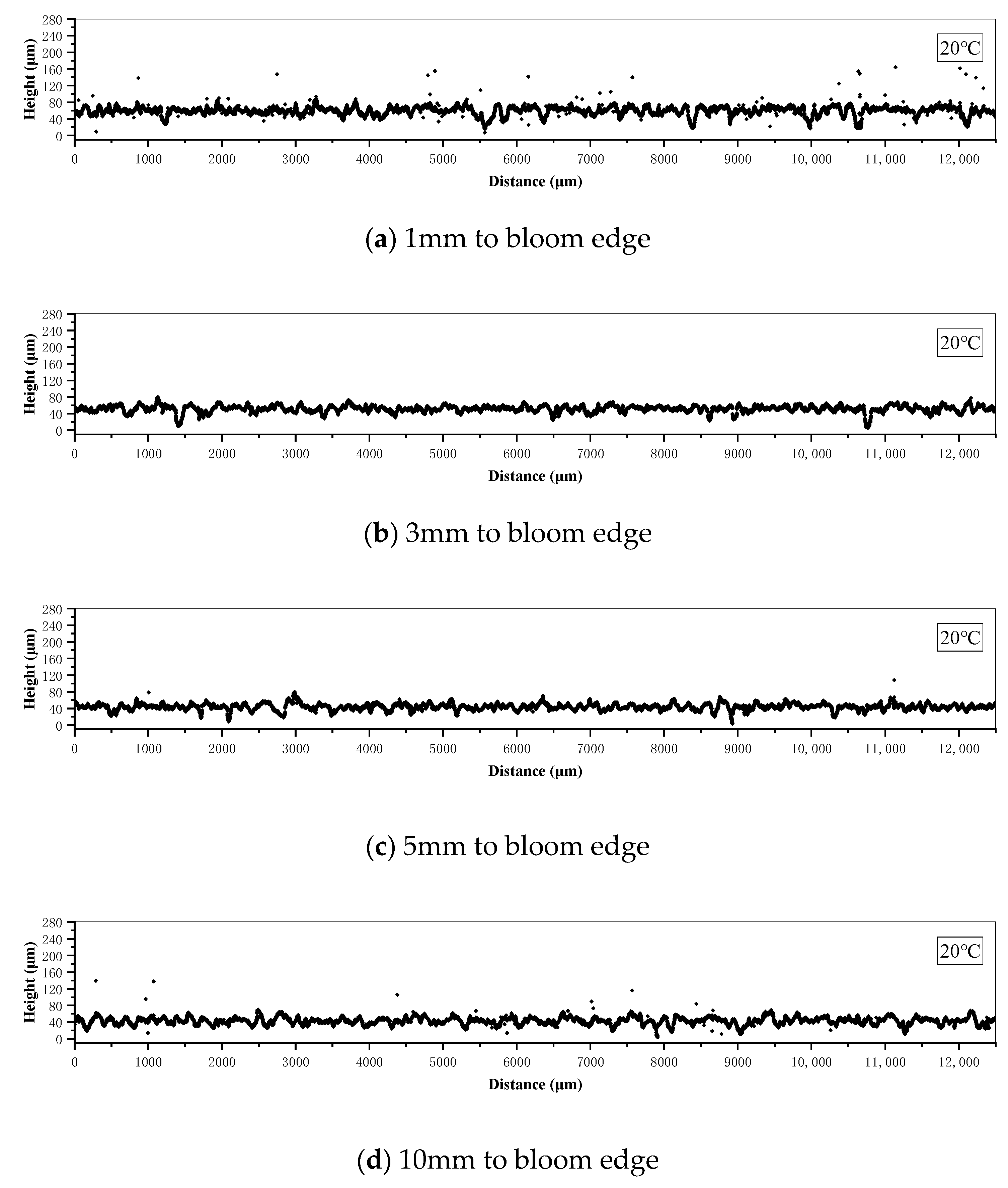
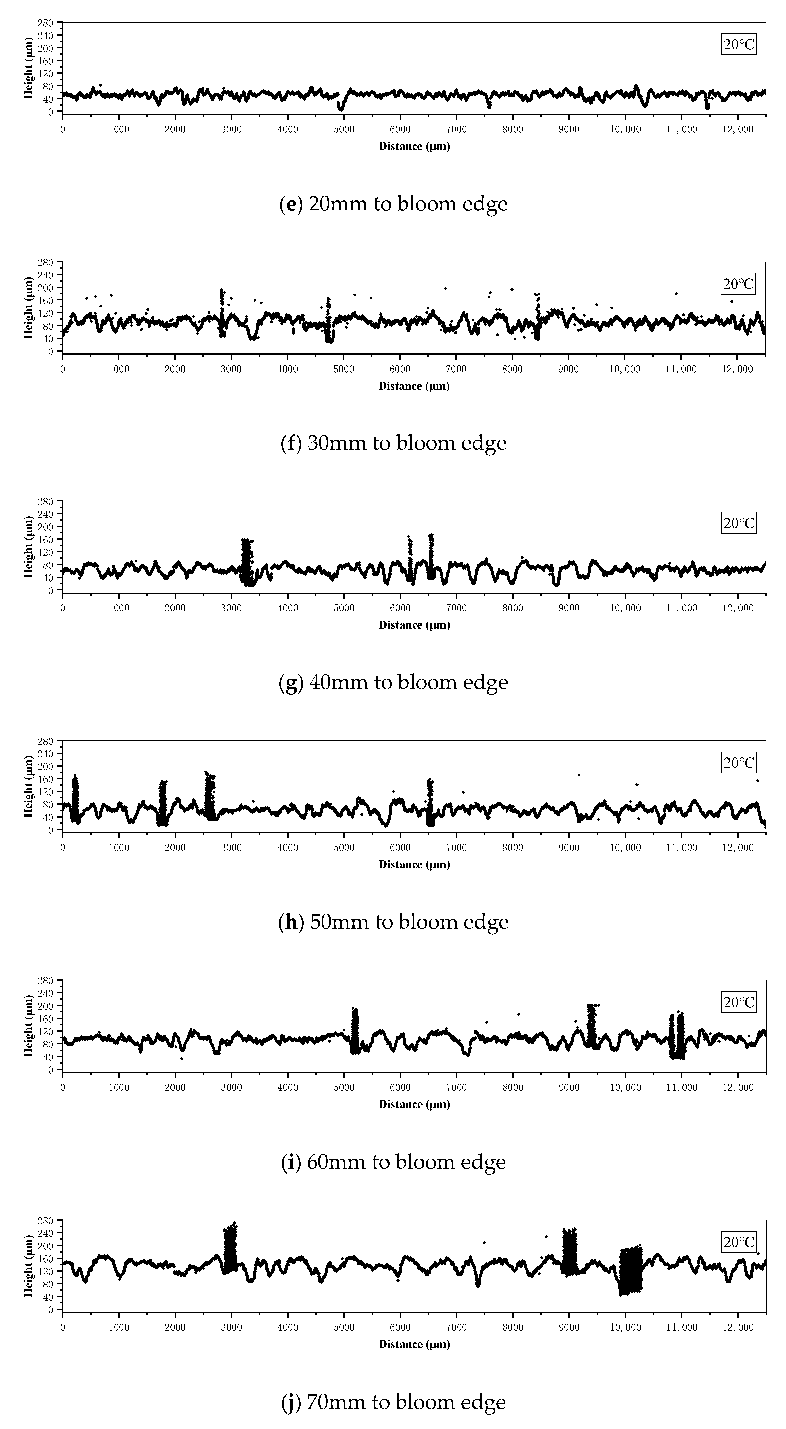
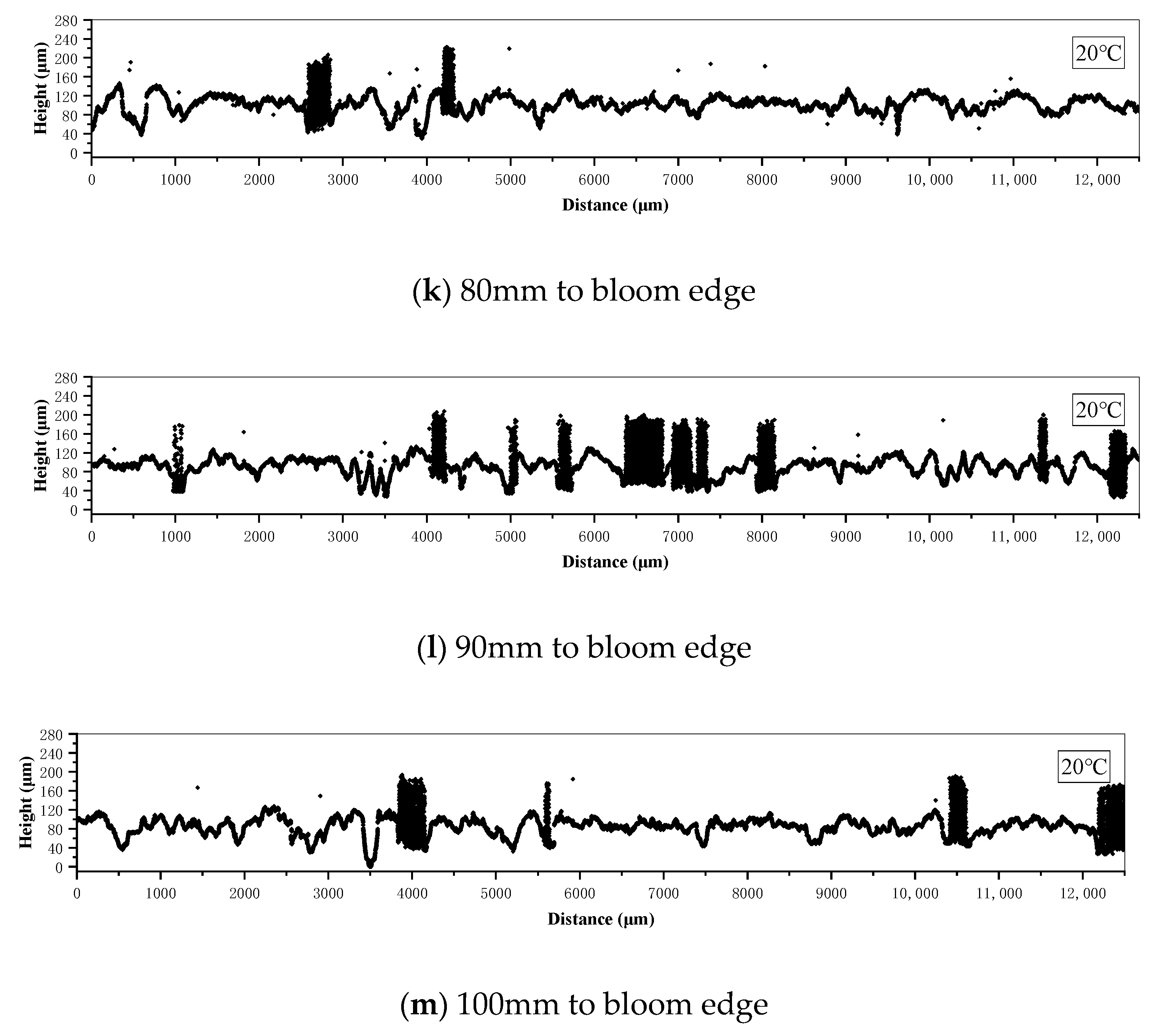
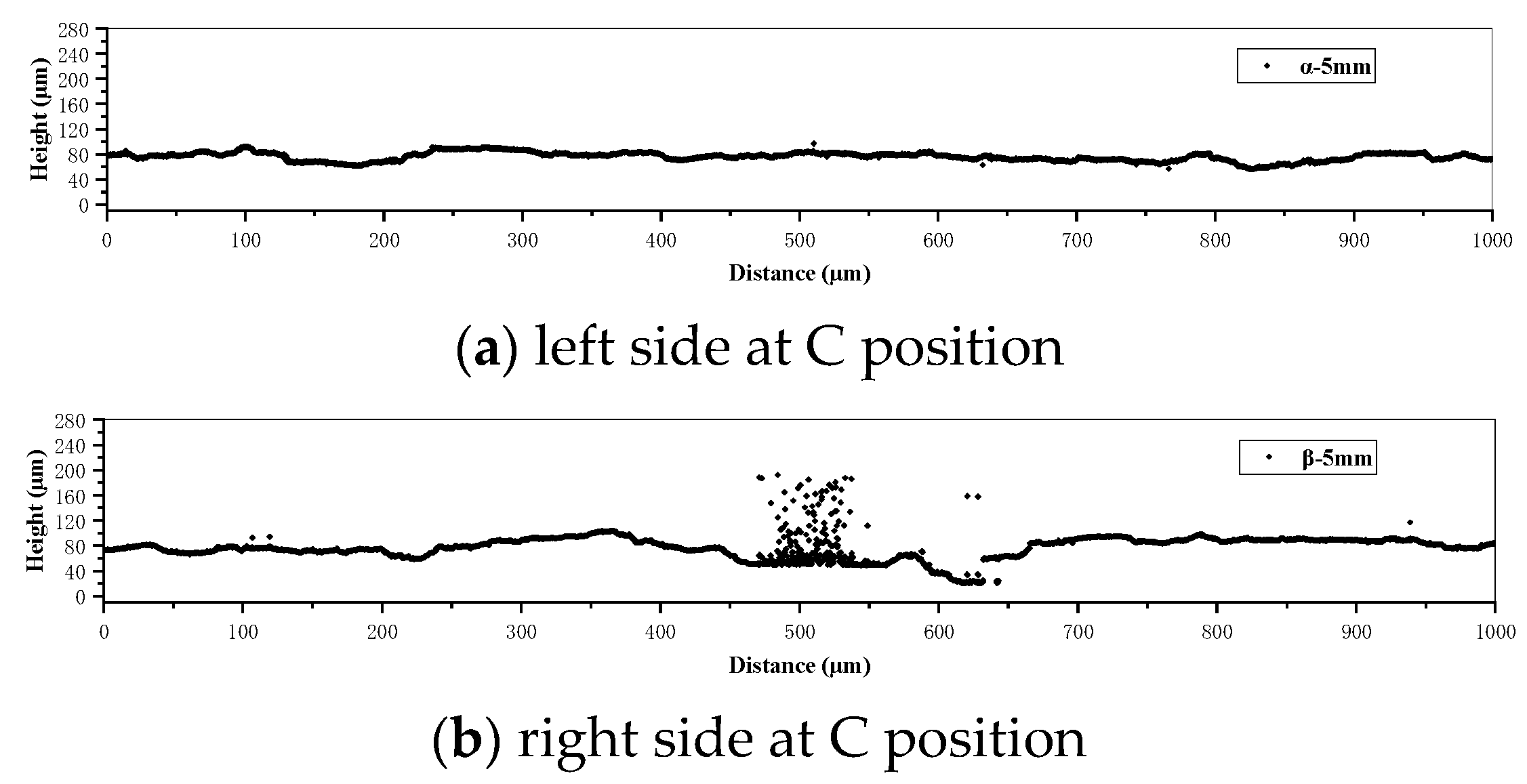
2.2. Etched Surface Height

After measuring, the surface heights at A position in the outer curve side under 35 °C superheat were obtained as shown in Figure 5a. In addition to the height fluctuation, we found that the heights decreased linearly with increasing the distance as a whole (marked schematically by the inclined arrow line in Figure 5a). In fact, this distinct whole decreasing trend could have been caused by the original uneven surface before hot pickling, and it is very difficult to remove completely with the existing polishing technology. In order to eliminate the unexpected influence of the original unevenness, the cutoff length λc = 2.5 mm was chosen to filter the original data on the basis of the surface roughness theory [24,25]. The corresponding filtered heights at A position are shown in Figure 5b, which is characteristic of the almost flat basic surface marked schematically by a horizontal arrow line. Therefore, all heights at different positions were filtered before model construction. For the bloom sample under 20 or 35 °C superheats, the inner curve side and the outer curve side all had 13 sets of data like Figure 5b. For example, the $h_{es}^{}$ of different positions in the inner curve side under 20 °C are shown in Figure 6.

Meanwhile, the $h_{es}^{}$ values for velocity direction were measured, as seen in Figure 4. Left side (α) and right side (β) $h_{es}^{}$ at only 10 positions (B, C, D, E, F, G, H, I, J, K) in the inner curve side under 20 °C were obtained because the bloom was too big to measure any points on the surface, and the time for keeping the etched surface un-oxidized was limited. As two examples, the heights of the left and right sides at B position and C position are shown in Figure 7 and Figure 8, respectively. We found in part that the difference between the left and right sides at C position was more obvious than that at B position.

3. Model Description

Figure 9a shows the macrostructure of the red rectangular area from Figure 4. The white part displays the dendrite grain morphology, and the black part displays the interdendritic area, which is characteristic of high element content. The horizontal dashed arrow corresponds to the vertical dashed arrow in Figure 3. Figure 9b is the etched surface height distribution along the horizontal dashed arrow in Figure 9a. Taking F position in the inner curve side under 20 °C as an example, by comparing Figure 9a with Figure 9b, we found that the heights in the dendrite centers always had a relative maximum value of height (e.g., (1), (2) and (5) points marked by the intersection between the red dashed line and horizontal dashed arrow), and the heights in the black interdendritic areas always had a relative minimum value of height (e.g., (3), (4) and (6) points marked by the intersection between the green dashed line and horizontal dashed arrow).

In addition, the heights may seem not to be larger or smaller when the point is closer to or farther from the grain center. This is because the surface macrostructure is photographed by a SELP1650 digital camera, which cannot display three-dimensional morphology (i.e., the height difference) and some dendrites are cut off by cross section. Notwithstanding, the above discussion indicates that there is some correlation between the etched surface height and segregating element content. Carbon is the element segregated most in GCr15 bearing steel solidification [17,19]. Therefore, based on the characteristics of $h_{es}^{}$ distribution, a quantitative correlation equation between $h_{es}^{}$ and the dimensionless quantity of carbon content is put forward firstly, given by Equation (1). $C_d^{}$ is the dimensionless quantity of carbon content. At a certain position, 50,001 effective carbon contents are rearranged in descending order. Then, if the 12.5 mm measuring line at each position is treated as a solidification unit for the reason that every point on a measuring line has almost the same solidifying condition, the rearranged contents can be displayed by liquid fraction as a horizontal axis from a statistical average angle, as shown in Figure 10.

That is to say, the highest $C_d^{}$ can be regarded the final solidifying point, and the lowest is the original solidifying point. The content in solidus increases when liquid fraction is decreasing.

$$C_d=\frac{(h_{es}^a-h_{es}^i)}{h_{es}^a}+1$$

(1)

where $C_d^{}$ is the dimensionless quantity of carbon content at a point. $h_{es}^i$ is the etched surface height at a point. $h_{es}^a$ is the average height of the etched surface at each position.

In order to analyze the interdendritic fluid flow of macrosegregation that mainly happens in the middle and late period, the period with 0 to 0.7 liquid fraction in Figure 10 will be the focus of research (e.g., Figure 11). According to the near-equilibrium solidification model (NESM) where no diffusion occurs in solids and finite diffusion occurs in liquids [7,26,27], it is assumed that the distribution in Figure 11 should be expressed well by Equation (3) at all positions. Equation (2) is obtained by using the Scheil equation form to effectively describe element distribution in the near-equilibrium solidification model [28,29].

As $C_d$ can be considered as solid content $C_S^{*}$ on the basis of Equation (1), Equation (3) can be obtained on the basis of Equation (2) and be used to fit the content distribution like that in Figure 10 using the Levenberg–Marquardt algorithm [30]. These fitting calculations were carried out using Microsoft Excel software.

$$C_S^{*}=k_E{C}_0{f}_L{}^{(k_E-1)}$$

(2)

where $C_S^{*}$ is the solute content at the solid phase of the solidifying interface. $k_E$ is the effective solute redistribution coefficient at the solidifying interface in the NESM. $C_0$ is the original solute content before solidification. $f_L$ is the liquid fraction.

$$C_d=\mu f_L{}^{\gamma }$$

(3)

where $\mu =k_E{C}_{d_0}$, $\gamma =k_E-1$, and $C_{d_o}$ is the original dimensional quantity of carbon content. By Equation (1), $C_{d_o}$ should be equal to 1 under ideal conditions and is the calculated result of $\delta /(\gamma +1)$.

The difference of the distribution characteristics between the 0 to 0.7 liquid fraction and the 0.7 to 1.0 liquid fraction may be attributed to rare interdendritic flow in the initial period with nucleation and original growth. In fact, it is not easy to obtain the whole element distribution of a dendrite grain, especially for the distribution in the final stage of solidification, because some more complicate reactions (e.g., eutectic reaction) will occur for multicomponent alloys such as steel. Moreover, only in the two-dimensional surface of the actual ingot, the morphology appearing in the surface may not be representative of the three-dimensional grains structure. Owing to the above reasons, 12.5 mm long is measured to obtain enough data, which is more than 10 times a dendrite’s width. Thus, even though the surface morphology information displays incompletely for the whole grain structures at some points, the statistically average features of a rearranged distribution of a great many heights could represent effectively the segregating element content distribution of the position by eliminating the deviation of original data as far as possible.

All fitted results at each positions are shown in

Table 2. Fitted and calculated results in the inner curve side under 20 °C ($\mu$, $\gamma$ are fitted coefficients in Equation (3), and $R^2$ is the corresponding determination coefficient. $k_E$ is the effective solute redistribution coefficient. $M_y$ is growth velocity magnitude in the solidification unit along the measuring line at each position. ${\delta }_{Ca}$ is the average thickness of the concentration boundary layer).

Distance to Bloom Edge, mm	$\mathit{\mu }$	$\mathit{\gamma }$	${\mathit{R}}^2$	${\mathit{k}}_{\mathit{E}}$	${\mathit{M}}_{\mathit{y}}, \mathbf{mm}/\mathbf{s}$	${\mathit{\delta }}_{\mathit{C}\mathit{a}}, \mathbf{mm}$	$\mathit{\mu }/(\mathit{\gamma }+1)$
1	0.8903	−0.132	0.9713	0.868	0.2125	0.0960	1.03
3	0.9089	−0.115	0.9849	0.885	0.1661	0.1276	1.03
5	0.9224	−0.114	0.9695	0.886	0.1197	0.1775	1.04
10	0.9158	−0.128	0.9338	0.872	0.0782	0.2631	1.05
20	0.8841	−0.142	0.9772	0.858	0.0457	0.4371	1.03
30	0.9055	−0.124	0.9634	0.876	0.0310	0.6707	1.03
40	0.8784	−0.166	0.9158	0.834	0.0227	0.8413	1.05
50	0.8824	−0.169	0.9072	0.831	0.0189	1.0027	1.06
60	0.9105	−0.120	0.9429	0.880	0.0170	1.2317	1.03
70	0.9243	−0.104	0.9496	0.896	0.0156	1.3922	1.03
80	0.9154	−0.120	0.9548	0.880	0.0146	1.4312	1.04
90	0.9069	−0.143	0.9189	0.857	0.0140	1.4277	1.06
100	0.8835	−0.157	0.9558	0.843	0.0136	1.4298	1.05

,

Table 3. Fitted and calculated results in the outer curve side under 20 °C ($\mu$, $\gamma$ are fitted coefficients in Equation (3), and $R^2$ is the corresponding determination coefficient. $k_E$ is the effective solute redistribution coefficient. $M_y$ is growth velocity magnitude in the solidification unit along the measuring line at each position. ${\delta }_{Ca}$ is the average thickness of the concentration boundary layer).

Distance to Bloom Edge, mm	$\mathit{\mu }$	$\mathit{\gamma }$	${\mathit{R}}^2$	${\mathit{k}}_{\mathit{E}}$	${\mathit{M}}_{\mathit{y}}, \mathbf{mm}/\mathbf{s}$	${\mathit{\delta }}_{\mathit{C}\mathit{a}}, \mathbf{mm}$	$\mathit{\mu }/(\mathit{\gamma }+1)$
1	0.9226	−0.109	0.9396	0.891	0.2125	0.1011	1.04
3	0.9107	−0.123	0.9526	0.877	0.1661	0.1253	1.04
5	0.934	−0.132	0.9738	0.868	0.1197	0.1705	1.08
10	0.9295	−0.103	0.9777	0.897	0.0782	0.2788	1.04
20	0.8968	−0.129	0.9872	0.871	0.0457	0.4492	1.03
30	0.8845	−0.157	0.9548	0.843	0.0310	0.6264	1.05
40	0.8764	−0.168	0.9116	0.832	0.0227	0.8381	1.05
50	0.9027	−0.141	0.9112	0.859	0.0189	1.0594	1.05
60	0.8711	−0.185	0.9004	0.815	0.0170	1.0819	1.07
70	0.9027	−0.132	0.9279	0.868	0.0156	1.3058	1.04
80	0.9341	−0.117	0.8953	0.883	0.0146	1.4410	1.06
90	0.9126	−0.145	0.8871	0.855	0.0140	1.4219	1.07
100	0.9257	−0.114	0.906	0.886	0.0136	1.5661	1.04

,

Table 4. Fitted and calculated results in the inner curve side under 35 °C ($\mu$, $\gamma$ are fitted coefficients in Equation (3), and $R^2$ is the corresponding determination coefficient. $k_E$ is the effective solute redistribution coefficient. $M_y$ is growth velocity magnitude in the solidification unit along the measuring line at each position. ${\delta }_{Ca}$ is the average thickness of the concentration boundary layer).

Distance to Bloom Edge, mm	$\mathit{\mu }$	$\mathit{\gamma }$	${\mathit{R}}^2$	${\mathit{k}}_{\mathit{E}}$	${\mathit{M}}_{\mathit{y}}, \mathbf{mm}/\mathbf{s}$	${\mathit{\delta }}_{\mathit{C}\mathit{a}}, \mathbf{mm}$	$\mathit{\mu }/(\mathit{\gamma }+1)$
1	0.9336	−0.076	0.9615	0.924	0.1928	0.1218	1.01
3	0.9188	−0.105	0.9859	0.895	0.1496	0.1451	1.03
5	0.9283	−0.089	0.9439	0.911	0.1064	0.2125	1.02
10	0.9161	−0.113	0.9702	0.887	0.0728	0.2926	1.03
20	0.8988	−0.130	0.9793	0.870	0.0435	0.4712	1.03
30	0.9029	−0.125	0.9706	0.875	0.0296	0.6991	1.03
40	0.9179	−0.108	0.9771	0.892	0.0224	0.9613	1.03
50	0.8972	−0.128	0.9558	0.872	0.0191	1.0751	1.03
60	0.8834	−0.154	0.9062	0.846	0.0172	1.1343	1.04
70	0.8944	−0.120	0.9143	0.880	0.0158	1.3273	1.02
80	0.9042	−0.112	0.9840	0.888	0.0148	1.4442	1.02
90	0.8897	−0.151	0.9554	0.849	0.0141	1.3918	1.05
100	0.9239	−0.117	0.9517	0.883	0.0137	1.5435	1.05

and

Table 5. Fitted and calculated results in the outer curve side under 35 °C ($\mu$, $\gamma$ are fitted coefficients in Equation (3), and $R^2$ is the corresponding determination coefficient. $k_E$ is the effective solute redistribution coefficient. $M_y$ is growth velocity magnitude in the solidification unit along the measuring line at each position. ${\delta }_{Ca}$ is the average thickness of the concentration boundary layer).

Distance to Bloom Edge, mm	$\mathit{\mu }$	$\mathit{\gamma }$	${\mathit{R}}^2$	${\mathit{k}}_{\mathit{E}}$	${\mathit{M}}_{\mathit{y}}, \mathbf{mm}/\mathbf{s}$	${\mathit{\delta }}_{\mathit{C}\mathit{a}}, \mathbf{mm}$	$\mathit{\mu }/(\mathit{\gamma }+1)$
1	0.9451	−0.085	0.9681	0.915	0.1928	0.1186	1.03
3	0.9232	−0.096	0.9809	0.904	0.1496	0.1484	1.02
5	0.9387	−0.085	0.9631	0.915	0.1064	0.2149	1.03
10	0.9162	−0.103	0.9811	0.897	0.0728	0.2997	1.02
20	0.9119	−0.117	0.9832	0.883	0.0435	0.4850	1.03
30	0.9040	−0.122	0.9706	0.878	0.0296	0.7037	1.03
40	0.9182	−0.111	0.9713	0.889	0.0224	0.9545	1.03
50	0.9002	−0.128	0.972	0.872	0.0191	1.0751	1.03
60	0.8807	−0.149	0.9639	0.851	0.0172	1.1456	1.03
70	0.9171	−0.137	0.9316	0.863	0.0158	1.2791	1.06
80	0.9148	−0.117	0.9545	0.883	0.0148	1.4275	1.04
90	0.9337	−0.088	0.9864	0.912	0.0141	1.6087	1.02
100	0.8952	−0.136	0.9415	0.864	0.0137	1.4805	1.04

. The determination coefficient $R^2$ is calculated as Equation (4) [30]. When $R^2$ is closer to 1, the fitted formula can express the original data more effectively. Because all R² are almost bigger than 0.9 (more than half of them bigger than 0.95), it means that Equation (3) is a good formula to quantitatively describe the content distribution with 0 to 0.7 liquid fraction at all positions.

$$R^2=\frac{{\displaystyle \sum _{i=1}^n{({\widehat{y}}_i-\overline{y})}^2}}{{\displaystyle \sum _{i=1}^n{(y_i-\overline{y})}^2}}$$

(4)

where $y_i$ is the original value. $\overline{y}$ is the average of the original value. ${\widehat{y}}_i$ is the corresponding regression value.

Based on fitted parameters and Equation (3), $k_E$ is obtained on the basis of $\gamma$ value. Meanwhile, the fitted $C_{d_o}$ is almost equal to 1 in Table 2, Table 3, Table 4 and Table 5, which indicates that Equation (2) and the NESM are suitable to describe the distribution because the ideal $C_{d_o}$ is equal to 1, further indicating that the above method is suitable to calculate the $k_E$ value.

Meanwhile, according to the theory suggested by Burton and his co-workers [27,31], $k_E$ at the solidifying interface in the NESM can also be calculated theoretically by Equation (5). Then, the average thickness of concentration boundary layer ${\delta }_{Ca}$ can be obtained by Equation (6).

$$k_E=\frac{k_0}{k_0+(1-k_0)e^{-\frac{M_y}{D}{\delta }_{Ca}^{}}}.$$

(5)

Then,

$${\delta }_{Ca}=-\frac{D}{M_y}\ln \left[\frac{k_0-k_0{k}_E}{k_E(1-k_0)}\right]$$

(6)

where ${\delta }_{Ca}$ is the average thickness of the concentration boundary layer. $D$ is the mass diffusivity of the carbon element, 0.005 m²/s [32]. $k_0$ is the ideal solute redistribution coefficient and is chosen as 0.1 for the carbon element [33]. $M_y$ is the corresponding growth velocity magnitude in the solidification unit along the measuring line at each position, which can be calculated by Equation (7).

$$M_y=L/\left(\frac{T_l-T_s}{R}\right)$$

(7)

where $L$ is the measuring length at each position, 12.5 mm. $T_l$ and $T_s$ are the liquidus temperature (1466 °C) and solidus temperature (1328 °C) of GCr15. $R$ is the cooling rate (°C/s), which is calculated by thermal simulation of the finite element model, and the governing equations are Equations (8) and (9) [33]. Axial heat conduction in the casting direction was ignored.

$$\frac{\partial T}{\partial t}=\frac{\lambda }{\rho S_h}\left(\frac{{\partial }^{2}T}{\partial x^2}+\frac{{\partial }^{2}T}{\partial y^2}\right)$$

(8)

where $T$ is the temperature. $t$ is time. $\lambda$ is the thermal conductivity. $\rho$ is the density. $S_h$ is the specific heat. The evolution of the latent heat during the solidification was incorporated into the calculation by using the effective specific heat method, as shown in Equation (9) [34].

$$S_h{}^{\prime }=S_h-H_L\left(\frac{d{f}_s}{dT}\right)$$

(9)

where $S_h{}^{\prime }$ is the effective specific heat. $H_L$ is the latent heat and $f_s$ is the solid fraction.

Combining measured $k_E$ in Table 2, Table 3, Table 4 and Table 5 with the aforementioned equations, ${\delta }_{Ca}$ can be calculated as shown in Table 2, Table 3, Table 4 and Table 5. Regardless of whether it is laminar flow or turbulent flow, there is a boundary layer during the initial stage that can be assumed to feature laminar flow characteristics, especially in the limited length on a flat plate [35]. Thus, in this research, the interdendritic flow on dendritic grain structure in each position can be considered as the flat plate flow model because there is only enough space to flow during the solidifying process. According to the dimensionless equation in the transport phenomena of the boundary layer theory [32,35], the average thickness of the velocity boundary layer ${\delta }_{Va}$ can be calculated by Equation (10) after getting ${\delta }_{Ca}$.

$$\frac{{\delta }_{Va}}{{\delta }_{Ca}}=S{c}^{1/3}={(\frac{\mu }{\rho D})}^{1/3}$$

(10)

where $Sc$ is Schmidt number. $\mu$ is the dynamic viscosity, 0.0067 Pa·s, and $D$ is the mass diffusivity of the carbon element, 0.005 m²/s, and $\rho$ is the density, 7600 kg/m³ [32].

Based on the boundary layer theory [34,35], the change of thickness of the velocity boundary layer ${\delta }_V$ with velocity $V$ and flow length $\varphi$ can be described by Equation (11), the average thickness ${\delta }_{Va}$ in $\varphi$ long zone can be expressed by Equation (12).

$${\delta }_V=4.64{\left(\frac{\mu \varphi }{\rho V}\right)}^{1/2}.$$

(11)

Then,

$${\delta }_{Va}=\frac{{\displaystyle {\int }_0^{\varphi }4.64{\left(\frac{\mu \varphi }{\rho V_{{\delta }_{Va}}}\right)}^{1/2}}d\varphi }{\varphi }=4.64\times \frac{2}{3}\times {\left(\frac{\mu }{\rho V_{{\delta }_{Va}}}\right)}^{1/2}\times {\varphi }^{1/2}.$$

(12)

From Equation (12), the equivalent flow velocity $V_{{\delta }_{Va}}$ can be calculated by Equation (13):

$$V_{{\delta }_{Va}}=\frac{{4.64}^2\times {\left(\frac{2}{3}\right)}^2\times \frac{\mu }{\rho }\times \varphi }{{\delta }_{Va}}$$

(13)

where ${\delta }_{Va}$ is obtained by Equation (10). $\varphi$ is chosen as 1 mm based on the measuring size.

Meanwhile, there is also the original thickness of the concentration boundary layer without fluid flow, which can be calculated by Equation (14), only considering molecular diffusion [36].

$$C_L^{}=C_0[1+\frac{(1-k_0)}{k_0}{e}^{-\frac{M_y}{D}{\delta }_{C{a}_o}}].$$

(14)

Based on Equation (14), when $C_L^{}/C_0$ = 1.01, the original thickness of the concentration boundary layer ${\delta }_{C{a}_0}$ can be obtained by Equation (15). Then the original thickness of the velocity boundary layer ${\delta }_{V{a}_0}$ can also be calculated by Equation (10).

$${\delta }_{C{a}_o}=-\frac{D}{M_y}\ln (\frac{0.01k_0}{(1-k_0}).$$

(15)

On the basis of ${\delta }_{C{a}_o}$ and ${\delta }_{Ca}$, ${\delta }_{V{a}_o}$ and ${\delta }_{Va}$ can be obtained. Then, the corresponding velocity can be calculated. Finally, the difference between $V_{{\delta }_{Va}}$ and $V_{{\delta }_{V{a}_o}}$ is the magnitude of interdendritic fluid flow velocity $V_{iff}$, as shown in Equation (16). The corresponding flowchart is also shown in Figure 12.

$$V_{iff}=V_{{\delta }_{Va}}-V_{{\delta }_{V{a}_o}}$$

(16)

Following is the calculation method for the direction of interdendritic flow velocity with respect to the above $V_{iff}$. In Figure 4, the measuring heights of 1 mm length α and β should have the same features if there is no fluid flow because the left and right sides are almost under the same solidifying conditions for their limited distance. Then the standard deviation $S_d$ as shown in Equation (17) [30], is firstly introduced to measure the fluctuation extent of left or right side heights.

$$S_d=\sqrt{\frac{{\displaystyle \sum _{i=1}^n{(h_{es}^i-h_{es}^a)}^2}}{n-1}}$$

(17)

where $h_{es}^i$ is the etched surface height at $i$ point. $h_{es}^a$ is the average value of the etched surface height. $n$ is the number of the point.

$$E_{VD}=S_d^L-S_d^R$$

(18)

where $E_{VD}$ is the difference value. $S_d^L$ is the standard deviation of the left side, and $S_d^R$ is the standard deviation of the right side.

As shown in Equation (18), the standard deviation difference between left side and right side is introduced to measure the velocity direction. As a matter of fact, because interdendritic fluid flow can induce more stochastic solidification behavior [7,36], it was assumed in this research that the main fluid flow direction is from right side to left side if $E_{VD}$ is positive, and the main fluid flow direction is from left side to right side if $E_{VD}$ is negative. The absolute value of $E_{VD}$ should indicate the extent along the growth direction. Actually, interdendritic fluid flow exists in three-dimensional space, and the calculated velocity magnitude above is also a three-dimensional value. Considering the surface from the inner curve side to outer curve side as x-positive axis, the grain growth direction from bloom left edge to center as y-positive axis, and the casting direction as z-positive axis, as shown in Figure 13, only the velocity direction component $\theta$ on xz plane can be obtained because only left and right side heights on the cross section are measured here.

As to the degree $\theta$, its value can be calculated by Equation (19), assuming the position with the largest absolute value of difference has the same or symmetric degree (0° or 180°) to grain growth direction. The degree calculation flowchart is also shown in Figure 14.

$$\theta =\arccos (\frac{E_{VD}}{-\left|E_{VD}^{\max }\right|})/\pi \times 180°$$

(19)

where $\theta$ is the degree of fluid flow direction on the xz plane with respect to the x-positive axis in Figure 13, and arccos is the anticosine sign. $E_{VD}^{\max }$ is the standard deviation difference, which has the maximum absolute value among all points. The denominator in Equation (19) is the negative value of the absolute of $E_{VD}^{\max }$.

4. Results and Discussion

Based the above model, the magnitude and direction of velocity of interdendritic fluid during metal solidifying can be calculated. We will discuss these results under different conditions in this section.

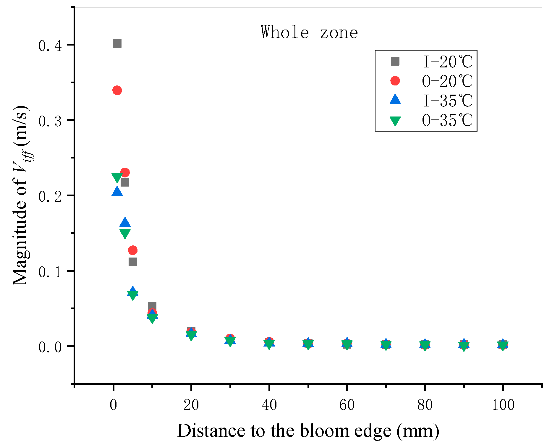
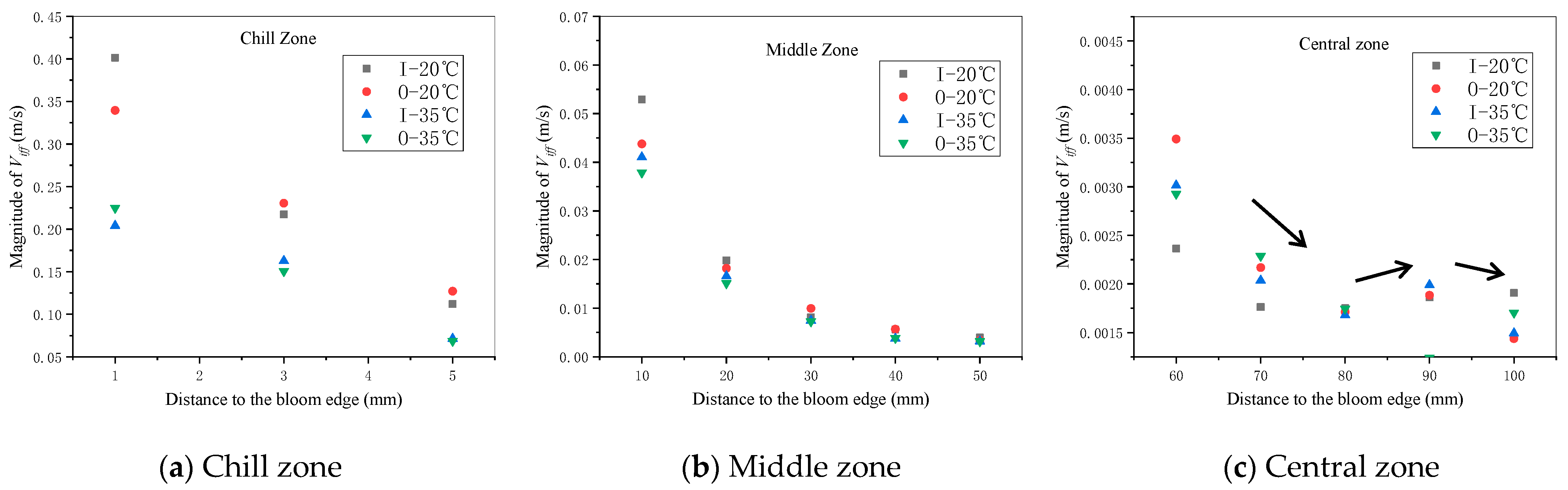
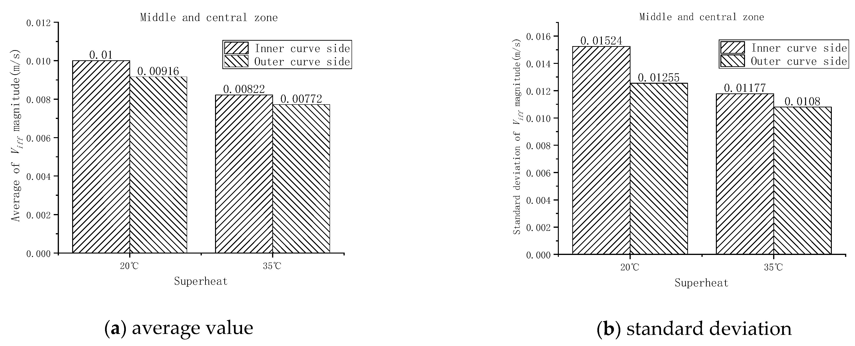
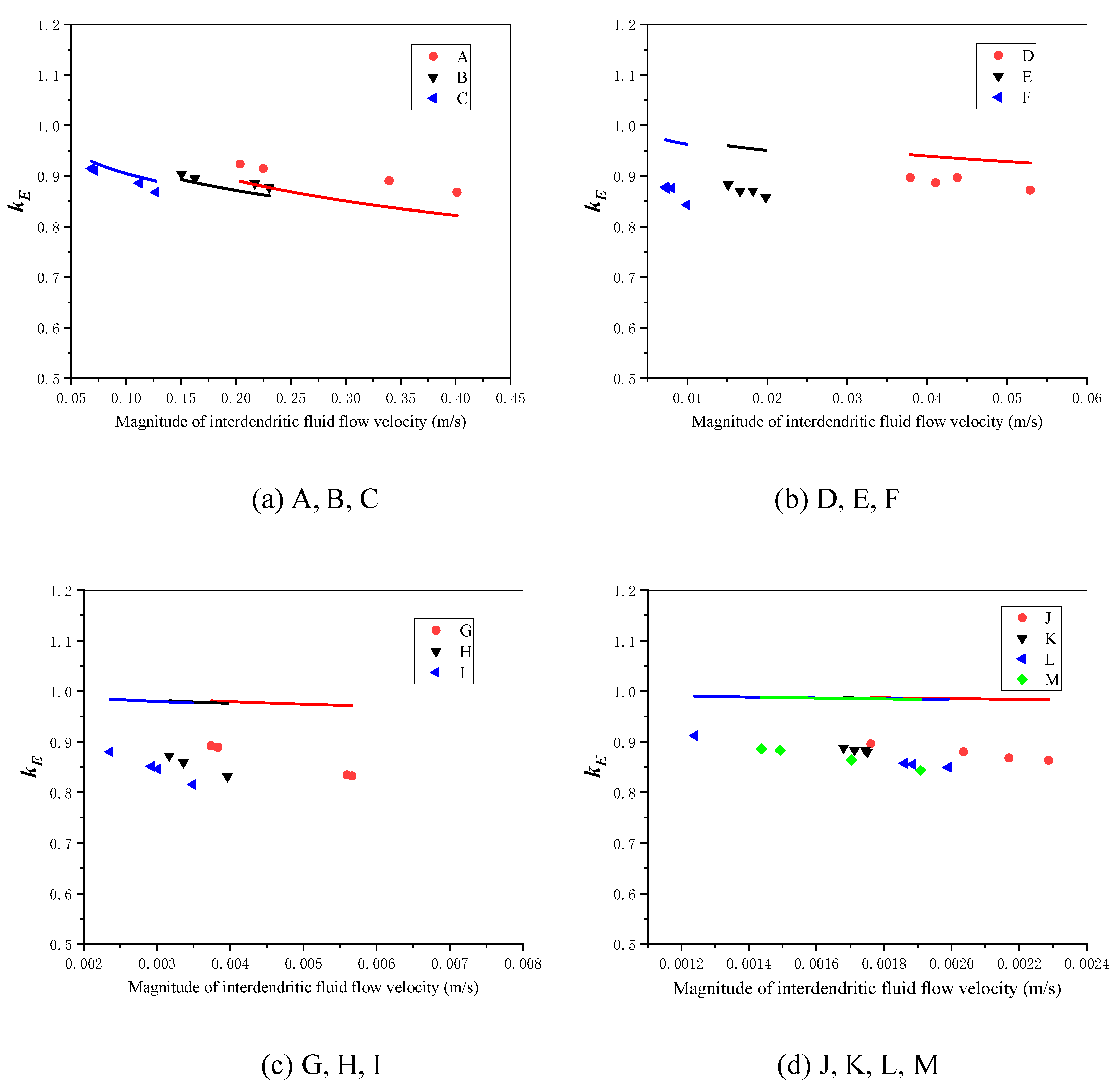
4.1. Magnitude of Interdendritic Fluid Flow Velocity

The $V_{iff}$ magnitudes at different positions shown in Figure 3 in inner and outer curve sides under different superheats (20 and 35 °C) are shown in

Table 6. Magnitude of interdendritic liquid flow velocity $V_{iff}$ in inner and outer curve sides under 20 and 35 °C.

Distance to Bloom Edge, mm	$\mathbf{Magnitude} \mathbf{of} \mathbf{Interdendritic} \mathbf{Liquid} \mathbf{Flow} \mathbf{Velocity} {\mathit{V}}_{\mathit{i}\mathit{f}\mathit{f}}, \mathbf{m}/\mathbf{s}$
	20 °C		35 °C
	Inner Curve Side	Outer Curve Side	Inner Curve Side	Outer Curve Side
1	0.40143	0.33952	0.20392	0.22494
3	0.21726	0.23041	0.16279	0.15060
5	0.11190	0.12724	0.07137	0.06856
10	0.05290	0.04377	0.04105	0.03787
20	0.01981	0.01819	0.01658	0.01511
30	0.00806	0.00994	0.00744	0.00728
40	0.00560	0.00566	0.00374	0.00383
50	0.00396	0.00336	0.00317	0.00317
60	0.00236	0.00349	0.00301	0.00293
70	0.00176	0.00217	0.00204	0.00229
80	0.00175	0.00171	0.00168	0.00175
90	0.00186	0.00188	0.00199	0.00124
100	0.00191	0.00144	0.00149	0.00170

and Figure 15. We found that the magnitude decreased from the bloom edge to center as a whole. The high velocity magnitude near bloom edge could be attributed to the high flow velocity when the fluid moved from tundish to mold. Meanwhile, there was also electromagnetic stirring in the initial solidification in the mold.

Notwithstanding, in order to compare more clearly, each side was divided into three zones, i.e., chill zone, middle zone, and central zone in Figure 16. The chill zone contained three positions whose distances to the edge were 1, 3, and 5 mm, respectively. The middle zone contained five positions whose distances to the edge were 10, 20, 30, 40, and 50 mm, respectively. The central zone contained five positions whose distances to the edge were 60, 70, 80, 90, and 100 mm, respectively. Then we found that, a little different from the other zones, the velocity magnitude in the central zone decreased firstly, then showed an increasing trend and decreased again finally, as shown by arrow line in Figure 16c. This phenomenon was in correspondence with the extent of point and centerline segregation morphology of the central zone in Figure 2. The increasing trend could be attributed to the suction force to compensate the centerline porosity, i.e., the V segregation formation in continuous casting [6,7,37]. The reason for decreasing again could be M position being too close to the bloom center where solidifying completes quickly.

There was no apparent difference between different sides, but the corresponding average value displayed some regularity, if only for the middle and central zones. As shown in Figure 17a, not only under low superheat, but also under high superheat, both of the velocity magnitudes in the inner curve sides had a greater value than those in the outer curve sides. Meanwhile, as to the standard deviation calculated by Equation (16) in Figure 17b, the values in the inner curve side also had a greater value than those in the outer curve side. These phenomena indicated that there was more active interdendritic fluid flow in the inner curve side by comparison with the outer curve side, which corresponded with the gravity features of the curved segment of the continuous casting machine in Figure 1. However, as to the chill zone, as shown in Figure 18, there was no same trend under different superheats, and the extent of changing proportion was relatively minor. This is because the chill zone almost solidified completely in the mold instead of the curved segment. Meanwhile, Figure 19a,b display related average value and standard deviation, respectively. We found that the velocity magnitude and related fluctuation were higher under 20 °C.

Figure 20a,b reveal the secondary arm spacing (SDAS) at different locations and corresponding average values and standard deviations. SDASs were obtained by calculating the average value of 10 typical dendrite grains (the clear dendrite grains in the main area) in a 10 mm × 10 mm area at different positions. We found that the SDAS under 35 °C was higher because the bloom needed more time to solidify. According to Darcy’s law in Equation (20) [38], besides the SDAS, which positively influences the permeability, the velocity magnitude is also determined by the pressure gradient $\Delta P/L$ in the mushy zone.

$$V_{iff}=-\frac{K}{\epsilon \mu }\frac{\Delta P}{L}$$

(20)

where $K$ is the permeability. $\epsilon$ is the volume fraction of interdendritic liquid. $\mu$ is the viscosity. $\Delta P$ is the pressure loss and $L$ is the related distance.

Thus, the pressure magnitude should be greater under lower superheat, which has a narrower mushy zone owing to a shorter liquid core length in continuous casting bloom. Meanwhile, there was a positive relationship between the fluctuation of velocity magnitude and SDAS standard deviation, i.e., SDAS showed more fluctuant under 20 °C. Therefore, it was indicated that although the SDAS magnitude was mainly determined by the cooling rate, the fluctuation extent of SDAS was more relevant to interdendritic fluid flow by changing solute and thermal distribution, breaking dendrite, etc.

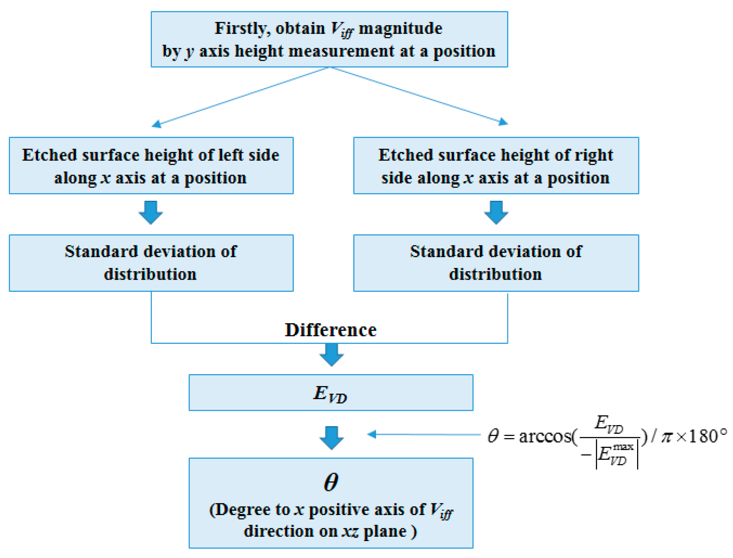
4.2. Direction of Interdendritic Fluid Flow Velocity

The differences of standard deviation between left side height and right side height $E_{VD}$ at different positions are shown in Figure 21. G position has the maximum absolute value of $E_{VD}$ among all points.

Because the grain growth direction was from the edge to the center, which is the more negative, the fluid flow was closer to the grain grow direction based on the above model. In Figure 22, the degree $\theta$ of fluid flow direction on the xz plane, as shown in Figure 13, and Equation (19) were obtained on the basis of assuming the position with the largest negative value of difference in Figure 21 (G position) had the same degree to grain growth direction, i.e., the degree was zero.

Because interdendritic fluid flow exists in three-dimensional space and the calculated velocity magnitude above is also a three-dimensional value, in order to compare them equally, the effective ratio between interdendritic flow velocity and growth velocity $(V_{iff}/M_x)e$ was calculated as Equation (21) which can contain the influence of velocity direction.

$${(\frac{V_{iff}}{M_x})}_e=\frac{V_{iff}\times \cos (\theta )}{M_x}$$

(21)

where $M_x$ is the growth velocity whose direction is from the bloom edge toward bloom center, and the magnitude is equal to 2000 mm/R, R is the cooling rate (°C/s), which was calculated by the above thermal simulation of finite element model. $\theta$ is the degree of fluid flow direction on the xz plane with respect to the x-positive axis.

At the same time, the segregation area ratios at different positions were calculated by Equation (22) for the reason that it can reflect in part the related two-dimensional segregation extent caused by interdendritic fluid flow [21,39]. With the SELP1650 digital camera produced by Sony Corporation (Tokyo, Japan), the macrostructures whose locations are marked by a red rectangle in Figure 4 at 10 positions (B, C, D, E, F, G, H, I, J, K) in the inner curve side under 20 °C were obtained as shown in Figure 23. These macrostructures were used to calculate the corresponding segregation area ratios that display in Figure 24. B, C, D, J, and K mainly contained equiaxed grains, but E, F, G, H, and I mainly contained columnar grains.

$$R_{seg}=\frac{A_{seg}}{A_t}\times 100\%$$

(22)

where, $R_{seg}$ is the segregation area ratio, %, $A_t$ is the total analyzing area, 25 mm², $A_{seg}$ is the area of segregation points (black part), mm².

Figure 25 shows the relationship between $R_{seg}$ and $(V_{iff}/M_x)e$. Firstly, the whole points do not display an apparent trend. However, if only analyzing the equiaxed grain positions (i.e., B, C, D, J, and K, which are marked by the dashed line.), we found that there was a positive correlation between $R_{seg}$ and $(V_{iff}/M_x)e$ which corresponded to the macrosegregation formation theory proposed by Fleimings and co-workers [4,5,6]. As to the columnar grain positions marked by the dot-dash line, they also show a minor increasing trend if excluding E position marked by the full line. This may be because, compared with the dendritic columnar grain, the morphology in E position is a cell columnar grain, which grows under a higher temperature gradient. Meanwhile, the non-apparent increasing trend in the columnar grain zone may be attributed to its deviation from the assumption of the same solidifying condition for left side and right side at a certain position in the columnar grain zone of approximate directional solidification.

5. Model Verification Discussion and Further Work

From the aforementioned research, by establishing the model, the magnitude and direction of velocity were obtained. As for the verification of the model, the following results should first be provided: (1) The $\delta /(\gamma +1)$ values are almost equal to 1 in Table 2, Table 3, Table 4 and Table 5, which indicates that the above method is suitable to calculate $k_E$. (2) The comparison results of velocity magnitudes of different sides and under different superheats can be explained by continuous casting features and solidification theory. (3) There is a positive correlation between segregation area ratio and the effective ratio between interdendritic flow velocity and growth velocity, especially in the equiaxed grain zone.

Meanwhile, Takahashi et al. studied the relationship between interdendritic flow velocity and $k_E$ using a complex hot model experimental of steel ingot [40]. The fitted empirical formula is shown as Equation (23) [37,40]. By this equation, the $k_E$ is obtained on the basis of the calculated interdendritic flow velocity in this research. Figure 26 shows the empirical $k_E$ by Equation (23) and the measured $k_E$ in Table 2, Table 3 and Table 4 by the new approach.

The growth velocity at the same distance to the bloom edge was considered as the approximate average value of different superheats. By comparing $k_E$ in Figure 26, we found that the measured value and the empirical value had the same change trend with increasing interdendritic flow velocity, and the values were very close, especially in high flow velocity (i.e., Figure 26a). Meanwhile, the differences between the measured value and the empirical value were more distinct when the velocity was decreasing. The reason for this could be that the empirical formula Equation (23) was obtained on the basis of experimental high flow velocity. Additionally, the above velocity magnitude in Table 6 was from 0.001 to 1 m/s, which was approximately half of pure fluid velocity in some other simulated works by rough contrast [7,41,42,43]. In all, from the aforementioned discussion, what can be concluded is that the established method is available to obtain the magnitude and direction of interdendritic flow velocity.

$$k_E=1-1.33\times {10}^{-4}\times (1-k_0)\times (1-Sh)\times V_{iff}/M_y$$

(23)

where,

$$Sh=(V_{iff}/M_y)/(7500+V_{iff}/M_y).$$

This work provides a feasible method to obtain simultaneously the magnitude and the direction of $V_{iff}$ for two or three-dimensional multiscale velocity distribution by adjusting measuring length and numbers. Meanwhile, it should be noted that the calculated velocity in this paper is only a two-dimensional value, and it will need more related heights to calculate the whole three-dimensional velocity. However, for some specific segregation, the corresponding two-dimensional velocity distribution should be enough to resolve the problems. The above method was carried out under the assumption of the same solidifying condition of 12.5 mm length in the position line for magnitude and 1.0 mm length for direction. Thus enough attention should be paid to the scale condition according to specific solidification characteristics. In the future, more delicate simulation or experiment is necessary to modify the model, including getting a more accurate correlation between the etched surface height and element content at different points.

6. Conclusions

• We have put forward a full model that can calculate the magnitude and direction of interdendritic fluid flow during solidifying at different positions by measuring the corresponding etched surface heights of casting metal bloom.
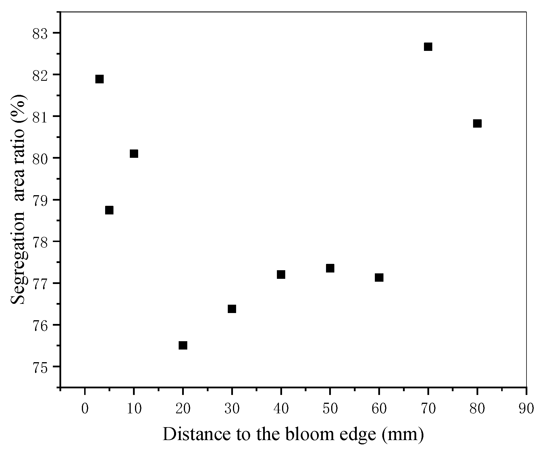
• Calculated results show that the velocity magnitude decreases from continuous casting bloom margin toward the center as a whole, and it decreases in the central zone first, then shows an increasing trend, and decreases again finally, which is in correspondence with segregation morphology. Besides the chilled zone, the velocity magnitude of the interdendritic fluid flow in the inner curve side is higher than that in the outer curve side. The velocity magnitude and related fluctuation is higher under 20 °C. Moreover, it is indicated that the fluctuation extent of SDAS is more relevant with interdendritic fluid flow, although the SDAS magnitude is mainly determined by the cooling rate.
• Meanwhile, on the basis of the magnitude and direction of velocity, there is a positive correlation between segregation area ratio and the effective ratio between interdendritic flow velocity and growth velocity, especially in equiaxed grain zones.
• On the whole, the model is demonstrated as a useful approach for determining the velocity of interdendritic fluid flow. The velocity distribution and associated defects formation in two or three-dimensional multiscale space can be better understand based on this model.

References

1. Kerr, R.; Woods, A.W.; Worster, M.; Huppert, H.E. Disequilibrium and macrosegregation during solidification of a binary melt. Nature 1989, 340, 357–362. [Google Scholar] [CrossRef]
2. Pickering, E.J. Macrosegregation in Steel Ingots: The Applicability of Modelling and Characterisation Techniques. ISIJ Int. 2013, 53, 935–949. [Google Scholar] [CrossRef] [Green Version]
3. Combeau, H.; Založnik, M.; Hans, S.; Richy, P.E. Prediction of Macrosegregation in Steel Ingots: Influence of the Motion and the Morphology of Equiaxed Grains. Met. Mater. Trans. A 2009, 40, 289–304. [Google Scholar] [CrossRef]
4. Li, D.; Chen, X.; Fu, P.; Ma, X.; Liu, H.; Chen, Y.; Cao, Y.; Luan, Y.; Li, Y. Inclusion flotation-driven channel segregation in solidifying steels. Nat. Commun. 2014, 5, 5572. [Google Scholar] [CrossRef] [Green Version]
5. Flemings, M.C.; Nero, G.E. Macrosegregation: Part 1. Trans. Metall. Soc. AIME 1967, 239, 1449–1461. [Google Scholar]
6. Flemings, M.C. Our Understanding of Macrosegregation. Past and Present. ISIJ Int. 2000, 40, 833–841. [Google Scholar] [CrossRef]
7. Beckermann, C. Modelling of macrosegregation: Applications and future needs. Int. Mater. Rev. 2002, 47, 243–261. [Google Scholar] [CrossRef]
8. Poirier, D.; Ocansey, P. Permeability for flow of liquid through equiaxial mushy zones. Mater. Sci. Eng. A 1993, 171, 231–240. [Google Scholar] [CrossRef]
9. Brown, S.; Spittle, J.; Jarvis, D.; Walden-Bevan, R. Numerical determination of liquid flow permeabilities for equiaxed dendritic structures. Acta Mater. 2002, 50, 1559–1569. [Google Scholar] [CrossRef]
10. Bernard, D.; Nielsen, Ø.; Salvo, P.L. Cloetens, Permeability assessment by 3D interdendritic flow simulations on microto-mography mappings of Al–Cu alloys. Mater. Sci. Eng. A 2005, 392, 112–120. [Google Scholar] [CrossRef]
11. Santos, R.; Melo, M. Permeability of interdendritic channels. Mater. Sci. Eng. A 2005, 391, 151–158. [Google Scholar] [CrossRef]
12. Khajeh, E.; Maijer, D.M. Physical and numerical characterization of the near-eutectic permeability of aluminum–copper alloys. Acta Mater. 2010, 58, 6334–6344. [Google Scholar] [CrossRef]
13. Mitraa, S.; Mansori, M.; Castro, A.; Costin, M. Study of the evolution of transport properties induced by additive processing sand mold using X-ray computed tomography. J. Mater. Process. Technol. 2020, 277, 116495. [Google Scholar] [CrossRef] [Green Version]
14. Takaki, T.; Sakane, S.; Ohno, M.; Shibuta, Y.; Aoki, T. Permeability prediction for flow normal to columnar solidification struc-tures by large scale simulations of phase field and lattice Boltzmann methods. Acta Mater. 2019, 164, 237–249. [Google Scholar] [CrossRef]
15. Koshikawa, T.; Bellet, M.; Gandin, C.-A.; Yamamura, H.; Bobadilla, M. Experimental study and two-phase numerical modeling of macrosegregation induced by solid deformation during punch pressing of solidifying steel ingots. Acta Mater. 2017, 124, 513–527. [Google Scholar] [CrossRef]
16. Pakanati, A.; Tveito, K.O.; M’Hamdi, M.; Combeau, H.; Založnik, M. Application of an Equiaxed Grain Growth and Transport Model to Study Macrosegregation in a DC Casting Experiment. Met. Mater. Trans. A 2019, 50, 1773–1786. [Google Scholar] [CrossRef]
17. Sengupta, J.; Leung, J.; Leung, J. Bridging the gap: MXRF technique rapidly maps centerline segregation. Iron Steel Technol. 2017, 7, 66–74. [Google Scholar]
18. Tsuchinaga, M.; Abe, S. The Pickling Process of Hot Rolled Ferritic Stainless Steel in Sulfuric Acid and Nitric Acid Solution. Tetsu-to-Hagane 2006, 92, 10–15. [Google Scholar] [CrossRef] [Green Version]
19. Preßlinger, H.; Ilie, S.; Reisinger, P.; Schiefermüller, A.; Pissenberger, A.; Parteder, E.; Bernhard, C. Methods for Assessment of Slab Centre Segregation as a Tool to Control Slab Continuous Casting with Soft Reduction. ISIJ Int. 2006, 46, 1845–1851. [Google Scholar] [CrossRef] [Green Version]
20. Hou, Z.; Guo, D.; Cao, J.; Chang, Y. A method based on the centroid of segregation points: A Voronoi polygon application to solidification of alloys. J. Alloys Compd. 2018, 762, 508–519. [Google Scholar] [CrossRef]
21. Abraham, S.; Cottrel, J.; Raines, J.; Wang, Y.; Bodnar, R.; Wilder, S.; Thomas, J.; Peters, J. Development of an Image Analysis Technique for Quantitative Evaluation of Centerline Segregation in As-Cast Products. Iron Steel Technol. 2017, 8, 148–157. [Google Scholar]
22. Kazakov, A.; Kiselev, D.; Pakhomova, O. Microstructural Quantification for Pipeline Steel Structure-Property Relationships. CIS Iron Steel Rev. 2012, 1, 4–12. [Google Scholar]
23. Hou, Z.; Guo, Z.; Guo, D.; Cao, J. A new method for carbon content distribution based on grayscale image of casting blank macrostructure in carbon steel. J. Iron Steel Res. 2019, 31, 620–627. [Google Scholar]
24. Thomas, T.R. Rough Surfaces, 2nd ed.; Imperial College Press: London, UK, 1999. [Google Scholar]
25. Howell, D.; Behrends, B. A review of surface roughness in antifouling coatings illustrating the importance of cutoff length. Biofouling 2006, 22, 401–410. [Google Scholar] [CrossRef]
26. Bowe, T.F.; Brody, H.D.; Flemings, M.C. Measurement of solute redistribution in dendritic solidification. Trans. Metall. Soc. AIME 1966, 236, 624–634. [Google Scholar]
27. Burton, J.A.; Prim, R.C.; Slichter, W.P. The Distribution of Solute in Crystals Grown from the Melt. Part I. Theoretical. J. Chem. Phys. 1953, 21, 1987–1991. [Google Scholar] [CrossRef]
28. Schaffnit, P.; Stallybrass, C.; Konrad, J.; Stein, F.; Weinberg, M. A Scheil–Gulliver model dedicated to the solidification of steel. Calphad 2015, 48, 184–188. [Google Scholar] [CrossRef]
29. Dong, H.; Lee, P. Simulation of the columnar-to-equiaxed transition in directionally solidified Al–Cu alloys. Acta Mater. 2005, 53, 659–668. [Google Scholar] [CrossRef]
30. Ryan, T.P. Modern Regression Theory, 2nd ed.; John Wiley & Sons: Hoboken, NJ, USA, 2009. [Google Scholar]
31. Trivedi, R.; Kurz, W. Dendritic Growth. Int. Mater. Rev. 1994, 39, 49–74. [Google Scholar] [CrossRef]
32. Byron, R.; Bird, W.E.; Stewart, E.N. Lightfoot, Transport Phenomena, 2nd ed.; John Wiley & Sons: New York, NY, USA, 2002. [Google Scholar]
33. Choudhary, S.K.; Ganguly, S. Morphology and Segregation in Continuously Cast High Carbon Steel Billets. ISIJ Int. 2007, 47, 1759–1766. [Google Scholar] [CrossRef] [Green Version]
34. Hou, Z.; Jiang, F.; Cheng, G. Solidification Structure and Compactness Degree of Central Equiaxed Grain Zone in Continuous Casting Billet Using Cellular Automaton-Finite Element Method. ISIJ Int. 2012, 52, 1301–1309. [Google Scholar] [CrossRef] [Green Version]
35. Schlichting, H.; Gersten, K. Boundary Layer Theory, 9th ed.; Springer: Berlin/Heidelberg, Germany, 2017. [Google Scholar]
36. Kurz, W.; Fisher, D.J. Fundamentals of Solidification, 4th ed.; Trans Tech Publications Ltd.: Zurich, Switzerland, 1998. [Google Scholar]
37. Isobe, K. Formation Mechanisms of Several Kinds of Segregation on Continuous Casting of Bloom. Tetsu-to-Hagane 2012, 98, 405–414. [Google Scholar] [CrossRef] [Green Version]
38. Natsume, Y.; Takahashi, D.; Kawashima, K.; Tanigawa, E.; Ohsasa, K. Evaluation of Permeability for Columnar Dendritic Structures by Three-dimensional Numerical Flow Analysis. ISIJ Int. 2014, 54, 366–373. [Google Scholar] [CrossRef] [Green Version]
39. Hou, Z.; Cao, J.; Chang, Y.; Wang, W.; Chen, H. Morphology Characteristics of Carbon Segregation in Die Steel Billet by ESR Based on Fractal Dimension. Acta Metall. Sin. 2017, 53, 769–777. [Google Scholar]
40. Takahashi, T.; Ichikawa, K.; Kudou, M.; Shimahara, K. The Effect of Fluid Flow on the Macrosegregation in Steel Ingot. Tetsu-to-Hagane 1975, 61, 2198–2213. [Google Scholar] [CrossRef] [Green Version]
41. Miyazawa, K.; Schwerdtfeger, K. Macrosegregation in continuously cast steel slabs: Preliminary theoretical investigation on the effect of steady state bulging. Archiv für das Eisenhüttenwesen 1981, 52, 415–422. [Google Scholar] [CrossRef]
42. Huang, J.T.; He, J.C. Numerical simulation of steel solidification and electromagnetic brake in the billet mold. Acta Metall. Sin. 2001, 37, 281–286. [Google Scholar]
43. Kajatani, T.; Drezet, J.-M.; Rappaz, M. Numerical simulation of deformation-induced segregation in continuous casting of steel. Met. Mater. Trans. A 2001, 32, 1479–1491. [Google Scholar] [CrossRef] [Green Version]
Figure 1. Schematic of curved continuous casting machine: GCr15 molten steel is poured into the mold through the top tundish, then solidifying along the casting direction. The bloom size is 220 mm × 220 mm. MEMS and FEMS are mold and final electromagnetic stirrings, and the conditions of the electromagnetic stirring are the same under different superheats. The sample is obtained by cutting along the transverse section of the bloom after finishing solidification.
Metals 11 00927 g001
Figure 2. Macrostructure of GCr15 steel bloom sample: (a) whole etched surface at 20 °C (220 mm × 220 mm); (b) measured etched surface at 20 °C (12.5 mm × 220 mm); (c) whole etched surface at 35 °C (220 mm × 220 mm); (d) measured etched surface at 35 °C (12.5 mm × 220 mm).
Metals 11 00927 g002
Figure 3. Schematic of measurement location of etched surface height at each position in inner or outer curve side for velocity magnitude calculation. (The bloom edge is corresponding to that in Figure 2. The distance to the bloom edge at A–M positions are 1, 3, 5, 10, 20, 30, 40, 50, 60, 70, 80, 90 and 100 mm, respectively. From down to up, the measuring length is 12.5 mm at each position where 50,001 measurement points are contained).
Metals 11 00927 g003
Figure 4. Schematic of measurement location of etched surface height at left side and right side of each position for velocity direction calculation. (α and β are the horizontal measuring line of the left side and the right side at each position. From left to right, the measuring length is 1.0 mm at each side where 1001 measurement points are contained. The vertical dashed arrow corresponds to same arrow in Figure 3).
Metals 11 00927 g004
Figure 5. The original heights and the filtered heights ( h e s ) at A position (1 mm to bloom edge) in the outer curve side (O) under 35 °C superheat: (a) original height, (b) filtered height. (The measuring length is 12.5 mm, and there are 50,001 points with 0.25 μm intervals along the distance. The arrow line represents the whole changing trend with the distance).
Metals 11 00927 g005
Figure 6. The etched surface heights ( h e s ) at A to M positions in the inner curve side (I) under 20 °C superheat. (am) are A–M positions. (The measuring length is 12.5 mm, and there are 50,001 points with 0.25 μm intervals along the distance).
Metals 11 00927 g006aMetals 11 00927 g006bMetals 11 00927 g006c
Figure 7. The etched surface heights ( h e s ) of left side (α) and right side (β) at B position (3 mm to bloom edge) in the inner curve side under 20 °C superheat: (a) left side, (b) right side. (The measuring length of each side is 1.0 mm, and there are 1001 points with 0.25 μm intervals along the distance).
Metals 11 00927 g007
Figure 8. The etched surface heights ( h e s ) of the left side (α) and right side (β) at C position (5 mm to bloom edge) in the inner curve side under 20 °C superheat: (a) left side, (b) right side. (The measuring length of each side is 1.0 mm, and there are 1001 points with 0.25 μm intervals along the distance).
Metals 11 00927 g008
Figure 9. Correlation between the segregating element contents and the etched surface heights at F position in the inner curve of Scheme 20 °C along horizontal dashed arrow corresponds to the same arrow in Figure 3: (a) macrostructure marked in the red rectangular area in Figure 4 photographed by a SELP1650 digital camera; (b) etched surface height ( h e s ) along horizontal dashed arrow in Figure 9a. (1), (2) and (5) points have a relative maximum value of height. (3), (4) and (6) points have a relative minimum value of height.
Metals 11 00927 g009
Figure 10. Variation of the dimensionless quantity of carbon content C d as a function of liquid fraction during solidification. (The results at A position in the outer curve side under 35 °C are displayed as an example).
Metals 11 00927 g010
Figure 11. Example of the distribution of dimensional quantity of carbon content C d with 0 to 0.7 liquid fraction and its fitted equation. (The equation determination coefficient is 0.9681, which indicates that the fitted power-law equation can express the distribution very well).
Metals 11 00927 g011
Figure 12. Calculation flowchart for magnitude of interdendritic fluid flow velocity V i f f using the etched surface height of the actual metal ingot.
Metals 11 00927 g012
Figure 13. Schematic of degree θ of V i f f direction on xz plane (marked by blue ellipse line) in three-dimensional space. (Considering surface from inner curve side to outer curve side as x-positive axis, the grain growth direction from bloom left edge to center as y-positive axis, and casting direction as z-positive axis).
Metals 11 00927 g013
Figure 14. Calculation flowchart for direction degree θ of interdendritic fluid flow velocity V i f f using the etched surface height of the actual metal ingot.
Metals 11 00927 g014
Figure 15. The magnitude of interdendritic fluid flow velocity V i f f at different positions in the inner curve side (I) and outer curve side (O) of whole zone under 20 and 35 °C.
Metals 11 00927 g015
Figure 16. The magnitude of interdendritic fluid flow velocity V i f f at different positions in different zones: (a) chill zone, (b) middle zone, (c) central zone (The velocity magnitude in the central zone decreases firstly, then shows an increasing trend and decreases again finally as shown by arrow line in Figure 15c).
Metals 11 00927 g016
Figure 17. Average value and standard deviation of interdendritic fluid flow velocity V i f f magnitude of middle and central zones in the inner curve side and the outer curve side under 20 °C and 35 °C: (a) average value, (b) standard deviation.
Metals 11 00927 g017
Figure 18. Increasing proportion of average magnitude of interdendritic fluid flow velocity V i f f of the inner curve side compared to that of outer curve side at different zones.
Metals 11 00927 g018
Figure 19. The average magnitude of interdendritic fluid flow velocity V i f f of inner and outer curve sides at chill, middle, and central zones and average standard deviation of velocity magnitude of all sides under 20 °C and 35 °C: (a) average velocity magnitude, (b) average standard deviation.
Metals 11 00927 g019
Figure 20. Secondary arm spacings (SDASs) at different locations and corresponding average values under 20 and 35 °C.
Metals 11 00927 g020
Figure 21. Differences of standard deviation between (left) side height and (right) side height ( E V D ) at different positions. (The standard deviation at G position has the largest negative value).
Metals 11 00927 g021
Figure 22. The magnitude and direction degree θ of interdendritic fluid flow velocity V i f f at different positions. (The direction degree θ at G position is zero).
Metals 11 00927 g022
Figure 23. Macrostructures at 10 positions (BK) in the inner curve side under 20 °C whose distances to the bloom edges are 3, 5, 10, 20, 30, 40, 50, 60, 70, and 80 mm, respectively. (The location relative to the measuring line is marked by a red rectangle in Figure 4).
Metals 11 00927 g023
Figure 24. Segregation area ratios of 10 macrostructure positions in Figure 23.
Metals 11 00927 g024
Figure 25. Relationship between segregation area ratio and the effective ratio between interdendritic flow velocity and growth velocity ( V i f f / M x ) e . The equiaxed grain positions are marked by the dashed line and they show a linear increasing trend along the arrow. The columnar grain positions are marked by the dot-dash line; they also show a minor increasing trend if excluding E position marked by the full line.
Metals 11 00927 g025
Figure 26. The measured k E by the new approach (the discrete dots of different shapes) and the corresponding empirical k E by Equation (23) (the continuous full line) under different magnitudes of interdendritic fluid flow velocity V i f f . (a) A, B, C positions, (b) D, E, F positions, (c) G, H, I positions, (d) J, K, L, M positions. (The distance to the bloom edges at A, B, C, D, E, F, G, H, I, J, K, L and M positions are 1, 3, 5, 10, 20, 30, 40, 50, 60, 70, 80, 90, and 100 mm, respectively).
Metals 11 00927 g026