Article

Prediction on Mechanical Properties of Non-Equiatomic High-Entropy Alloy by Atomistic Simulation and Machine Learning

1
International Joint Laboratory for Light Alloys (MOE), College of Materials Science and Engineering, Chongqing University, Chongqing 400044, China
2
Shenyang National Laboratory for Materials Science, Chongqing University, Chongqing 400044, China
3
Educational Physiology Laboratory, The University of Tokyo, Tokyo 113-0033, Japan
4
Department of Computing, Imperial College London, London SW72AZ, UK
5
Department of Materials Engineering, The University of Tokyo, Tokyo 113-8656, Japan
*
Author to whom correspondence should be addressed.
These authors contributed equally.
Metals 2021, 11(6), 922; https://doi.org/10.3390/met11060922
Submission received: 13 May 2021 / Revised: 1 June 2021 / Accepted: 3 June 2021 / Published: 6 June 2021

Abstract

:
High-entropy alloys (HEAs) with multiple constituent elements have been extensively studied in the past 20 years, due to their promising engineering application. Previous experimental and computational studies of HEAs focused mainly on equiatomic or near equiatomic HEAs. However, there is probably far more treasure in those non-equiatomic HEAs with carefully designed composition. In this study, the molecular dynamics (MD) simulation combined with machine learning (ML) methods was used to predict the mechanical properties of non-equiatomic CuFeNiCrCo HEAs. A database was established based on a tensile test of 900 HEA single-crystal samples by MD simulation. Eight ML models were investigated and compared for the binary classification learning tasks, ranging from shallow models to deep models. It was found that the kernel-based extreme learning machine (KELM) model outperformed others for the prediction of yield stress and Young’s modulus. The accuracy of the KELM model was further verified by the large-sized polycrystal HEA samples. The results show that computational simulation combined with ML methods is an efficient way to predict the mechanical performance of HEAs, which provides new ideas for accelerating the development of novel alloy materials for engineering applications.

Graphical Abstract

1. Introduction

The concept of “high-entropy alloys” (HEAs), in which metals are mixed by five or more elements in equiatomic or near-equiatomic proportions, was proposed by Yeh and co-workers [1], and independently by Cantor and co-workers [2] in 2004. After this, HEAs have been extensively studied by researchers due to their advanced properties in many aspects [3,4]. Compared to conventional alloys, which contain one and rarely two base elements, HEAs have proven to show many superior mechanical properties, including excellent strength, exceptional ductility and fracture toughness at cryogenic temperatures, superior mechanical performance at high temperatures, super-paramagnetism and superconductivity [5]. Some recent high-profile studies have shown that well-designed HEAs exhibit superior mechanical properties that can overcome the longstanding conundrum of the strength–ductility trade-off in materials [6,7,8]. The excellent mechanical properties of HEA make it an advanced structural material, with promising engineering applications.
HEA is a large field with a countless number of new alloy systems. If five elements were randomly selected from a pool of 118 elements to form an alloy, the number of combinations could reach about 200 million using the combination theory. If only 38 transition metals were considered, the number of new alloys would still be as high as about 500,000 [5]. Due to their considerable structural and functional potential, as well as the richness of design, different combinations of the elements and their compositions need to be explored to understand the potentials of HEAs further. Our understanding of these new alloys is still very limited. The equiatomic composition is usually the easiest access to a new alloy system, and the HEAs with equiatomic compositions were intensively investigated by many of the previous research works [5]. However, the equiatomic HEAs probably do not possess the best combination of properties. For example, a novel, single-phase, non-equiatomic Fe40Mn27Ni26Co5Cr2 (at.%) HEA was reported with exceptional phase stability and excellent tensile ductility [9]. The bulk nanocrystalline Co25Ni25Fe25Al7.5Cu17.5 (at.%) HEA can exhibit a compressive yield strength of about 1.8 GPa, which is higher than the yield strength of most previously reported face-centered cubic (fcc) structured HEAs [10]. As suggested by Yeh, the pioneer of HEAs, ‘there is probably far more treasure in those non-equimolar alloys with carefully designed composition and tailored microstructures’ [11].
A good method is to start with equiatomic HEA and then change the composition of the consisted elements, according to the target properties for the design of a new non-equiatomic HEA system. An empirical trial-and-error approach requires a large amount of time and cost of designing, it is impossible to evaluate such huge numbers of the HEA system in the available time by traditional methods, especially for experimental methods. High-throughput computational material design integrated with advanced machine learning (ML) methods provides new tools for exploring the vast space of possible materials and finding the required properties. This field represents an emerging and dynamic scientific activity that has contributed significantly to the discovery of new materials [12,13,14,15,16]. The basic strategy is to combine the high-throughput computation results or materials databases with intelligent data analysis techniques, giving full play to its advantages to seeking target performance. The composition design of HEA provides an ideal platform for developing, validating and applying these new techniques.
In this work, molecular dynamics (MD) simulation was combined with different ML methods to predict the mechanical properties of HEAs with changes in the elemental compositions. The schematic diagram is shown in Figure 1. Firstly, the mechanical responses of 900 single-crystal CuFeNiCrCo samples with different compositions (at.%) were obtained by MD simulations. Based on the MD results, a database was established to describe the relationship between element composition and mechanical properties of the tested HEA samples. Secondly, the overall dataset was divided into train, development (dev) and test sets. Eight ML models were investigated and compared for a binary classification task. The composition of the five elements was used to give a prediction on yield stress and elastic modulus of HEA. Finally, the large polycrystal CuFeNiCrCo samples with different compositions were constructed. The well-trained ML model, based on single-crystal samples, was used to predict the mechanical responses of the polycrystal samples. The prediction from the kernel-based extreme learning machine (KELM) model was in good agreement with the calculated results from the MD simulation. This contribution shows that computational study combined with ML methods is an efficient way to predict the mechanical properties of HEAs.

2. Methods

2.1. Simulation Sample

For the HEA single-crystal, the 900 small-size samples were generated without initial structural defects. The length of each side of the cube sample is approximately 10 nm, and the number of atoms is about 100,000. The current sample size was controlled for a consideration of the computational efficiency for high throughput MD simulation, and ensures the observation of primary nucleation of dislocations in the grain [17]. The large-size HEA polycrystal samples were constructed using the Voronoi construction method containing 16 grains with random crystallographic orientations. The mean grain size is 27.4 nm, and the total number of atoms is over 10 million. Atoms of the five elements are uniformly distributed in the single-crystal and polycrystal HEA samples [18]. Both single-crystal and polycrystal samples were constructed with a fcc phase. HEAs with the fcc phase have been widely researched in previous experimental studies, and this has been found to be a stable phase of the similar alloy system as CuFeNiCrCo [5].
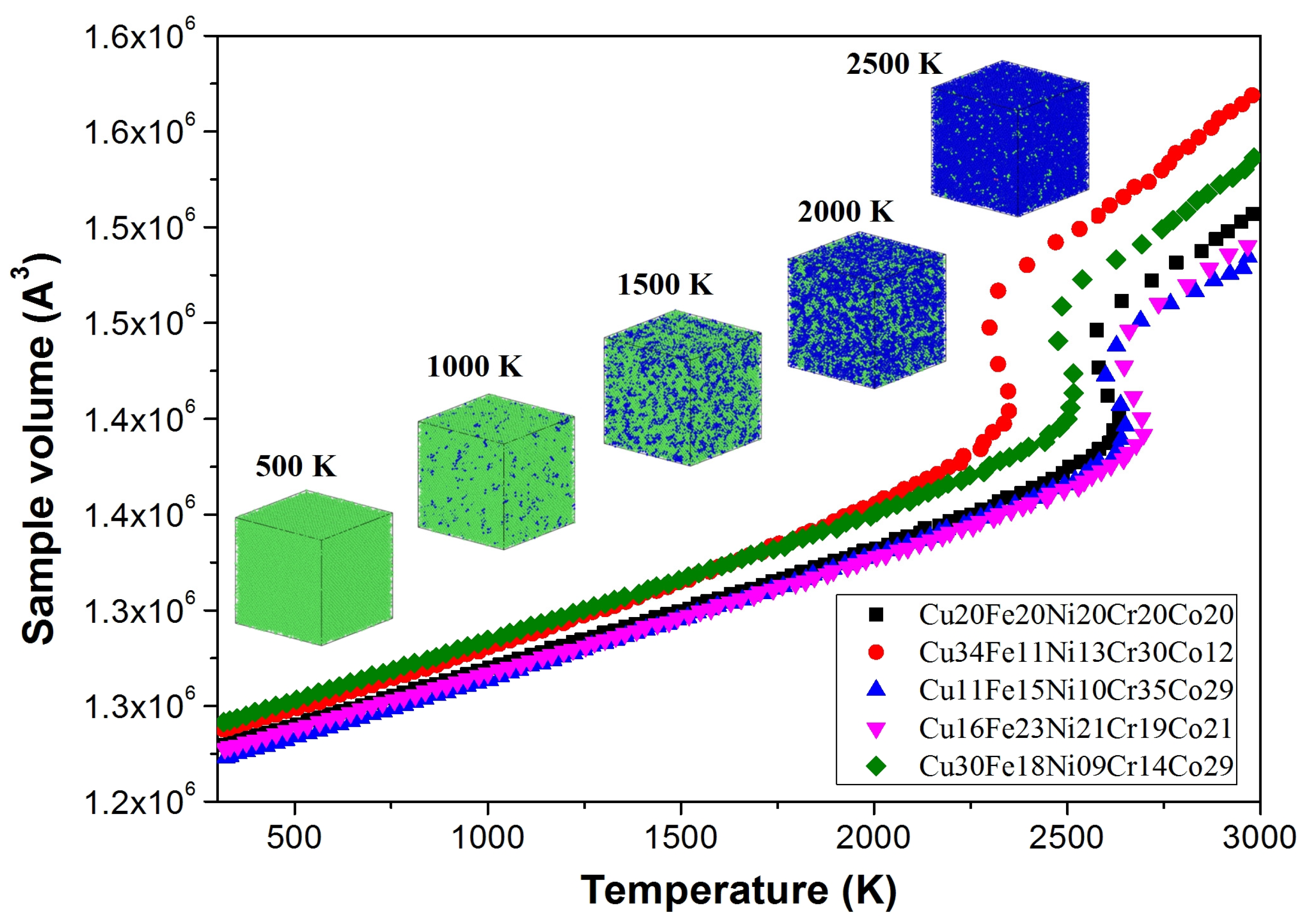
The phase stability of the simulation sample was further examined by gradually raising the system temperature. Before the heating process, the HEA sample was firstly relaxed to an equilibrium configuration at 300 K in the canonical ensemble NVT (constant atom number, constant box volume and constant temperature). Then, the temperature gradually increases from ambient temperature (300 K) to high temperature (3000 K) in the isothermal-isobaric ensemble (NPT). As shown in Figure 2, the HEA samples with different element compositions were tested, including an equiatomic sample and four non-equiatomic samples. The total volume of the system was monitored during the heating process. The inserted snapshots show the atomic configurations of the Cu30Fe18Ni9Cr14Co29 sample at different temperature levels. Atoms are coloured by common neighbour analysis (CNA) method, where the green atoms are in fcc structure, and the blue atoms represent a disordered structure. It was found that the fcc phase of the HEA sample has not changed below 1000 K. From 1500 to 2000 K, the disordered atoms (blue atoms) increased considerably. The first-order phase transition (solid to liquid) was observed at about 2500 K, where the sample volume shows a sudden jump. The other four simulated samples in Figure 2 show a similar process, although the melting temperature varies depending on the composition of the elements.

2.2. MD Simulation

MD simulations were performed using the parallel molecular dynamics package LAMMPS [19], with the embedded atom method (EAM) interatomic potentials developed for the CuFeNiCrCo HEA system [20]. The interatomic potential can accurately reflect the basic structural and physical characteristics of the five components, including the lattice constant, cohesive energy and elastic modulus [20]. In particular, the interatomic potential can present a large variation in stacking fault energies of the constituent elements, both stable and unstable, which is significant for the study of dislocation behaviour, and therefore the mechanical properties of the alloy system.
The equilibrium structure of the HEA sample was obtained after an initial energy minimisation with a standard conjugate gradient algorithm, and then followed a system annealing at the temperature of 300 K for 100 ps [21,22]. Periodic boundary conditions were applied to all directions, and atomic vibration and change in sample dimensions were allowed during the simulation. The fcc lattice structure of the samples was maintained after system annealing in an isobaric-isothermal (NPT) environment. In order to test the mechanical properties of HEA samples with different compositions, the uniaxial tension was applied in one direction, while the pressure along the other two directions was kept at zero in the NPT ensemble (T = 300 K). In particular, when conducting the dynamic tension simulation, we not only randomly changed the composition of the elements in the alloy system, but also considered an important physical index of materials, namely the anisotropy of the mechanical properties. Here, nine crystallographic orientations were deliberately selected to test the mechanical properties of HEA samples. These orientations are the representative orientations in the texture of materials, including the vertex position ([100], [110], [111]), edge position ([210], [211], [221]) and internal position ([321], [821], [876]) of the inverse pole figure for material textures. The deformation strain was set at a constant rate of 5 × 10⁸ s−1, and the timestep was set as 1 fs throughout the work. The short time duration to which MD simulations are inherently limited is particularly relevant to the simulation of plastic deformation. As a consequence of this, MD simulations always involve extremely high strain rates of typically 107 to 109 s−1. The strain rate and timestep set in this study are frequently used parameter in MD simulations. System strain was derived from the positions of the periodic boundaries along the loading direction, and the system stress was attained by calculating the pressure of the entire system of atoms. All the atomic figures in this study are illustrated by the visualisation tool OVITO [23].

2.3. ML Method

For metallic materials, the nucleation of the first set of dislocations corresponds to the theoretical yield strength, and represents the beginning of the plastic deformation [24]. It also plays a significant role in the contribution of material-hardening mechanisms, and hence can be used to guide the design and optimisation of alloy composition. Therefore, yield stress (YS) was chosen as the first learning target for ML. On the other hand, Young’s modulus is an intrinsic mechanical property, mainly determined by the elements of their constitutions and crystal structures. For the conventional one-element principal alloys, Young’s modulus is mainly controlled by the dominant element. In contrast, for HEAs, Young’s modulus can be very different from any of the constituent elements in the alloys [25]. Here, Young’s modulus (E) was chosen as the second learning target for ML.
In the ML task, the composition of the five elements CuFeNiCrCo was used as input feature to predict the mechanical properties. The principal concept of HEAs is based on designing the alloys with multiple principal elements, ranging from 5 to 35 atomic percent with a target to form single-phase solid solutions arising from the high entropy of the system [1]. Therefore, when randomly assigning the proportion of the five elements, the upper limit of each element was controlled to be 35%, and the lower limit to be 5%. The mechanical properties (YS and E) were set as output features, and the binary classification of the output values is the learning target.
In particular, the traditional material design by ML is only based on the design of a pure mathematical algorithm, while the intrinsic structural and physical properties of the material are not considered. In this way, ML usually requires large data information, and may result in uneven learning samples in terms of the special properties of materials. In this study, when establishing the database, the anisotropy of the mechanical properties of materials was considered and nine representative crystallographic orientations were selected to test the mechanical properties of HEA samples. MD simulations on each orientation contains a result of the equiatomic HEA sample and 100 results of the non-equiatomic HEA samples based on different element compositions.
There are three main paradigms in ML: supervised learning, unsupervised learning and reinforcement learning. Our task is to predict the mechanical properties (output features) of the HEA samples through element composition as the input features; hence, the supervised learning paradigm is selected. Eight ML models were investigated and compared, ranging from classic (shallow) models to deep models, including Naïve Bayes (NB) [26], linear discriminant analysis (LDA) [27], k-Nearest Neighbour (k-NN) [28], support vector machine (SVM) [29], extreme learning machine (ELM) [30], kernel-based extreme learning machine KELM [31], deep neural network (DNN) [32] and stacked auto-encoders (SAEs) [33].

3. Results and Discussion

3.1. Mechanical Response of HEA Single-Crystal

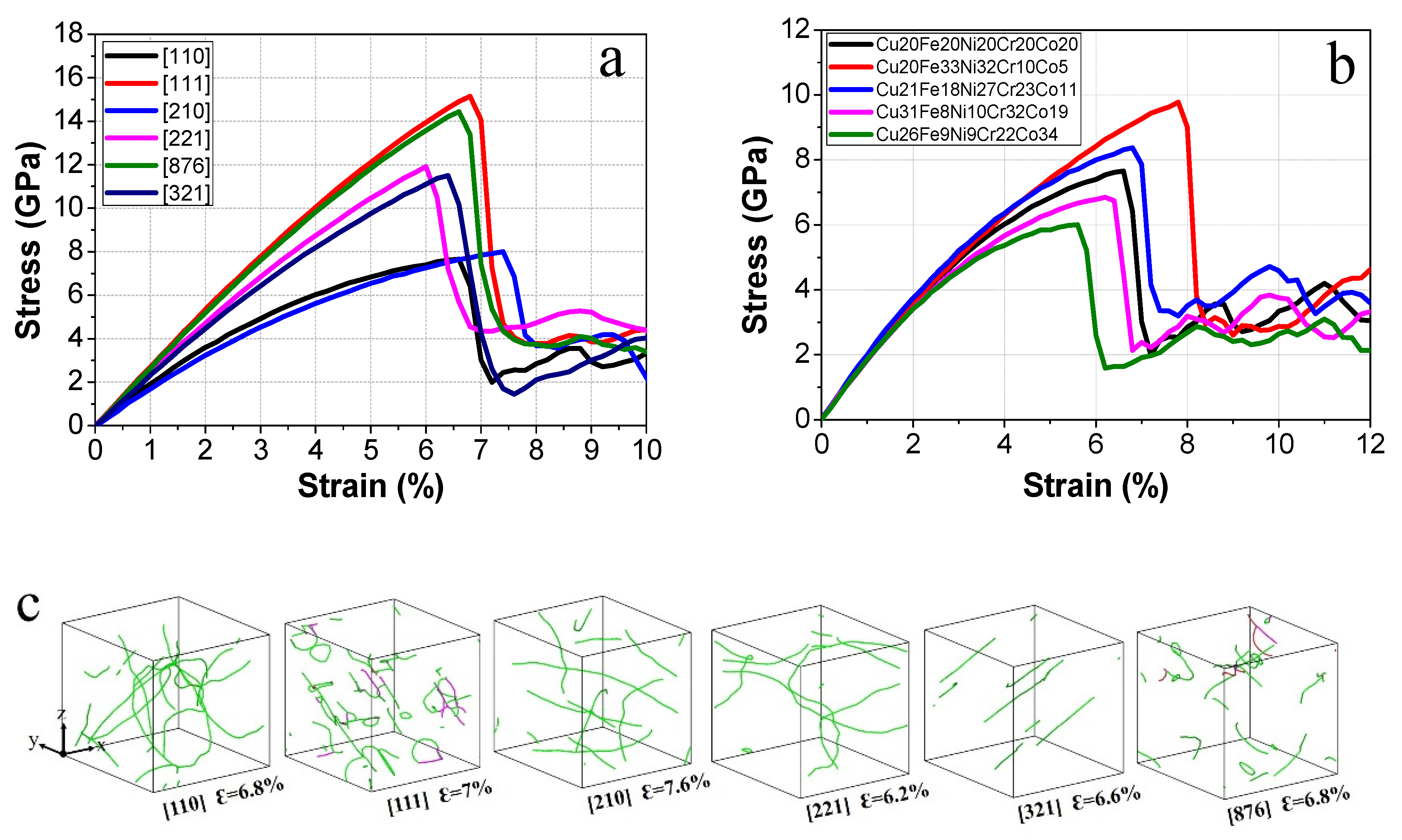
The mechanical responses of the equiatomic CuFeNiCrCo samples with different crystallographic orientations under uniaxial tension at 300 K are shown in Figure 3a. Young’s modulus for each orientation is obtained from the linear portion of its corresponding stress-strain between 0 and 0.5% strain. Theoretically, the nucleation of the first set of dislocations corresponds to the yield strength of materials [24]. Figure 3c shows the snapshots of the nucleation of the first set of dislocations in the single-crystal samples with different orientations. The dislocations are extracted by the dislocation extraction algorithm (DXA) algorithm [34], wherein the different colours represent different types of dislocations. By comparing the tensile strain, it was found that the dislocation nucleation event occurs near the peak of the stress-strain curve. Therefore, according to previous MD studies, the peak stress on the stress-strain curve is defined as the yield stress [35,36,37]. The mechanical response shows an elastic anisotropy of the HEA samples with different crystal orientations. The tension along [111] orientation shows the maximum Young’s modulus of 268.96 GPa, while the [210] orientation has the minimum value of 169.07 GPa. Additionally, there are remarkable differences in yield stress for different orientations; the maximum yield stress is 15.14 GPa for [111] orientation, and the minimum value is 7.66 GPa for [110] orientation. Therefore, considering the anisotropy of the mechanical properties of materials can contain a wider range of information than simply considering the element composition when establishing a database, which is conducive to improving the reliability and applicability of an ML model in dealing with complex structural materials.
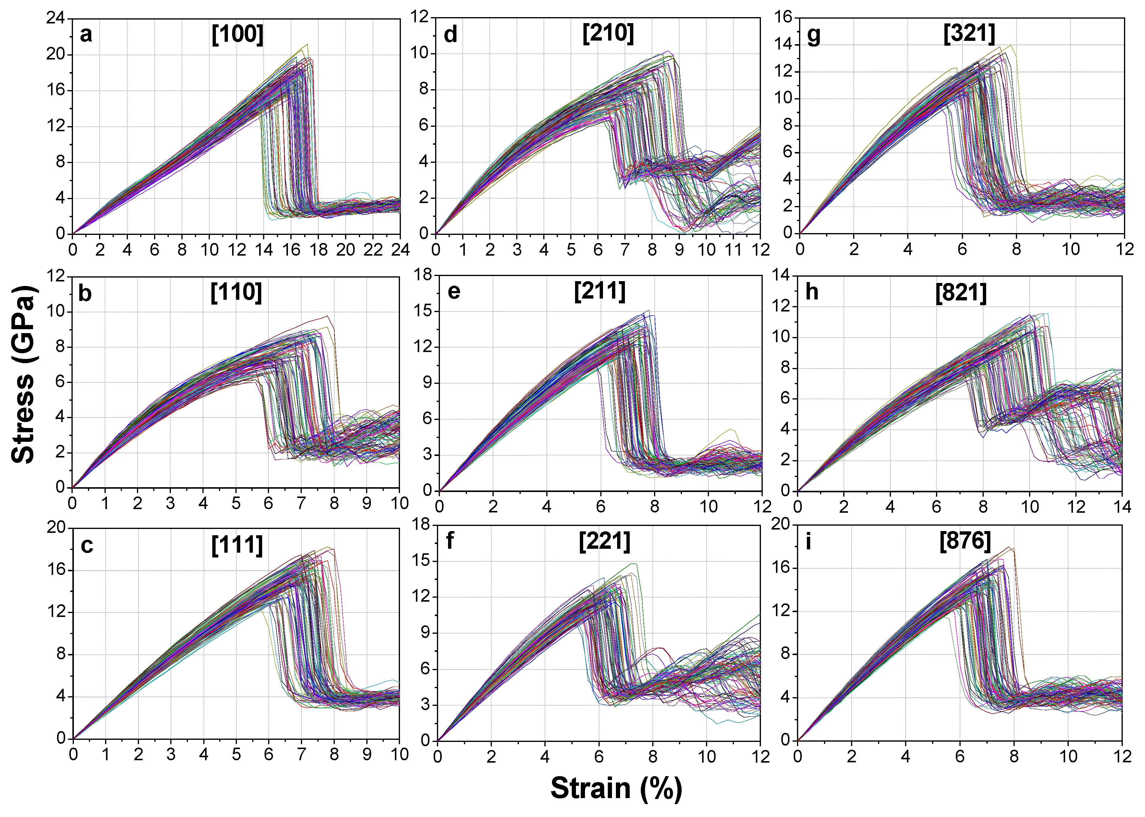
The stress-strain responses of the non-equiatomic HEA samples with different orientations are presented in Figure 4. For each orientation, the figure contains 100 results of the non-equiatomic HEA samples based on the random combination of the constituent elements. The results of the equiatomic HEA sample are also plotted for comparison. It is found that the yield stress and Young’s modulus of the equiatomic HEA sample are at a medium level for all tested orientations. For example, Figure 3b plots the stress-strain responses of five HEA samples with different element compositions along [110] orientation. The maximum Young’s modulus is 199.5 GPa for the Cu21Fe18Ni27Cr23Co11 sample, and the minimum value is 183.5 GPa for the Cu31Fe8Ni10Cr32Co19 sample. The maximum yield stress of 9.78 GPa is observed for the Cu20Fe33Ni32Cr10Co5 sample, and the Cu26Fe9Ni9Cr22Co34 sample has the minimum value of 6 GPa. For the equiatomic HEA sample, the yield stress (7.66 GPa) and Young’s modulus (192.3 GPa) are at a medium level among the five samples.
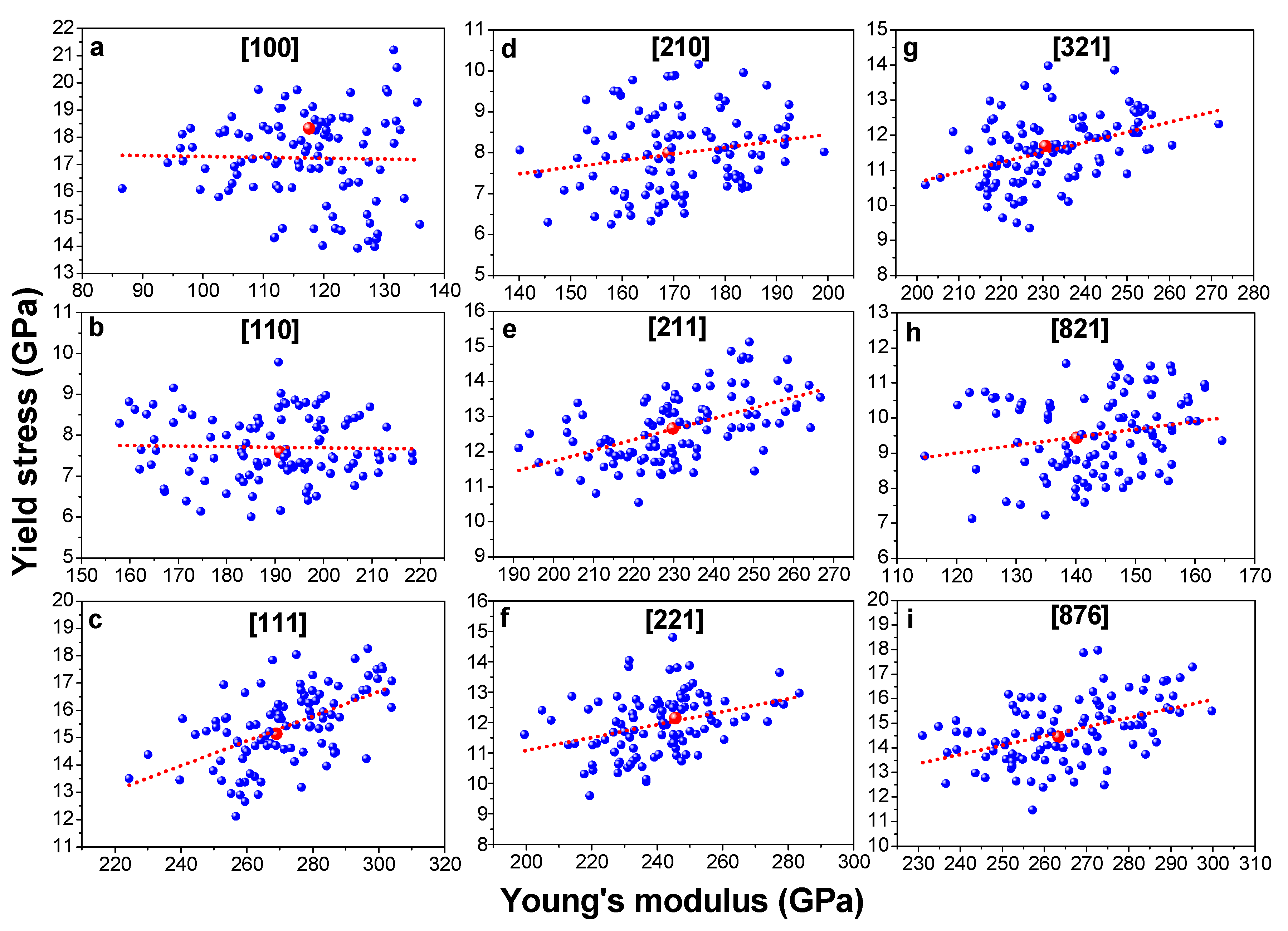
Two conclusions can be drawn from the above results. On the one hand, changing the proportions of elements can improve or decrease the mechanical properties of HEA samples, which provides an opportunity for achieving the required performance of HEA by optimising its element composition. On the other hand, the high Young’s modulus does not guarantee high yield stress. For the equiatomic HEA sample, the yield stress of [100] orientation is 18.26 GPa, which is more than twice than that of the [110] orientation (7.66 GPa). However, Young’s modulus of [100] orientation (118.7 GPa) is much lower than that of [110] orientation (192.27 GPa). For further illustration, Figure 5 plots the yield stress (Ys) as a function of Young’s modulus (E) of different CuFeNiCrCo samples under tension along different orientations. The fitting lines guide the general trend of the point sets. The scattered points indicate that there is no direct correlation between E and Ys of the HEA samples.
The lower correspondence between Young’s modulus and yield stress is mainly ascribed to the nonlinear elastic behaviour of materials under strain, either ‘elastic hardening’ or ‘elastic softening’ during dynamic tension in the elastic stage [38]. The yield stress is usually small accompanied by the elastic softening, while a high yield stress value can be achieved when the elastic hardening occurs. Although the yield stress generally increases with the increase of Young’s modulus for most orientations, the correspondence between the two values is not prominent. The independence of Young’s modulus and yield stress makes it necessary to predict the two mechanical properties by ML separately.

3.2. ML Models Training and Evaluation

Based on the MD simulations on the tensile responses of CuFeNiCrCo single-crystal samples, the quantitative relationship between element composition (input features) and the mechanical properties (Ys and E, output features) of HEA samples were obtained, and the database used for ML was constructed (see Supplementary Materials). In this section, eight ML models were investigated for the given tasks, ranging from shallow models to deep models. The overall dataset was split into train, development (dev) and test sets, which occupy 60, 20 and 20% of the whole instances, respectively. In order to eliminate the effects of outliers, all the input features (the element composition) were standardised using a z-score transformation before being fed into the ML models. The feature vectors were scaled to a distribution having an arithmetic mean of zero and a variance of one. Let x(n) be the composition vector of the n-th element in the high-entropy alloy data, and the values of x(n) were standardised as
x ˜ ( n ) = [ x ( n ) μ x ] / σ x
where μ x and σ x are the mean and the standard deviation of the vector x(n), respectively. The information was measured in the train set ( μ x and σ x ), and was applied to the dev and test sets.
Considering the imbalanced characteristic of our proposed database (i.e., the number of instances belonging to each class is unequal among the database), the unweighted average recall (UAR) was used as the main metric to evaluate model performance (Section S1). The UAR metric is regarded as more suitable and rigorous than the weighted average recall (WAR) for evaluating a model’s performance based on an imbalanced database [39]. On the other hand, the WAR, the sensitivity (Sens.), the specificity (Spec.), the precision (Prec.) and the F1-score are calculated as complementary evaluation metrics. The results of the complementary evaluation metrics are listed in Table 1. The hyper-parameters of all ML models are tuned and optimised on the dev set based on the performance (UAR). A grid-search strategy was used to decide the optimal hyper-parameter for a specific ML model. The detailed information of the grid-search strategy and the procedure of hyper-parameter optimisation are introduced in Section S2 [40,41,42,43]. When conducting the final evaluation, the data of the train and dev set are merged together to train the ML model within the optimised hyper-parameters, which are used to predict the output features (Ys and E) of the HEA samples in the test set.
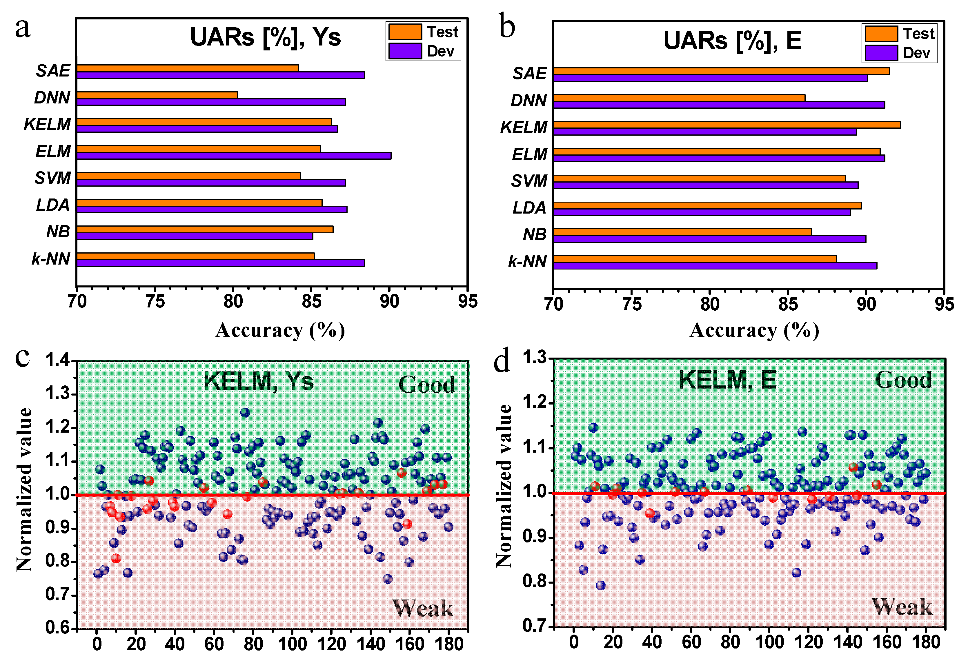
The achieved results (UARs in [%]) of the eight ML models for the learning task of yield stress (Ys) and Young’s modulus (E) are presented in Figure 6a,b. It is seen that most of the results are above 85.0% of UAR, indicating that the ML models perform efficiently for both of the two tasks. For the task of yield stress, the best UAR achieved on the test set is reached by the NB model (86.4%), while for the task of Young’s modulus, the KELM model takes the first place with a UAR of 92.2%. It is found that some simple ML models (e.g., NB, k-NN, LDA) can also show a good capacity in predicting the results; they perform well for both of the two tasks. It is reasonable to think that the relationship between the element composition (input features) and the mechanical properties (output features) of the HEA is sufficient to build ML models. Compared to the DNN model, a simple multi-layer perceptron structure without pre-training process in this study, the SAE model can learn more information inherited from the data itself in an unsupervised paradigm due to their pre-training process. Therefore, the SAE outperforms the general DNN for the two tasks on the test set. However, both of the two models have been constrained in this study, mainly due to the limited instance number of the small database for deep learning models. In contrast, ELM and its variant, KELM, are demonstrated to be more efficient in this study. Unlike the two deep models, the ELM and KELM models do not require to tune the parameters of the hidden nodes, which makes their training process much faster. Moreover, for a small size dataset in this study, ELM and KELM were able to execute efficiently while maintaining a fast training scheme. SVM is a popular and stable ML model that has been successfully applied to many tasks in the past decades. In this study, although SVM has shown some robustness and effectiveness, the results are not as good as ELM and KELM. It was indicated that, when using kernels, SVM is more likely to get sub-optimal solutions than KELM, which may lead to a negative result [44]. By comparing the UAR results, as well as other complementary evaluation metrics of the above models, it is believed that the KELM model has a better overall performance for the two learning tasks, and it is selected as the preferred ML model in the subsequent prediction studies.
To further demonstrate the effectiveness of the KELM model, Figure 6c,d plot the 180 predicted results on the test set by the KELM model. Firstly, the results of yield stress and Young’s modulus from MD simulations are divided into the two categories of ‘Good’ and ‘Weak’, respectively. The red line is the benchmark line defined by the values of the equiatomic sample, and the value is set as one. The 180 results of the non-equiatomic samples distributed along horizontal axis are normalised according to the benchmark value, and they are plotted along the vertical axis. According to the MD simulation, the points above the red line are classified into the ‘Good’ zone, while the points below the red line are classified into the ‘Weak’ zone. According to the ML result, if the predicted result (‘Good’ or ‘Weak’) from the KELM model matches the MD result, the point is presented as blue, or otherwise it is in red. It is found that most of the red points are located near the red line, implying that the KELM model only gives a negative result when the predicted value is too close to the benchmark value. This is more evident in the task of Young’s modulus, as shown in Figure 6d. Based on the above results, it is assumed that if an upper and lower threshold was set for the benchmark value, the prediction accuracy of the ML model could be further improved, which proves the efficiency of the KELM model regarding the learning tasks.

3.3. Prediction on HEA Polycrystal

The large-size polycrystal HEA samples are constructed to verify further the reliability and applicability of the well-trained KELM model. The polycrystal sample is the combination of a number of single crystals with random orientations, which can better characterize the texture of real materials. As shown in Figure 7a, the remarkable difference from the single-crystal sample is that the polycrystal sample contains grain boundary networks. The sample is coloured according to the CNA method, in which green atoms are in the grain with fcc structure, and blue atoms are in the grain boundary region with a disordered structure. The polycrystal samples contain 16 grains with a mean grain size of 27.4 nm, and the total number of atoms is 10,976,192. By considering the computational capability regarding to the large-size samples, an equiatomic sample and ten non-equiatomic samples were tested with random element compositions. For simplicity, the tested polycrystal HEA samples are marked as P0 to P10, where P0 is the sample with equiatomic composition, and P1 to P10 are ten non-equiatomic samples. The elements information of the samples is shown in Table 2. Figure 7b plots the strain-stress response of the polycrystal samples with different compositions under uniaxial tension by MD simulation. The maximum stresses of the samples are found between 4~5% strain, depending on their element compositions. It is found that the yield stress and Young’s modulus of the equiatomic samples are at a medium level, compared to the non-equiatomic counterparts. The result is consistent with the case of single-crystal samples—that is, changing the element composition can either improve or decrease the mechanical properties of the polycrystal HEA samples.
Based on the MD simulation, the results of yield stress and Young’s modulus are classified into two groups. Meanwhile, the prediction results (‘Good’ or ‘Weak’) are given by the ML model. The comparison results of MD simulation and ML prediction are listed in Table 2. For yield stress, it was found that the ML model can give a correct prediction on nine tested samples, with only P4 for an exception. The accuracy is consistent with the prediction of single-crystal samples (~90%). However, the ML model failed to predict Young’s modulus of four (P2, P5, P9, and P10) out of the ten tested samples; the predictive accuracy is much lower than that in the case of the single crystal. This deviation is mainly attributed to the grain boundaries in the polycrystal sample. Experiments and simulations have proved that the existence of grain boundaries has an important effect on the mechanical properties of materials [45,46,47,48]. As mentioned, the yield stress depends mainly on the nucleation of the first set of dislocations [24]. The stress required for dislocation nucleation at grain boundary is much lower than that required for nucleation of the single-crystal sample with defect-free structure [35,49], so the yield stress of polycrystal samples shows an overall decreasing trend when compared with single-crystal samples. In addition, similar to the single-crystal sample, dislocation nucleation is still the main reason for polycrystal samples to yield under the current grain size. Taking Cu28Fe13Ni23Cr8Co28 as an example, Figure 7c shows the configuration of the sample at different deformation stages under tension. These snapshots are the cross-sectional view of the sample along [110] direction. It can be seen that the yielding of the sample occurs at tensile strain between 4~5%, which corresponds to the initial dislocation nucleation at the grain boundaries. After that, the system stress decreases rapidly with higher density of dislocations nucleated from grain boundaries. Meanwhile, it is shown that the configuration of the grain boundary network has not changed substantially near the yielding point, indicating that the presence of grain boundaries does not play an important role in the yield process of the polycrystal sample for the current grain size, and thus has almost no impact on the prediction accuracy of ML on the yield stress task.
On the other hand, Young’s modulus is sensitive to the chemical composition and the intrinsic structure of materials. Simulations have shown that Young’s modulus decreases with the increase of the grain boundary volume fraction, especially when the grain size drops to the nanocrystalline region (<100 nm) [47,48]. While the single-crystal sample has a single fcc structure (green atoms), and for the polycrystal samples, the atoms at grain boundary regions contribute a new disordered structure (blue atoms). Therefore, grain boundaries can have more prominent influence on the result of Young’s modulus than that of yield stress. Since the ML model was trained and optimised based on single-crystal samples without considering the effect of grain boundary on Young’s modulus, it is reasonable to see a deviation when predicting the polycrystal samples using the same model. Considering the current simulation case, the mean grain size of the polycrystal sample is limited at tens of nanometers, in which the number of atoms at grain boundaries has a considerable proportion of all the atoms in the sample. It is believed that if the mean grain size can be increased by orders of magnitude, the accuracy of the ML model will be improved further. Moreover, it is found in Table 2 that the failed results by ML (marked ×) on the non-equiatomic samples are close to the benchmark value of the equiatomic sample. If a 2% upper and lower threshold was given on the benchmark value, three of the four failed points (P5, P9 and P10) for Young’s modulus can be predicted as correct, and the only failed point (P4) for yield stress can also be classified as being correct.

4. Conclusions

In this paper, MD simulation combined with ML methods was used to investigate the mechanical properties of non-equiatomic CuFeNiCrCo HEA samples. This study provides a new method for the design and prediction of HEA properties, and provides useful guidance for sample preparation in the experimental stage. The main work and results are summarised as follows:
(1)
A database describing the relationship between element composition and mechanical properties of the HEA samples was established based on a tensile test on 900 HEA single-crystal samples by MD simulations. It was found that the mechanical responses of the tested samples can change considerably depending on the element composition, indicating that there is a large space for improving the mechanical performance of HEA by optimising the element composition.
(2)
The yield stress and Young’s modulus were chosen as the learning targets of binary classification; different ML models and algorithms were investigated and compared, including shallow models (NB, LDA, k-NN, SVM, ELM, KELM) and deep models (DNN and SAE). According to the evaluation metrics, the KELM model was found to give a prediction with high accuracy for both learning targets, and it was observed as the most appropriate model for the small database in this study.
(3)
The well-trained KELM model was further used to give a prediction on the mechanical performance of the large-size HEA polycrystal samples. The results show that the prediction on yield stress is basically consistent with the simulation results, while the prediction on Young’s modulus shows lower accuracy. The deviation of the prediction results is mainly ascribed to the presence of grain boundaries in the polycrystal sample.

Supplementary Materials

The following are available online at https://www.mdpi.com/article/10.3390/met11060922/s1, Section S1: Evaluation Metrics. Section S2: Hyper-parameters optimisation. Figure S1: The hyper-parameters tuning process for yield stress and the Young’s modulus by different ML models. Table S1: Grid search for optimising the hyper-Parameters of the ML models. Table S2: The optimal hyper-parameters selected for evaluating the ML models on the test set. Supplementary Database.

Author Contributions

Conceptualisation, L.Z. and K.Q.; methodology, L.Z. and K.Q.; formal analysis, L.Z. and K.Q.; resources, L.Z. and Y.S.; data curation, L.Z.; writing—original draft preparation, L.Z. and K.Q.; writing—review and editing, B.W.S. and Y.S.; supervision, B.W.S. and Y.S.; and funding acquisition, L.Z., K.Q. and Y.S. All authors have read and agreed to the published version of the manuscript.

Funding

This research was funded by the National Key Research and Development Program of China (2020YFA0405900), the National Natural Science Foundation of China (52071034) and the research grants from Japan Society for the Promotion of Science (P19081; 19H02415).

Institutional Review Board Statement

Not applicable.

Informed Consent Statement

Not applicable.

Data Availability Statement

The data required to reproduce these findings are provided in the Supplementary Database, and are available from the corresponding authors upon reasonable request.

Acknowledgments

Satoru Fukuhara was thanked for his assistance in constructing the database. Cheng Lu (University of Wollongong, Australia) and Xiaoxu Huang (Chongqing University, China) were thanked for their useful discussion.

Conflicts of Interest

The authors declare no conflict of interest.

References

  1. Yeh, J.W.; Chen, S.K.; Lin, S.J.; Gan, J.Y.; Chin, T.S.; Shun, T.T.; Tsau, C.H.; Chang, S.Y. Nanostructured High-Entropy Alloys with Multiple Principal Elements: Novel Alloy Design Concepts and Outcomes. Adv. Eng. Mater. 2004, 6, 299–303. [Google Scholar] [CrossRef]
  2. Cantor, B.; Chang, I.T.H.; Knight, P.; Vincent, A.J.B. Microstructural development in equiatomic multicomponent alloys. Mater. Sci. Eng. A 2004, 375–377, 213–218. [Google Scholar] [CrossRef]
  3. George, E.P.; Raabe, D.; Ritchie, R.O. High-entropy alloys. Nat. Rev. Mater. 2019, 4, 515–534. [Google Scholar] [CrossRef]
  4. Zhang, Y.; Zuo, T.T.; Tang, Z.; Gao, M.C.; Dahmen, K.A.; Liaw, P.K.; Lu, Z.P. Microstructures and properties of high-entropy alloys. Prog. Mater. Sci. 2014, 61, 1–93. [Google Scholar] [CrossRef]
  5. Li, Z.; Zhao, S.; Ritchie, R.O.; Meyers, M.A. Mechanical properties of high-entropy alloys with emphasis on face-centered cubic alloys. Prog. Mater. Sci. 2019, 102, 296–345. [Google Scholar] [CrossRef]
  6. Li, Z.; Pradeep, K.G.; Deng, Y.; Raabe, D.; Tasan, C.C. Metastable high-entropy dual-phase alloys overcome the strength–ductility trade-off. Nature 2016, 534, 227–230. [Google Scholar] [CrossRef]
  7. Lei, Z.; Liu, X.; Wu, Y.; Wang, H.; Jiang, S.; Wang, S.; Hui, X.; Wu, Y.; Gault, B.; Kontis, P.; et al. Enhanced strength and ductility in a high-entropy alloy via ordered oxygen complexes. Nature 2018, 563, 546–550. [Google Scholar] [CrossRef]
  8. Ding, Q.; Zhang, Y.; Chen, X.; Fu, X.; Chen, D.; Chen, S.; Gu, L.; Wei, F.; Bei, H.; Gao, Y.; et al. Tuning element distribution, structure and properties by composition in high-entropy alloys. Nat. Cell Biol. 2019, 574, 223–227. [Google Scholar] [CrossRef] [PubMed]
  9. Yao, M.; Pradeep, K.; Tasan, C.; Raabe, D. A novel, single phase, non-equiatomic FeMnNiCoCr high-entropy alloy with exceptional phase stability and tensile ductility. Scr. Mater. 2014, 72–73, 5–8. [Google Scholar] [CrossRef]
  10. Fu, Z.; Chen, W.; Wen, H.; Zhang, D.; Chen, Z.; Zheng, B.; Zhou, Y.; Lavernia, E.J. Microstructure and strengthening mechanisms in an FCC structured single-phase nanocrystalline Co25Ni25Fe25Al7.5Cu17.5 high-entropy alloy. Acta Mater. 2016, 107, 59–71. [Google Scholar] [CrossRef]
  11. Tsai, M.-H.; Yeh, J.-W. High-Entropy Alloys: A Critical Review. Mater. Res. Lett. 2014, 2, 107–123. [Google Scholar] [CrossRef]
  12. Jain, A.; Ong, S.P.; Hautier, G.; Chen, W.; Richards, W.D.; Dacek, S.; Cholia, S.; Gunter, D.; Skinner, D.; Ceder, G.; et al. Commentary: The Materials Project: A materials genome approach to accelerating materials innovation. APL Mater. 2013, 1, 011002. [Google Scholar] [CrossRef] [Green Version]
  13. Curtarolo, S.; Hart, G.L.W.; Nardelli, M.B.; Mingo, N.; Sanvito, S.; Levy, O. The high-throughput highway to computational materials design. Nat. Mater. 2013, 12, 191–201. [Google Scholar] [CrossRef]
  14. Xue, D.; Balachandran, P.V.; Hogden, J.; Theiler, J.; Xue, D.; Lookman, T. Accelerated search for materials with targeted properties by adaptive design. Nat. Commun. 2016, 7, 11241. [Google Scholar] [CrossRef] [Green Version]
  15. Ramprasad, R.; Batra, R.; Pilania, G.; Mannodi-Kanakkithodi, A.; Kim, C. Machine learning in materials informatics: Recent applications and prospects. NPJ Comput. Mater. 2017, 3, 1–13. [Google Scholar] [CrossRef]
  16. Butler, K.T.; Davies, D.W.; Cartwright, H.; Isayev, O.; Walsh, A. Machine learning for molecular and materials science. Nat. Cell Biol. 2018, 559, 547–555. [Google Scholar] [CrossRef]
  17. Zhang, L.; Lu, C.; Tieu, K.; Su, L.; Zhao, X.; Pei, L. Stacking fault tetrahedron induced plasticity in copper single crystal. Mater. Sci. Eng. A 2017, 680, 27–38. [Google Scholar] [CrossRef] [Green Version]
  18. Zhang, L.; Shibuta, Y. Inverse Hall-Petch relationship of high-entropy alloy by atomistic simulation. Mater. Lett. 2020, 274, 128024. [Google Scholar] [CrossRef]
  19. Plimpton, S. Fast Parallel Algorithms for Short-Range Molecular Dynamics. J. Comput. Phys. 1995, 117, 1–19. [Google Scholar] [CrossRef] [Green Version]
  20. Farkas, D.; Caro, A. Model interatomic potentials and lattice strain in a high-entropy alloy. J. Mater. Res. 2018, 33, 3218–3225. [Google Scholar] [CrossRef]
  21. Zhang, L.; Lu, C.; Tieu, K.; Shibuta, Y. Dynamic interaction between grain boundary and stacking fault tetrahedron. Scr. Mater. 2018, 144, 78–83. [Google Scholar] [CrossRef] [Green Version]
  22. Zhang, L.; Shibuta, Y.; Lu, C.; Huang, X. Interaction between nano-voids and migrating grain boundary by molecular dynamics simulation. Acta Mater. 2019, 173, 206–224. [Google Scholar] [CrossRef]
  23. Stukowski, A. Visualization and analysis of atomistic simulation data with OVITO–the Open Visualization Tool. Model. Simul. Mater. Sci. Eng. 2009, 18, 015012. [Google Scholar] [CrossRef]
  24. Li, J. Dislocation nucleation: Diffusive origins. Nat. Mater. 2015, 14, 656. [Google Scholar] [CrossRef] [PubMed]
  25. Wang, F.; Zhang, Y.; Chen, G.; Davies, H.A. Tensile and Compressive Mechanical Behavior of a CoCrCuFeNiAl0.5 High Entropy Alloy. Int. J. Mod. Phys. B 2009, 23, 1254–1259. [Google Scholar] [CrossRef]
  26. Murty, M.N.; Devi, V.S. (Eds.) Pattern Recognition: An. Algorithmic Approach; Springer Science & Business Media: Dordrecht, The Netherlands, 2011. [Google Scholar]
  27. Fisher, R.A. The use of multiple measurements in taxonomic pronlems. Ann. Eugen. 1936, 7, 179–188. [Google Scholar] [CrossRef]
  28. Cover, T.; Hart, P. Nearest neighbor pattern classification. IEEE Trans. Inf. Theory 1967, 13, 21–27. [Google Scholar] [CrossRef]
  29. Cortes, C.; Vapnik, V. Support-vector networks. Mach. Learn. 1995, 20, 273–297. [Google Scholar] [CrossRef]
  30. Huang, G.-B.; Zhu, Q.-Y.; Siew, C.-K. Extreme learning machine: Theory and applications. Neurocomputing 2006, 70, 489–501. [Google Scholar] [CrossRef]
  31. Huang, G.-B.; Zhou, H.; Ding, X.; Zhang, R. Extreme Learning Machine for Regression and Multiclass Classification. IEEE Trans. Syst. Man Cybern. Part B Cybern. 2011, 42, 513–529. [Google Scholar] [CrossRef] [Green Version]
  32. LeCun, Y.; Bengio, Y.; Hinton, G. Deep learning. Nature 2015, 521, 436–444. [Google Scholar] [CrossRef]
  33. Vincent, P.; Larochelle, H.; Lajoie, I.; Bengio, Y.; Manzagol, P.-A. Stacked Denoising Autoencoders: Learning Useful Representations in a Deep Network with a Local Denoising Criterion. J. Mach. Learn. Res. 2010, 11, 3371–3408. [Google Scholar]
  34. Stukowski, A.; Albe, K. Dislocation detection algorithm for atomistic simulations. Model. Simul. Mater. Sci. Eng. 2010, 18, 025016. [Google Scholar] [CrossRef]
  35. Tschopp, M.; McDowell, D. Influence of single crystal orientation on homogeneous dislocation nucleation under uniaxial loading. J. Mech. Phys. Solids 2008, 56, 1806–1830. [Google Scholar] [CrossRef]
  36. Tschopp, M.; Spearot, D.; McDowell, D.L. Atomistic simulations of homogeneous dislocation nucleation in single crystal copper. Model. Simul. Mater. Sci. Eng. 2007, 15, 693–709. [Google Scholar] [CrossRef]
  37. Salehinia, I.; Bahr, D. Crystal orientation effect on dislocation nucleation and multiplication in FCC single crystal under uniaxial loading. Int. J. Plast. 2014, 52, 133–146. [Google Scholar] [CrossRef]
  38. Zhang, L.; Lu, C.; Tieu, A.K. Nonlinear elastic response of single crystal Cu under uniaxial loading by molecular dynamics study. Mater. Lett. 2018, 227, 236–239. [Google Scholar] [CrossRef]
  39. Schuller, B.; Steidl, S.; Batliner, A. The INTERSPEECH 2009 emotion challenge. In Proceedings of the Tenth Annual Conference of the International Speech Communication Association 2009, Brighton, UK, 6–10 September 2009; pp. 312–315. [Google Scholar]
  40. MATLAB. Statistics and Machine Learning Toolbox; MathWorks, Inc.: Natick, MA, USA, 2019. [Google Scholar]
  41. MATLAB. Deep Learning Toolbox; MathWorks, Inc.: Natick, MA, USA, 2019. [Google Scholar]
  42. MATLAB (K)ELM Codes: Basic ELM Algorithms (MATLAB Version); Nanyang Technological University: Singapore, 2006.
  43. Chang, C.-C.; Lin, C.-J. LIBSVM: A library for support vector machines. ACM Trans. Intell. Syst. Technol. 2011, 2, 27:1–27:27. [Google Scholar] [CrossRef]
  44. Huang, G.-B. An Insight into Extreme Learning Machines: Random Neurons, Random Features and Kernels. Cogn. Comput. 2014, 6, 376–390. [Google Scholar] [CrossRef]
  45. Dao, M.; Lu, L.; Asaro, R.J.; de Hosson, J.T.M.; Ma, E. Toward a quantitative understanding of mechanical behavior of nanocrystalline metals. Acta Mater. 2007, 55, 4041–4065. [Google Scholar] [CrossRef] [Green Version]
  46. Mishin, Y.; Asta, M.; Li, J. Atomistic modeling of interfaces and their impact on microstructure and properties. Acta Mater. 2010, 58, 1117–1151. [Google Scholar] [CrossRef] [Green Version]
  47. Zhang, L.; Lu, C.; Tieu, K. A review on atomistic simulation of grain boundary behaviors in face-centered cubic metals. Comput. Mater. Sci. 2016, 118, 180–191. [Google Scholar] [CrossRef]
  48. Zhang, L.; Shibuta, Y.; Huang, X.; Lu, C.; Liu, M. Grain boundary induced deformation mechanisms in nanocrystalline Al by molecular dynamics simulation: From interatomic potential perspective. Comput. Mater. Sci. 2019, 156, 421–433. [Google Scholar] [CrossRef] [Green Version]
  49. Spearot, D.E.; Tschopp, M.A.; Jacob, K.I.; McDowell, D.L. Tensile strength of <1 0 0> and <1 1 0> tilt bicrystal copper interfaces. Acta Mater. 2007, 55, 705–714. [Google Scholar] [CrossRef]
Figure 1. Schematic diagram of MD simulation and ML methods. (a) Atomic configuration of a CuFeNiCrCo single-crystal sample, atoms are coloured according to the element types. (b) Atoms are coloured by the common neighbour analysis (CNA) method. The green atoms denote the face-centered cubic structure. (c) Schematic of the working principles of some ML models, including deep neural network (DNN), extreme learning machine (ELM), and support vector machine (SVM). (d) Strain-stress response of single-crystal HEA samples with various element compositions along [110] orientation by MD simulation. The inverse pole figure indicates nine different crystallographic orientations tested in this study. (e) Prediction of the mechanical properties (Ys and E) by ML method.
Metals 11 00922 g001
Figure 2. The HEA sample volume as a function of temperature from 300 K to 3000 K. The inserted snapshots show the atomic configurations of the Cu30Fe18Ni9Cr14Co29 sample at different temperature levels. Atoms are coloured by CNA method; the green atoms represent the face-centered cubic structure, and the blue atoms are in disorder.
Metals 11 00922 g002
Figure 3. Mechanical responses of single-crystal HEA samples. (a) Stress-strain response of the equiatomic single-crystal HEA samples with different crystallographic orientations. (b) Stress-strain response of the single-crystal HEA samples with different element compositions along [110] orientation. (c) Snapshots of the nucleation of the first set of dislocations in the single-crystal samples with different orientations near the yield point. ε indicates the tensile strain.
Metals 11 00922 g003
Figure 4. Stress-strain response of the single crystal HEA samples with various element compositions. (ai) Results of different crystallographic orientations, including [100], [110], [111], [210], [211], [221], [321], [821], and [876]. Each branch figure contains the result of one equiatomic sample and 100 non-equiatomic samples.
Metals 11 00922 g004
Figure 5. Yield stress as a function of Young’s modulus of the single crystal HEA samples with various element compositions. (ai) Results of different crystallographic orientations, including [100], [110], [111], [210], [211], [221], [321], [821], and [876]. along different orientations. The red point denotes the result of the equiatomic sample.
Metals 11 00922 g005
Figure 6. Results of ML models training and evaluation. The results (UARs in [%]) of eight ML models on the task of (a) yield stress, and (b) Young’s modulus. The UARs shown for the dev set are the best UARs achieved by the optimal hyper-parameters tuned for the corresponding model. The UARs shown for the test set are the final performance achieved by the model trained by the train plus dev sets within the optimal hyper-parameters. Prediction result of the 180 non-equiatomic samples on the test set by KELM model for (c) yield stress, and (d) Young’s modulus. The red line is the benchmark line based on the value of the equiatomic sample, the results of non-equiatomic samples are normalised to the benchmark value, where the values above the line are classified to the ‘Good’ zone, and those below the line are classified to the ‘Weak’ zone. If the ML prediction matches the MD simulation, the point is coloured blue, but otherwise the point is coloured red.
Metals 11 00922 g006
Figure 7. (a) Atomic configuration of the polycrystal ample. The sample contains 16 randomly orientated grains, and the mean grain size is 27.4 nm. (b) Stress-strain response of the polycrystal HEA samples with different element compositions. (c) Snapshots of the polycrystal sample Cu28Fe13Ni23Cr8Co28 at different deformation stages (cross-sectional view along [110] direction). Atoms are coloured by the CNA method. The green atoms are located in the grain with fcc structure, while the blue atoms are located at the grain boundary region, and the red atoms represent the stacking faults created by the slip of the nucleated dislocations from grain boundaries.
Metals 11 00922 g007
Table 1. The results of the ML models on test set by complementary evaluation metrics (in [%]).
ML ModelTaskWARSens.Spec.Prec.F1-Score
NBYs86.788.984.087.188.0
E86.788.085.088.088.0
k-NNYs85.688.981.585.487.1
E88.390.086.389.189.6
LDAYs86.189.981.585.687.7
E90.092.087.590.291.1
SVMYs84.485.982.785.985.9
E88.990.087.590.090.0
DNNYs80.682.877.882.082.4
E86.186.086.388.787.3
SAEYs84.486.981.585.186.0
E91.793.090.092.192.5
ELMYs86.190.980.284.987.8
E90.688.093.894.691.2
KELMYs86.789.982.786.488.1
E92.292.092.593.992.9
Table 2. Comparison of MD simulation and ML prediction for yield stress and Young’s modulus of ten polycrystal HEA samples. x% represents the deviation of the values between the non-equiatomic samples (P1–P10) and the equiatomic sample (P0). ‘△’ represents that the ML prediction is consistent with the MD simulation; otherwise, the ML result is marked as ‘×’.
IDCompositionYield Stress (Ys)Young’s Modulus (E)
MD SimulationML ResultMD SimulationML Result
Value (GPa)Deviation (%) Value (GPa)Deviation (%)
P0Cu20Fe20Ni20Cr20Co204.720150.990
P1Cu16Fe11Ni31Cr21Co214.86+2.97164.62+9.03
P2Cu19Fe18Ni11Cr33Co194.55−3.60146.79−2.78×
P3Cu11Fe22Ni18Cr15Co344.52−4.24156.26+3.49
P4Cu10Fe24Ni20Cr20Co264.781.27×157.79+4.50
P5Cu17Fe18Ni12Cr21Co324.45−5.72148.29−1.79×
P6Cu23Fe5Ni32Cr34Co64.85+2.75161.30+6.83
P7Cu11Fe22Ni18Cr15Co344.52−4.24156.28+3.50
P8Cu22Fe28Ni19Cr16Co154.86+2.97144.09−4.57
P9Cu27Fe21Ni33Cr5Co145.01+6.14153.48+1.65×
P10Cu28Fe13Ni23Cr8Co284.55−3.60149.58−0.93×
Publisher’s Note: MDPI stays neutral with regard to jurisdictional claims in published maps and institutional affiliations.