A Review of Bubble Dynamics in Liquid Metals

Abstract

Gas bubbles are of major importance in most metallurgical processes. They promote chemical reactions, homogenize the melt, or float inclusions. Thus, their dynamics are of crucial interest for the optimization of metallurgical processes. In this work, the state of knowledge of bubble dynamics at the bubble scale in liquid metals is reviewed. Measurement methods, with emphasis on liquid metals, are presented, and difficulties and shortcomings are analyzed. The bubble formation mechanism at nozzles and purging plugs is discussed. The uncertainty regarding the prediction of the bubble size distribution in real processes is demonstrated using the example of the steel casting ladle. Finally, the state of knowledge on bubble deformation and interfacial forces is summarized and the scalability of existing correlations to liquid metals is critically discussed. It is shown that the dynamics of bubbles, especially in liquid metals, are far from understood. While the drag force can be predicted reasonably well, there are large uncertainties regarding the bubble size distribution, deformation, and lift force. In particular, the influence of contaminants, which cannot yet be quantified in real processes, complicates the discussion and the comparability of experimental measurements. Further open questions are discussed and possible solutions are proposed.

1. Introduction

Gas injection and stirring is an integral part of most metallurgical processes. In some cases, the gas even determines metallurgical tasks. Examples are the removal of hydrogen in the degassing of aluminum or the removal of non-metallic inclusions from steel in the ladle or tundish. Thus, metallurgical bubble column reactors are of major importance for the process industry. Their main advantages are a simple construction, low maintenance costs, good mass, and heat transfer [1] and applicability in case mechanic stirring is prohibited by high temperature or reactive flows.

During the buoyancy-driven rise of bubbles, momentum is exchanged between the fluid and bubbles, which promotes a stirring effect. Characteristic of bubbles are their non-rigid phase boundaries. Thus, bubbles react to pressure gradients with a deformation. This leads to fascinating phenomena such as shape and path oscillation. These were already described by Leonardo DaVinci, which is why it is sometimes referred to as Leonardo’s paradox [2]. On the other hand, this additional degree of freedom also leads to a very high complexity of the interaction between bubbles and fluid. Therefore, despite many years of extensive research, a comprehensive description of all phenomena is not yet possible. However, fundamental understanding of the bubble properties, shapes, rising velocities, or interfacial forces is crucial for the understanding, modelling, and optimization of bubble column reactors [3]. In metallurgy, the optimization of processes is often carried out using computational fluid dynamics (CFD). However, gaps in the knowledge of the behavior of gas bubbles in metals lead to considerable model uncertainties.

Bubble reactors are a multi-scale problem. It can be roughly divided into four different scales, though not all phenomena can be sharply assigned to one scale. On the microscale, the mass and heat transfer between fluid and bubble takes place. The bubble scale determines the formation mechanism of bubbles, bubble deformation, and interfacial forces. The swarm scale deals with the interaction of bubbles, as well as the characterization of the bubble column. At the macro or reactor scale, the stirring effect generated by the bubbles is considered. In order to limit the length of this paper, this review focuses on the bubble scale, largely omitting the other scales.

Different dimensionless numbers are used to describe bubble dynamics or bubble generation. The most important dimensionless numbers are the Reynolds number (Re), Eötvös number (Eo), Morton number (Mo), Weber number (We), and Froude number (Fr):

$$\begin{gathered} \mathrm{Re}=\frac{\mathrm{Inertial} \mathrm{force}}{\mathrm{Viscous} \mathrm{force}}=\frac{{\mathrm{u}}_{\mathrm{C}}{\mathrm{L}}_{\mathrm{C}}{\mathsf{\rho }}_{\mathrm{l}}}{{\mathsf{\mu }}_{\mathrm{l}}} \\ \mathrm{Eo}=\frac{\mathrm{Buoyancy} \mathrm{force}}{\mathrm{Surface} \mathrm{tension} \mathrm{force}}=\frac{\mathrm{g}\left({\mathsf{\rho }}_{\mathrm{l}}-{\mathsf{\rho }}_{\mathrm{b}}\right){\mathrm{L}}_{\mathrm{C}}^2}{\mathsf{\sigma }} \\ \mathrm{Mo}=\frac{{\mathrm{g}\mathsf{\mu }}_{\mathrm{l}}^4\left({\mathsf{\rho }}_{\mathrm{l}}-{\mathsf{\rho }}_{\mathrm{b}}\right)}{{\mathsf{\rho }}_{\mathrm{l}}^2{\mathsf{\sigma }}^3} \\ \mathrm{We}=\frac{\mathrm{Inertial} \mathrm{force}}{\mathrm{Surface} \mathrm{tension} \mathrm{force}}=\frac{{\mathsf{\rho }}_{\mathrm{l}}{\mathrm{u}}_{\mathrm{C}}^2{\mathrm{L}}_{\mathrm{C}}}{\mathsf{\sigma }} \\ \mathrm{Fr}=\frac{\mathrm{Inertial} \mathrm{force}}{\mathrm{Gravity} \mathrm{force}}=\frac{{\mathrm{u}}_{\mathrm{C}}^2}{{\mathrm{gL}}_{\mathrm{C}}} \end{gathered}$$

(1)

where u_C and L_C are the characteristic velocity and length, respectively. For this, different values are employed, though for bubbly flows, the bubble size, expressed as the diameter of a sphere with the same volume and the relative velocity between bubble and liquid, is commonly utilized. If other quantities are used, this is explicitly mentioned in the text.

In the following, different analytical methods and measurement techniques are discussed, and specific advantages, disadvantages, and restrictions are analyzed. Afterwards, different bubble scale phenomena are discussed. This review covers the bubble formation mechanism at nozzles and purging plugs, bubble deformation, and finally the interfacial forces between bubbles and fluid. Due to the small number of studies in liquid metals, conclusions drawn from aqueous systems are summarized first. In the second step, their transferability to liquid metals is discussed. This allows guidelines to be derived as to which models should currently be used for CFD, and the model uncertainty can be analyzed in more detail. Finally, open questions are identified and possible solution strategies are proposed.

2. Measurement Methods

Fundamental knowledge about the dynamics of bubbles can be achieved theoretically by analytical approximations, by experimental measurements, or by means of direct numerical simulation (DNS). The advantages and drawbacks of the different approaches are outlined briefly below.

2.1. Theoretical Investigations

Theoretical work is based on the analytical solution of the flow equations with certain boundary conditions at the phase boundary. However, this is only possible for special cases where certain simplifications can be made. Usually this is the assumption of spherical bubbles and inviscid (Re→∞) or creeping flows (Re→0). Due to these limitations, theoretical work is usually of limited use for industrial applications. However, these theoretical results serve as benchmarks for numerical models, the foundation for semi-empirical models, or reveal functional relationships.

2.2. Experimental Measurements

In experimental measurements, bubble characteristics are measured directly or indirectly and phenomenological conclusions can be drawn. However, there are numerous difficulties with measurements. First, the experimental boundary conditions are almost impossible to control. In some cases, influencing factors are unknown or cannot be determined. One example is the influence of contamination. It has been known for a long time that contamination has a significant influence on the bubble deformation, the rising velocity, and the lateral movement of the bubbles. Therefore, distilled water or deionized water has often been used for measurements. However, some studies [4,5] show that with these apparently pure systems, the influence of contamination can still be significant. In liquid metals, contamination by oxidation can hardly be avoided. Another example is the influence of injection, which often affects the bubble shape or movement some distance above the injector. As these effects cannot be fully quantified yet, this results in a large measurement uncertainty and similar studies are often not directly comparable. This applies in particular to liquid metals where the experimental setups are usually very small.

For the actual measurements, different methods can be found in the literature, which can be categorized into intrusive and non-intrusive methods. Intrusive methods, such as conductivity probes or fiber optic probes, interact to some extent with the flow and are usually restricted to single or few bubbles. Thus, the results may be biased by the applied measurement technique. On the other hand, intrusive methods can be applied in a broader range of setups and with different liquids. Non-intrusive methods do not affect the flow but have more constrains regarding their applicability. Amongst the non-intrusive methods, imaging methods, either based on a multi-stage image processing [6,7,8,9,10] or on machine learning [11,12], are the most frequently used for non-opaque systems because multiple objects can be observed simultaneously and the equipment is comparably cheap and flexible.

A major difficulty is that a large number of different phenomena must be considered for a comprehensive analysis of rising gas bubbles. These takes place on different temporal and spatial scales and require different measurement techniques:

Bubble path and velocity: For a statistically significant path, recordings on a decimeter or better a meter scale are necessary. The frame rate should be at least 200 frames per second (FPS), whereas the internal memory of high-speed cameras limits the duration of the recording. To reconstruct the three-dimensional rise, which can be zigzagging or spiraling, at least two cameras are required.

Bubble shape: In order to analyze the bubble oscillation, recording must be made in the millimeter range with high frame rates. The inaccuracy of the reconstruction of the three-dimensional shape of non-spherical bubbles from two-dimensional projections depends strongly on the number of cameras. Fu and Liu [13] showed that the bubble volume error of a single bubble is about 25% for a one-camera system and decreases to about 10% for a two-camera system.

Velocity distribution of the fluid: For a comprehensive understanding, not only the bubble but also the flow field around the bubble must be measured. For this purpose, the fluid must be seeded with some tracer, which in turn is likely to influence the flow. Moreover, the wake can stretch from a millimeter to a few centimeters.

Bubble swarms: A particular challenge for postprocessing are bubble swarms with high void fractions. Bubbles may overlap on the two-dimensional projection and are visible as a cluster of bubbles. Their segmentation is usually achieved by multi-staged image processing techniques [6,7,8,9,10] or machine learning [11,12]. The accuracy of the different approaches are discussed in [14]. However, no generally applicable workflow was proposed yet. Thus, experimental measurements are often restricted to relative dilute bubble swarms.

A simultaneous investigation of all phenomena is therefore only possible with many cameras, additional equipment, and a sophisticated triggering and could not be realized so far. Different approaches for non-opaque systems are discussed by Bröder and Sommerfeld [7].

In liquid metals, where the fluid is opaque and high temperatures and corrosivity prevent most measurement techniques, measurements are particularly cumbersome. Most early studies employed indirect measurement methods, for example by analyzing the pressure fluctuation [15,16] or the noise [17,18] when a bubble was released or by measuring the time between the generation of the bubble and the breaking of the bath surface [19]. However, these measurements are characterized by a high measurement uncertainty and only allow a macroscopic analysis of most phenomena. Furthermore, their applicability is limited to a few bubbles or low gas flow rates. Therefore, subsequent studies (e.g., [16,20,21]) used resistivity measurements. However, this technique also has disadvantages. First, the method is intrusive and provides only local information [22]. Second, the sensors have a short lifetime, especially at high temperatures [21]. Third, it is difficult to establish the functional relationship between the measured chord (or pierced) length and the actual bubble size [23]. On the other hand, this method enables the investigation of significantly higher flow rates. In addition, multi-needle sensors, like those developed by Iguchi et al. [24], allow a reconstruction of the bubble shape. X-ray measurements (e.g., [25,26,27]) are non-intrusive and allow an image-based analysis like described above. However, given the high absorption of the liquid metals, measurements are restricted to quasi two-dimensional experiments where the setup’s thickness is not more than 12 mm [27]. Neutron radiography (e.g., [28,29]) employs a similar technique but allows thicker experimental setups up to 25 mm [30]. On the other hand, the resulting images are noisier and have less contrast than X-ray images, making subsequent image processing more difficult. Sarma et al. [29] showed that neutron radiography is capable of measuring the motion of tracers in the fluid, which would allow simultaneous measurements of fluid velocity and bubble velocity. This method, called NeuPIV, could provide interesting insights into bubble dynamics in liquid metals in the future. Other non-intrusive measurement techniques are ultrasound Doppler velocimetry (e.g., [31,32]) and inductive methods (e.g., [33,34]). However, they can only be used to measure the bubble velocity and the evaluation of the measurement signals can be very difficult with a higher number of bubbles. A problem with many measurement techniques is that sensors must be placed in close vicinity of the experimental setup, which prevents high temperature measurements. Therefore, measurements are often limited to Galinstan (GaInSn) or Mercury (Hg), as it is already liquid at room temperature.

Due to the described measurement difficulties in liquid metal, the majority of studies have been performed in aqueous systems. However, even for these systems, a comprehensive understanding of the complex bubble–fluid interaction by experimental measurements alone is almost impossible.

2.3. Direct Numerical Simulation

Due to the constant increase in the computing capacity of modern high-performance clusters, the possibility of an analysis by means of DNS is opening up. Here the phase boundary between fluid and gas bubble is directly modelled by means of a suitable interface tracking method. Thus, many phenomena can be analyzed far better than with experimental measurements, as quantities are directly accessible. Furthermore, the fluid properties can be easily varied, so that fluids can be examined, which cannot by experiments. However, DNS is a mathematical model that is affected by modelling and numerical errors. In particular, the interface tracking method and the treatment of surface tension are still being continuously developed. Therefore, existing results from DNS calculations must be critically examined for the influence of these models. They are therefore largely omitted in this review. Furthermore, the analysis is still limited by the computing capacity. According to Kolmogorov’s length scales, the number of necessary cells increases with Re^9/4. This implies that computations are limited to relatively small computational areas with low turbulence (low Re) and only a few bubbles.

3. Bubble Formation Mechanisms

In most metallurgical processes, gas bubbles are generated by single nozzles (e.g., regular nozzles, open lances, Laval nozzles, impellers) or purging plugs. Gas bubbles generated by metallurgical reactions may be assigned to the micro scale and are omitted in this review. The bubble size distribution is an important parameter of the metallurgical process. It directly affects the removal efficiency of non-metallic inclusions [35] and degassing reactions [36] and can influence the fluid flow [37,38]. Generally, small bubbles and a narrow size distribution are desirable. In addition, the bubble size distribution is an important boundary condition of numerical models. Despite that importance, the bubble size distribution in actual processes is still largely unknown and comprehensive theoretical models have not been derived yet. A straightforward approach would be to assume bubbles in the model as well as in the melt in pressure equilibrium. A scaling of the bubble size from a physical model (M) to the real process (R) could then be maintained by [39]:

$${\mathrm{d}}_{\mathrm{b},\mathrm{R}}{=\mathrm{d}}_{\mathrm{b},\mathrm{M}}\sqrt{\frac{{\mathsf{\sigma }}_{\mathrm{R}}{\left({\mathsf{\rho }}_{\mathrm{l}}-{\mathsf{\rho }}_{\mathrm{b}}\right)}_{\mathrm{M}}}{{\mathsf{\sigma }}_{\mathrm{M}}{\left({\mathsf{\rho }}_{\mathrm{l}}-{\mathsf{\rho }}_{\mathrm{b}}\right)}_{\mathrm{R}}}}$$

(2)

However, this approach implies that the bubble size is independent of the injector, which contradicts most experimental results for relevant flow rates.

Since the generation of gas bubbles by injectors plays an important role in a variety of processes, there is a great deal of research on the generation of gas bubbles in water or aqueous systems. These were discussed in the review by Kulkarni and Joshi [40]. The majority of these studies deal with the generation of gas bubbles at nozzles. Studies on the generation of gas bubbles on porous plugs or slot plugs are scarce. Very few studies, summarized in Table 1, investigated the generation of gas bubbles in molten metals, since measurements are cumbersome. These studies have common ground in the fact that they investigate the generation of bubbles at single nozzles. To the best of the author’s knowledge, there are no studies on the generation of gas bubbles at purging plugs in liquid metals.

3.1. Bubble Generation at Single Nozzles

Before discussing the results in liquid metals, some important observations and correlations from water models are introduced, as these are often used to check the scalability of water experiment correlations to liquid metals or serve as foundation for correlations for liquid metals.

In an early and widely recognized study, Leibson et al. [41] correlated the bubble size with the orifice Reynolds number. They found two regimes. At laminar flow conditions, the bubble size increases with increasing orifice Reynolds number Re_or, where the nozzle diameter and the exit velocity are the characteristic scales, and depend on the orifice inner diameter d_ni. In contrast to that, at turbulent outflow conditions, the bubble size is considerably smaller and almost independent of the Reynolds number and the orifice diameter.

$$\begin{gathered} {\mathrm{d}}_{\mathrm{b}}=0.029{\mathrm{d}}_{\mathrm{ni}}^{0.5}{\mathrm{Re}}_{\mathrm{or}}^{0.33}\hspace{1em}{\mathrm{Re}}_{\mathrm{or}} < 2100 \\ {\mathrm{d}}_{\mathrm{b},32}=0.0071{\mathrm{Re}}_{\mathrm{or}}^{-0.05}\hspace{1em}{\mathrm{Re}}_{\mathrm{or}} > 10000 \end{gathered}$$

(3)

However, all comparisons with measurements in liquid metals [17,42] showed poor agreement with Equation (3), so that it can be concluded that a scaling by the Reynolds number alone is insufficient.

Numerous studies on the generation of gas bubbles at nozzles have shown that a distinction can be made between the constant volume regime and the constant frequency regime [40]. In the former, an increase of the flow rate leads to an increase in bubble frequency, but the bubble size remains constant. In that regime, the bubble size is given by Tate’s law [43]:

$${\mathrm{d}}_{\mathrm{b}}={\left(\frac{{6\mathsf{\sigma }\mathrm{d}}_{\mathrm{ni}}}{{\mathsf{\rho }}_{\mathrm{l}}\mathrm{g}}\right)}^{1/3}$$

(4)

With a further increase beyond a critical flow rate, the bubble detachment frequency remains constant but the bubble size increases. For that regime, Davidson and Amick [44] derived a correlation for intermediate gas Q_g flow rates up to 250 cm³/s:

$${\mathrm{d}}_{\mathrm{b}}=0.0054{\left({10}^7{\mathrm{Q}}_{\mathrm{g}}{\mathrm{d}}_{\mathrm{ni}}^{0.5}\right)}^{0.289}$$

(5)

Mersmann [45] derived a correlation which covers both regimes:

$${\mathrm{d}}_{\mathrm{b}}=0.01·{\left[\frac{3·{10}^6{\mathsf{\sigma }\mathrm{d}}_{\mathrm{ni}}}{{\mathsf{\rho }}_{\mathrm{l}}\mathrm{g}}+{\left({\left(\frac{3·{10}^6{\mathsf{\sigma }\mathrm{d}}_{\mathrm{ni}}}{{\mathsf{\rho }}_{\mathrm{l}}\mathrm{g}}\right)}^2+\mathrm{K}\frac{{10}^6{\mathrm{Q}}_{\mathrm{g}}{\mathrm{d}}_{\mathrm{ni}}}{\mathrm{g}}\right)}^{0.5}\right]}^{0.33}$$

(6)

where K is an empirical constant.

Investigations on gas bubble generation in liquid metals, as well as their boundary conditions and the most important results, are summarized in Table 1. Hg [15,20,42], silver (Ag) [15], iron (Fe) [18,46], copper (Cu), lead (Pb), tin (Sn) [17], Wood’s metal [47], Li₁₇Pb₈₃ [16], GaInSn [22], or aluminum (Al) [48] were investigated. Thus, a broad range of physical properties is covered.

The earliest studies used indirect measurement methods. Here, either the pressure pulse in the gas supply was measured, which results from the rupture of the gas bubble [15,16], or the resulting vibration [17,18]. The bubble volume was calculated from the detachment frequency and the flow rate. Due to this indirect measurement technique, however, the gas flow rate was limited to rather small values, so that the rupture signals of individual gas bubbles could be distinguished.

Sano and Mori [15] compared the bubble size in liquid silver and mercury with theoretical correlations (Equations (4)–(6)) derived in aqueous systems. They reported good agreement between their measurements and theory. However, they pointed out that there is a difference in the wettability of the injector. Therefore, the inner diameter of the injector d_ni in Equations (4)–(6) has to be replaced by the outer diameter d_no in non-wetting systems. Irons and Guthrie [18] made similar observations, but found less satisfying agreement with the correlation of Davidson and Amick (Equation (5)) or Mersmann (Equation (6)). This was attributed to the fact that the experimental setup, in particular the chamber volume of the injector, differed between the experiments, which had a large influence on the resulting bubble size. Interestingly, both measurements confirm the observations from the water experiments that the bubble size becomes independent of the fluid’s material properties for sufficiently large flow rates. Thus, this observation seems to be valid for systems with significantly higher surface tensions and density differences like molten metals. Based on the correlation of Mersmann (Equation (6)), Mori et al. [46] derived a first correlation of the bubble size in liquid metals (note that this correlation was first published in 1977 in Japanese by Sano and Mori and is therefore often called Sano and Mori equation):

$${\mathrm{d}}_{\mathrm{b}}=0.01·{\left[{\left({10}^6\frac{6\mathsf{\sigma }·{\mathrm{d}}_{\mathrm{no}}}{{\mathsf{\rho }}_{\mathrm{l}}\mathrm{g}}\right)}^2+0.0242{\left({10}^7{\mathrm{Q}}_{\mathrm{g}}{\mathrm{d}}_{\mathrm{no}}^{0.5}\right)}^{1.734}\right]}^{1/6}$$

(7)

Note that this correlation was originally derived using cm and dyn. The use of SI units can lead to deviations of the order of ±5%. This equation was derived for liquid iron and validated with values from previous measurements for Hg, Ag, and H₂O. It should be noted, however, that this correlation was derived for very small flow rates Q_g ≤ 70 cm³/s. This is primarily due to the indirect measurement technique. This has the additional disadvantage that no conclusions can be drawn whether the bubbles disintegrate during injection or on their rising path. Therefore, subsequent studies used resistivity measurements.

The validity of Equation (7) has been critically reviewed in several subsequent studies, where different results were found. Mori et al. [20] found good agreement, even for higher flow rates. Irons and Guthrie [18] found larger gas bubbles than predicted by Equation (7), but this was attributed to differences in chamber volume, as mentioned above. A similar result was found by Iguchi et al. [21]. The reasons for that can only be speculated, since some details describing the experimental setup are not given in their paper. Tschuchiya et al. [16] also found different values. Zhang et al. [49] compared the values of Equation (7) with measured values of bubbles generated with a porous plug in a water model. For that, the diameter in Equation (7) was replaced by the pore size. However, poor agreement was found. The gas bubbles generated by the porous plug were significantly smaller than predicted by Equation (7).

Moreover, there are also studies that contradict the observation that the initial bubble size is independent of the fluid properties. Tsuchiya et al. [16] argues that the fitting parameters of Equation (7) depend on the fluid properties and the nozzle orientation. However, it should be noted that the number of measurements was so small that these parameters might be overfitted. Andreini et al. [17] found relatively poor agreement with water model correlations, in particular with Equation (3). They argued that the bubble size should not be scaled with the orifice Reynolds number but with the orifice Froude and Weber number, where the characteristic length and velocity are the nozzle diameter and the exit velocity of the gas. They fitted their data to:

$${\mathrm{d}}_{\mathrm{b}}={\mathrm{d}}_{\mathrm{ni}}{\mathrm{Fr}}_{\mathrm{or}}^{0.224}{\mathrm{We}}_{\mathrm{or}}^{-0.109}$$

(8)

However, Irons and Guthrie [18] point out that the poor agreement with the water model correlations may also be due to different nozzles. Unfortunately, these parameters are not given in [14], so this cannot be further verified. Iguchi et al. [26] measured the bubble size by X-ray imaging. The results of their study suggest that the bubble size depends not only on gas flow rate but also on gas and fluid properties. However, the latter point is contradicted by the measurements of Xie et al. [47].

Resistivity measurements for higher flow rates suggest that the detachment bubble size can be reasonably predicted by Equation (5) [42]. However, the actual bubble size is strongly determined by bubble breakup and coalescence [42,47]. Therefore, Sano and Mori [42] correlated the actual bubble size with a proportional factor that takes into account bubble breakup and coalescence and fitted their data to:

$${\mathrm{d}}_{\mathrm{b},32}=0.00091{\left({10}^6\frac{\mathsf{\sigma }}{{\mathsf{\rho }}_{\mathrm{l}}}\right)}^{0.5}{\left(\frac{{200 \mathrm{Q}}_{\mathrm{g}}}{{\mathsf{\pi }\mathrm{d}}_{\mathrm{ni}}^2}\right)}^{0.44}$$

(9)

It should be noted that this correlation was derived for the Sauter mean diameter. However, as shown in Figure 1, the deviation is small in case the bubble distortion is small.

Xie et al. [47] investigated bubble swarms in Wood’s metal and reported that the bubble size distribution followed a log-normal distribution. For the mean bubble diameter, they correlated:

$${\mathrm{d}}_{\mathrm{b}}=0.000146{\left[{10}^4\frac{{\mathrm{Q}}_{\mathrm{g}}}{{\mathrm{z}+\mathrm{H}}_0}\right]}^{0.1}$$

(10)

where H₀ is the distance between the nozzle and the mathematical origin of the plume in m (correlation given in [47]).

In their study, no significant influence of the gas properties or the nozzle size was found. Using a similar experimental setup, Iguchi et al. [50] confirmed the applicability of Equation (10). However, a major criticism of Equation (10) is that it was only derived for one fluid and certainly overfits this system. Fluid property dependent bubble coalescence or breakup, which was found to be important, cannot be considered. Thus, Equation (10) is unlikely to generalize to other fluids.

The studies carried out so far on the formation of gas bubbles in liquid metals show that the theory established for water models for the formation at single nozzles at low gas flow rates also applies to liquid metals as long as the different wettability of the nozzles is considered. At very low flow rates, bubbles of identical size are formed, depending on the fluid properties and the injector. At slightly higher flow rates, however, the bubble size depends primarily on the flow rate and not on the injector or the fluid properties. Because of the difficult measurement conditions, especially at high flow rates, this observation refers to very low flow rates, and for more relevant high flow rates there are very few measurements [42,47]. At these high flow rates, the bubble size distribution seems to be largely dominated by bubble coalescence and breakup. However, there are too few studies in this area to evaluate whether existing models are applicable to liquid metals. Although both studies derived an empirical equation to determine the bubble size, it can be assumed that these correlations significantly overfit the measured data and that their scaling to other fluid systems or to higher flow rates is not valid. At very high flow rates, single nozzles go into jetting mode and the bubble size distribution results from breakup of the jet and sometimes subsequent coalescence [51].

Table 1. Studies on bubble generation in liquid metals (Pres Pul = indirect pressure pulse method, Ac = indirect acoustic method, Res = Electric resistivity, d_no = Outer diameter of the nozzle, d_ni = Inner diameter of the nozzle, BSD = Bubble size distribution).

Ref.	Year	Method	Nozzle [cm]	Flowrate [cm3/s]	Fluid	Result
Sano & Mori [15]	1976	Pres Pul	dno: 0.22–0.82 dni: 0.1–0.3	0.0167–70	Hg/Ag	Correlations from water can be used in case the O.D. instead of the I.D is used (non-wettability)
Andreini et al. [17]	1977	Ac	dni: 0.015–0.1		Cu/Pb/Sn	Bubble size depend on We and Fr, not on Re. Water model correlations cannot be used
Irons & Guthrie [18]	1978	Ac	dno: 0.64–5.1, dni: 0.16–0.64	0.5–1000	Fe	Use of O.D because of non-wettability, BSD becomes independent of fluid properties at higher flow rates
Mori et al. [46]	1979	Pres. Pul	dno: 0.32–0.68 dni: 0.12–0.33	0.1–36	Fe	Empirical Equation (7) for various liquids. At high flow rates, BSD becomes independent of the fluid
Sano & Mori [42]	1980	Res	dno: 0.4–1.0 dni: 0.2–0.6	50–1330	Hg	Good agreement with water model correlation, BSD is independent of fluid properties, empirical correlation Equation (9)
Mori et al. [20]	1982	Res	dni: 0.1–0.4	0.05–4500	Hg	Good agreement with Equation (6) at higher flow rates
Xie et al. [47]	1992	Res	dni: 0.2–0.5	100–1200	Woods	BSD follows log-normal distribution, BSD becomes independent of nozzle, BSD is result of breakup
Tsuchiya et al. [16]	1993	Pres Pul	dno: 0.2–0.64 dni: 0.1–0.4	0.5–10	H20/Hg CH3OH Li17Pb83	Fitting parameters of Equation (7) depend on nozzle orientation and fluid properties
Iguchi et al. [21]	1995	Res	dno: 0.6 dni: 0.1	50–100	Fe	Larger bubbles than predicted by Equation (7)
Iguchi et al. [26]	1995	X-ray	dno: 0.13–0.45 dni: 0.09–0.19	20–413	Fe	At high flow rates, BSD depend on I.D, not O.D. BSD depends on fluid and gas properties
Iguchi et al. [50]	1997	Res	dni = 0.005	60	Woods	Confirmed Equation (10)
Gnyloskurenko & Nakamura [48]	2003	X-ray	dno: 0.2–1 dni: 0.1–0.4	0.43–12	Al	Non-wettability of the nozzle increases bubble size

Table 1. Studies on bubble generation in liquid metals (Pres Pul = indirect pressure pulse method, Ac = indirect acoustic method, Res = Electric resistivity, d_no = Outer diameter of the nozzle, d_ni = Inner diameter of the nozzle, BSD = Bubble size distribution).

Ref.	Year	Method	Nozzle [cm]	Flowrate [cm3/s]	Fluid	Result
Sano & Mori [15]	1976	Pres Pul	dno: 0.22–0.82 dni: 0.1–0.3	0.0167–70	Hg/Ag	Correlations from water can be used in case the O.D. instead of the I.D is used (non-wettability)
Andreini et al. [17]	1977	Ac	dni: 0.015–0.1		Cu/Pb/Sn	Bubble size depend on We and Fr, not on Re. Water model correlations cannot be used
Irons & Guthrie [18]	1978	Ac	dno: 0.64–5.1, dni: 0.16–0.64	0.5–1000	Fe	Use of O.D because of non-wettability, BSD becomes independent of fluid properties at higher flow rates
Mori et al. [46]	1979	Pres. Pul	dno: 0.32–0.68 dni: 0.12–0.33	0.1–36	Fe	Empirical Equation (7) for various liquids. At high flow rates, BSD becomes independent of the fluid
Sano & Mori [42]	1980	Res	dno: 0.4–1.0 dni: 0.2–0.6	50–1330	Hg	Good agreement with water model correlation, BSD is independent of fluid properties, empirical correlation Equation (9)
Mori et al. [20]	1982	Res	dni: 0.1–0.4	0.05–4500	Hg	Good agreement with Equation (6) at higher flow rates
Xie et al. [47]	1992	Res	dni: 0.2–0.5	100–1200	Woods	BSD follows log-normal distribution, BSD becomes independent of nozzle, BSD is result of breakup
Tsuchiya et al. [16]	1993	Pres Pul	dno: 0.2–0.64 dni: 0.1–0.4	0.5–10	H20/Hg CH3OH Li17Pb83	Fitting parameters of Equation (7) depend on nozzle orientation and fluid properties
Iguchi et al. [21]	1995	Res	dno: 0.6 dni: 0.1	50–100	Fe	Larger bubbles than predicted by Equation (7)
Iguchi et al. [26]	1995	X-ray	dno: 0.13–0.45 dni: 0.09–0.19	20–413	Fe	At high flow rates, BSD depend on I.D, not O.D. BSD depends on fluid and gas properties
Iguchi et al. [50]	1997	Res	dni = 0.005	60	Woods	Confirmed Equation (10)
Gnyloskurenko & Nakamura [48]	2003	X-ray	dno: 0.2–1 dni: 0.1–0.4	0.43–12	Al	Non-wettability of the nozzle increases bubble size

3.2. Bubble Generation from Porous Plugs

So far, bubble formation in liquid metals at single nozzles has been discussed. However, transferring conclusions or even correlations to industrial vessels in which purging plugs are employed is difficult. It is known from water model experiments that from single nozzles and purging plugs, completely different bubble size distributions are generated, especially at high purging rates. Therefore, bubble formation by purging plugs is discussed in the following. The results presented are all based on observations in aqueous systems or theoretical considerations. Thus, the difficulty of scaling those results to other material systems arises. To the best of the authors’ knowledge, measurements in liquid metals that could verify the scalability of existing models are not available.

Early studies [52] observed that at low flow rates, more pores become activated with increasing flow rate while the bubble size remains approximately constant. When all pores are activated, a high void fraction occurs in the direct vicinity of the porous plug. At a certain flow rate, the bubbles start to coagulate to form larger bubbles. A descriptive model for low flow rates was developed by Loimer et al. [53]. Here, a wetted sieve tray is considered first and the theory is then modified to represent the more complex case of a wetted and later a non-wetted porous plug. The model assumes a chamber below the sieve tray in which a certain isostatic pressure prevails, which is dependent on the gas flow rate. As soon as this pressure exceeds the capillary pressure in one of the orifices of the sieve tray, the first orifice gets activated and gas flows through it. If the volume flow is sufficient to lower the pressure in the chamber, the volume flow stops and the pressure increases again. If the volume flow is not sufficient to lower the pressure, successive orifices are activated. In mathematical terms, the minimum flow rate is given by:

$${\mathrm{Q}}_{\min }=2\mathsf{\pi }\sqrt{\frac{{\mathsf{\sigma }\mathrm{r}}_{\mathrm{or}}^3}{{\mathsf{\rho }}_{\mathrm{g}}}}$$

(11)

The number of activated orifices is given by:

$$\mathrm{n}=\frac{{\mathrm{Q}}_{\mathrm{g}}}{{\mathrm{Q}}_{\min }}$$

(12)

For a porous plug, the assumption of an isostatic pressure cannot be made. Instead, it is assumed that the pressure around an activated pore decreases with 1/R [53]. Furthermore, the capillary pressure in a pore is different from those in a simple orifice. With these considerations, Equation (11) becomes:

$${\mathrm{Q}}_{\min }=\frac{4\mathsf{\pi }\mathsf{\sigma }\mathsf{\kappa }}{{\mathsf{\mu }}_{\mathrm{g}}}$$

(13)

where κ is the permeability of the porous plug. For non-wetted porous plugs, the bubble formation mechanism is different as shown in Figure 2. Bubbles can migrate vertically over the porous plug [54] and coagulate on the plug surface already [55], which results in the release of larger bubbles. Equation (13) has to be extended by a factor y_max/r_or, where y_max is the maximum radius of the contact line, which depends on the wetting angle θ. The contact line is the place at which the plug, the bubble, and the liquid are in three-phase contact. The relation between y_max and θ is summarized in [53].

Applying their theories to some typical plugs, Loimer et al. [53] concluded that, similar to the bubble formation at single nozzles, the bubbles at porous plugs are first formed in a quasi-steady regime at which the bubble size is given by Tate’s law (Equation (4)). In case the superficial velocity, that is to say the quotient of flow rate and active plug area, exceeds a critical value, the bubble size starts to increase with the flow rate.

However, a rather mediocre agreement between experiments and theory was found. This was explained by the anisotopic permeability of the medium, which can cause pressure gradients in the chamber and in the porous material, respectively. Nevertheless, this model provides a descriptive idea of bubble formation at low flow rates. For higher flow rates, however, bubble coalescence in the vicinity of the porous plug gains importance. According to the theory of Koide et al. [56], all bubbles are formed with a similar size. However, in the vicinity of the plug, the void fraction is high and increases with the flow rate. At the same time, bubble velocity is low since bubbles have not reached their terminal rising velocity. This promotes coalescence of bubbles, which becomes more significant with increasing flow rates.

Since different physical mechanisms are dominant, it is useful to divide the bubble formation into different regimes depending on the gas flow rate. A first distinction [57] divided bubble formation into four different regimes: Quiescent column of discrete bubbles, pulsating column, onset of coalescence, and ‘blanketing’ at which the entire plug is covered by bubbles and coalescence is dominant. Images of the different regimes are shown in Figure 3.

The transition between the regimes was attributed to the superficial gas velocity. The transition from the quiescent to the pulsating column regime was found at 16 cm/s [57], 15 cm/s [59], or 14 cm/s [58]. The onset of coalescence was found between 30 and 38 cm/s [57], above 25 cm/s [59], or 40 cm/s [58]. ‘Blanketing’ was found above 67 cm/s [57]. Furthermore, it was shown that the superficial velocities at which transitions take place depend on the pore size, while the ambient pressure or the plug diameter had little effect [60]. For comparison, the superficial gas velocity in liquid steel during soft bubbling is approximately 90 cm/s. However, these studies investigated the same fluid system. Therefore, the transferability of these results to other fluids should be made rather critical. Furthermore, the differences between the various results, especially for the onset of coalescence, suggest that other factors besides the superficial gas velocity need to be considered.

In more recent investigations, the subdivision into the homogeneous and heterogeneous bubble regime became established. The homogeneous regime is characterized by a ‘non-coalescence induced’ [3], approximately gaussian bubble size distribution [61] and an approximately linear dependence of the void fraction on the superficial gas velocity. In contrast, the heterogeneous regime is characterized by a ‘coalescence-induced’ [3] bubble size distribution, which follows a log-normal distribution [61]. The void fraction no longer follows a linear dependence of the superficial gas velocity.

The transition between the homogeneous and heterogeneous regime has been studied by Kazakis et al. [61] and Mohagheghian et al. [62]. In addition, the influence of numerous parameters on the transition between these regimes was discussed in the review by Besagni et al. [3]. It was found that the transition is independent of the type of gas [3,52,56]. A smaller average pore size of the porous plug seems to favor the heterogenous regime, thus shifting the transition to lower superficial velocities [61]. A reduction of the porous plug diameter increases the local void fraction whereby the transition maintains at lower flow rates [61]. Higher fluid flow velocity in the vicinity of the plug destabilize the homogeneous regime and the transition takes place at lower superficial gas velocities [3]. Smaller bubbles seem to stabilize the homogeneous regime [63].

The viscosity of the fluid does not seem to have an influence [61], whereas Mohagheghian et al. [62] reported an influence in high viscosity systems as the rising velocity of bubbles decreases, which increases the likelihood of coalescence. A higher surface tension is advantageous for coalescence, thus it destabilizes the homogenous regime [61].

Higher fluid temperature or higher pressure reduce the coalescence and favor breakup. Thus, the transition takes place at increased superficial gas velocities [3].

The composition of the fluid, in particular organic or inorganic contaminants or the addition of acids, is of great importance. Those suppress coalescence so that the homogeneous regime is stabilized, causing the transition to be shifted to higher superficial gas velocities [3,56].

An empirical equation to determine the transition superficial gas velocity was provided by Kazakis et al. [61] based on the Froude and Bond (equivalent to the Eötvös number) number. However, according to this correlation, the transition is mainly influenced by the ratio of porous plug to column diameter. In the experiments, that ratio was in the order of 0.1, which is much smaller than in most metallurgical processes. For example, it is 0.03 in the ladle. Nonetheless, the transition superficial velocity was typically reported in an order of a few cm/s while it is about 90 cm/s in a ladle. Therefore, it seems reasonable to assume that the bubble column in the ladle is in the heterogenous regime. Similar considerations can be made for most metallurgical processes. However, it should be noted that the influencing factors described above were derived for aqueous systems with much lower pressure, temperature, surface tension, and density.

The bubble size and its dependence on different parameters also depend on the regime of the bubble column. For very small flow rates, the bubble size remains constant and only depends on the plug’s parameters [53]. An empirical correlation was proposed by Koide et al. [64] for pure and fully contaminated systems:

$${\mathrm{d}}_{\mathrm{b}}=\widehat{\mathrm{y}}·{\left(\frac{{\mathrm{d}}_{\mathrm{po}}\mathsf{\sigma }}{{\mathsf{\rho }}_{\mathrm{l}}\mathrm{g}}\right)}^{1/3}$$

(14)

where ŷ is an empirical fitting parameter, ranging from equivalent to 1.47 for pure to 1.61 for fully contaminated systems, which is similar to Tate’s law (Equation (4)). Similar results were reported by Miyahara and Tanaka [65].

For slightly higher flow rates, which still belong to the homogeneous regime, the bubble size increases proportionally to the flow rate. An empirical correlation for the whole homogenous regime was derived by Mohagheghian et al. [62]:

$${\mathrm{d}}_{\mathrm{b},32}{=\mathrm{d}}_{\mathrm{po}}·6.4{\left({\mathrm{Fr}}_{\mathrm{b}}^{1.8}{\mathrm{We}}_{\mathrm{b}}^{1.7}{\mathrm{Re}}_{\mathrm{b}}^{0.7}\right)}^{-0.132}$$

(15)

where the characteristic length and velocity of the dimensionless groups are the bubble size d_b,32 and the superficial gas velocity u_sg. In the heterogeneous regime, there are inconsistent results, but most studies found that the bubble size increases with increasing flow rate. In this regime, the bubble size is mainly determined by coalescence and breakup, which is influenced by many different parameters [3]. For the heterogenous regime, Mohagheghian et al. [62] argued that the Ohnesorg number, Oh, is a function of the Morton and the Capillary number, Ca:

$$\begin{gathered} \mathrm{Oh}=\frac{\mathrm{Viscous} \mathrm{force}}{\sqrt{\mathrm{Inertial} \mathrm{force} · \mathrm{Surface} \mathrm{tension} \mathrm{force}}}=\frac{{\mathsf{\mu }}_{\mathrm{l}}}{\sqrt{{\mathsf{\rho }}_{\mathrm{l}}{\mathsf{\sigma }\mathrm{d}}_{\mathrm{b}}}} \\ \mathrm{Ca}=\frac{\mathrm{Viscous} \mathrm{force}}{\mathrm{Surface} \mathrm{tension} \mathrm{force}}=\frac{{\mathsf{\mu }}_{\mathrm{l}}{\mathrm{u}}_{\mathrm{sg}}}{\mathsf{\sigma }} \end{gathered}$$

(16)

They derived:

$${\mathrm{d}}_{\mathrm{b},32}=0.2477\frac{{\mathsf{\mu }}_{\mathrm{l}}^2}{{\mathsf{\rho }}_{\mathrm{l}}\mathsf{\sigma }}{\left(\frac{{\mathrm{gu}}_{\mathrm{sg}}{\mathsf{\mu }}_{\mathrm{l}}^5}{{\mathsf{\rho }}_{\mathrm{l}}{\mathsf{\sigma }}^4}\right)}^{-0.4}$$

(17)

For intermediate flow rates (up to 10 cm/s), Koide et al. [64] derived for organic liquids:

$${\mathrm{d}}_{\mathrm{b}}=0.0729·{\left({10}^6·\frac{{\mathrm{d}}_{\mathrm{po}}\mathsf{\sigma }}{{\mathsf{\rho }}_{\mathrm{l}}\mathrm{g}}\right)}^{1/3}{\left(\frac{{\mathsf{\rho }}_{\mathrm{l}}{\mathrm{gd}}_{\mathrm{po}}^2}{\mathsf{\sigma }}\right)}^{0.345}{\left(\frac{{\mathrm{Fr}}_{\mathrm{pl}}}{\sqrt{{\mathrm{We}}_{\mathrm{pl}}}}\right)}^{0.132{\left(\frac{{\mathsf{\rho }}_{\mathrm{l}}{\mathrm{gd}}_{\mathrm{po}}^2}{\mathsf{\sigma }}\right)}^{-0.139}}$$

(18)

For pure liquids, slightly different fitting parameters were found [64]:

$${\mathrm{d}}_{\mathrm{b}}=0.0703·{\left({10}^6·\frac{{\mathrm{d}}_{\mathrm{po}}\mathsf{\sigma }}{{\mathsf{\rho }}_{\mathrm{l}}\mathrm{g}}\right)}^{1/3}{\left(\frac{{\mathsf{\rho }}_{\mathrm{l}}{\mathrm{gd}}_{\mathrm{po}}^2}{\mathsf{\sigma }}\right)}^{0.364}{\left(\frac{{\mathrm{Fr}}_{\mathrm{pl}}}{\sqrt{{\mathrm{We}}_{\mathrm{pl}}}}\right)}^{0.133{\left(\frac{{\mathsf{\rho }}_{\mathrm{l}}{\mathrm{gd}}_{\mathrm{po}}^2}{\mathsf{\sigma }}\right)}^{-0.14}}$$

(19)

where We_pl is the plug Weber number (u²_sgd_poρ_l/ε²σ) and Fr_pl is the plug Froude number (u²_sg/ε²gd_po). Another correlation for intermediately contaminated systems was proposed as well. However, since the influence of contaminations in liquid metals have not been studied yet, it is not given here.

The discussion of bubble generation on porous plugs shows that bubble formation at very low flow rates follows similar mechanisms as at single nozzles. However, the situation is somewhat more complex, since different bubble formation sites have to be considered. At higher flow rates, the bubble formation mechanism is quite different from single nozzles. Thus, it can be concluded that correlations for single nozzles at high flow rates cannot be applied to porous plugs. In addition, the literature review shows that a variety of parameters influence the bubble size distribution. However, to apply the correlations, a distinction must be made between different regimes. Due to the relatively small number of studies and the high number of influencing parameters, a comprehensive understanding of the bubble size distribution is not available, especially at higher gas flow rates. This is partly due to the difficulty of bubble size distribution measurements at high void fractions. Furthermore, all observations so far have been set up in aqueous systems; in those, the density and surface tension especially can only be varied to a small extent. Therefore, a simple transfer of those correlations to predict the bubble size in liquid metals has to be questioned critically. In addition, all correlations have been established for wettable purging plugs. However, Wang et al. [55] showed that non-wettability promotes coalescence directly at the plug surface, thus releasing larger bubbles. However, it is not clear whether this effect is also relevant for larger gas flow rates.

3.3. Bubble Generation from Slot Plugs

Slot plugs or hybrid plugs are sometimes used instead of porous plugs. However, there are only very few studies on the formation of bubbles at wetted [66,67,68,69] and non-wetted [70,71] slots.

Bubbles form at slots at a finite number of bubble sites. At each of these sites, gas bubbles are formed with a mechanism similar to that of single nozzles. Again, different regimes can be distinguished depending on the gas rate as shown in Figure 4. At low gas flow rates, the number of bubble formation sites increases with increasing gas rate (regime I). As the gas flow rate continues to increase, the number of bubble formation sites becomes so large that they touch each other and coagulate to form a larger bubble formation site (regime II). The number of gas bubble formation sites decreases with flow rate in this regime. At very high flow rates, a linear gas blanket forms (regime III) [70]. Harris et al. [69] showed that the transition between regime I and II depends on the slot Froude number.

In regime I, Okumura et al. [71] reported that the number of active bubble formation sites on non-wetted slots depends on the shape of the slot, but not on the slot width. In contrast to that, Li et al. [67] reported a slot width dependency for wetted slots and correlated Equation (20) for the distance between active formation sites:

$${\mathsf{\lambda }}_{\mathrm{sl}}=17.2{\mathrm{w}}_{\mathrm{sl}}{\left(\frac{{\mathsf{\rho }}_{\mathrm{l}}}{{\mathsf{\rho }}_{\mathrm{g}}}\right)}^{0.16}{\mathrm{We}}_{\mathrm{sl}}^{-0.25}$$

(20)

where We_sl is the slot Weber number (u²_sgw_slρ_l/σ).

As with porous plugs and single nozzles, wettability plays a major role. At wettable slots, significantly more bubble formation sites are formed, especially at low flow rates (about factor 5 [71]), and smaller bubbles are formed. At higher flow rates, the influence of wettability decreases significantly. In regime II, the distance between active formation sites on a non-wetted slot can be approximated by [71]:

$${\mathsf{\lambda }}_{\mathrm{sl}}=6.5{\mathrm{w}}_{\mathrm{sl}}{\mathrm{We}}_{\mathrm{sl}}^{0.466}$$

(21)

In regime I, the bubble size does not depend on the gas rate but is given by Tate’s law (Equation (4)). For a combination of regime I and II, a high agreement with the empirical correlation of Mori et al. [46] (Equation (7)) was found, assuming that the total flow rate is evenly distributed among the individual bubble formation sites and that they behave like single nozzles [71]. However, given the small number of studies, the transferability of this conclusion to other fluid properties cannot be verified.

3.4. Bubble Size in a Steel Casting Ladle

In the previous sections, the bubble formation mechanisms at individual nozzles, porous plugs, and slot plugs were described, and existing correlations were analyzed. The applicability of those correlations to industrial processes will be discussed in the following using the example of a steel casting ladle during the process stage of soft bubbling.

Commonly, purging plugs are used in ladle. However, different purging rates are used in different process stages. According to Trummer et al. [72], porous plugs are advantageous for soft bubbling and produce many small bubbles. At high flow rates, however, their wear is very high. Slot plugs are disadvantageous for soft bubbling as they produce much larger bubbles and low flow rates are difficult to control. However, they show significantly less wear for high flow rates. Therefore, there are also hybrid plugs, which have both a porous plug and a slot part.

In

Table 2. Bubble size correlations and their corresponding value in soft bubbling in a 185 t ladle (Q_g = 200Nl/min, T = 1600 °C, H_Fill = 3.23 m, D_pl = 0.1 m).

System	Ref.	Equation	db,ladle
Analytical	[39]	${\mathrm{d}}_{\mathrm{b},\mathrm{R}}{=\mathrm{d}}_{\mathrm{b},\mathrm{M}}\sqrt{\frac{{\mathsf{\sigma }}_{\mathrm{R}}{\left({\mathsf{\rho }}_{\mathrm{l}}-{\mathsf{\rho }}_{\mathrm{b}}\right)}_{\mathrm{M}}}{{\mathsf{\sigma }}_{\mathrm{M}}{\left({\mathsf{\rho }}_{\mathrm{l}}-{\mathsf{\rho }}_{\mathrm{b}}\right)}_{\mathrm{R}}}}$	8.5 mm
Single Nozzles	[47]	${\mathrm{d}}_{\mathrm{b}}=0.000146 {\left[{10}^4\frac{{\mathrm{Q}}_{\mathrm{g}}}{{\mathrm{z}+\mathrm{H}}_0}\right]}^{0.1}$	15.8 mm
	[15]	${\mathrm{d}}_{\mathrm{b}}=0.01·{\left[{\left({10}^6·\frac{6\mathsf{\sigma }·{\mathrm{d}}_{\mathrm{no}}}{{\mathsf{\rho }}_{\mathrm{l}}\mathrm{g}}\right)}^2+0.0242{\left({10}^7{\mathrm{Q}}_{\mathrm{g}}{\mathrm{d}}_{\mathrm{no}}^{0.5}\right)}^{1.734}\right]}^{1/6}$	31.2 mm
	[42]	${\mathrm{d}}_{\mathrm{b},32}=0.00091{\left({10}^6\frac{\mathsf{\sigma }}{{\mathsf{\rho }}_{\mathrm{l}}}\right)}^{0.5}{\left(\frac{{200\mathrm{Q}}_{\mathrm{g}}}{{\mathsf{\pi }\mathrm{d}}_{\mathrm{ni}}^2}\right)}^{0.44}$	96.8 mm
Porous Plugs (heterogenous regime)	[64]	${\mathrm{d}}_{\mathrm{b}}=0.0703·{\left({10}^6·\frac{{\mathrm{d}}_{\mathrm{po}}\mathsf{\sigma }}{{\mathsf{\rho }}_{\mathrm{l}}\mathrm{g}}\right)}^{1/3}{\left(\frac{{\mathsf{\rho }}_{\mathrm{l}}{\mathrm{gd}}_{\mathrm{po}}^2}{\mathsf{\sigma }}\right)}^{0.364}{\left(\frac{{\mathrm{Fr}}_{\mathrm{pl}}}{\sqrt{{\mathrm{We}}_{\mathrm{pl}}}}\right)}^{0.133{\left(\frac{{\mathsf{\rho }}_{\mathrm{l}}{\mathrm{gd}}_{\mathrm{po}}^2}{\mathsf{\sigma }}\right)}^{-0.14}}$	13.5 mm
	[62]	${\mathrm{d}}_{\mathrm{b},32}=0.2477\frac{{\mathsf{\mu }}_{\mathrm{l}}^2}{{\mathsf{\rho }}_{\mathrm{l}}\mathsf{\sigma }}{\left(\frac{{\mathrm{gu}}_{\mathrm{sg}}{\mathsf{\mu }}_{\mathrm{l}}^5}{{\mathsf{\rho }}_{\mathrm{l}}{\mathsf{\sigma }}^4}\right)}^{-0.4}$	0.65 mm
Slot plug	[71]	${\mathsf{\lambda }}_{\mathrm{sl}}=6.5{\mathrm{w}}_{\mathrm{sl}}{\mathrm{We}}_{\mathrm{sl}}^{0.466}$ ${\mathrm{d}}_{\mathrm{b}}=0.01·{\left[{\left({10}^6·\frac{6\mathsf{\sigma }·{\mathrm{d}}_{\mathrm{no}}}{{\mathsf{\rho }}_{\mathrm{l}}\mathrm{g}}\right)}^2+0.0242{\left({10}^7{\mathrm{Q}}_{\mathrm{g}}{\mathrm{d}}_{\mathrm{no}}^{0.5}\right)}^{1.734}\right]}^{1/6}$	13.2 mm

, the various correlations derived are summarized and the bubble size extrapolated to an industrial ladle are given. As shown, a wide range of mean bubble sizes is predicted, ranging from less than 1 mm up to 100 mm. This generally reveals that the extrapolation of existing correlations to another injection system or another fluid system is highly unreliable. In most numerical models, the bubble size, extrapolated from correlations for individual nozzles, is used as a boundary condition. However, it appears that those correlations probably overestimate the bubble size compared to porous plugs. The most likely scenario is that the bubble size distribution is determined partly by the injector and partly by coalescence and breakup. For example, Polli et al. [73] showed that an influence of the injector is even present in a considerable height above the injector itself, even if coalescence and breakup are the predominant effect. This is because coalescence and breakup are dynamic processes that require some time to reach an equilibrium state.

A promising method to numerically determine the real bubble size distribution in the steel ladle is population balance models (PBM). Here, additional transport equations are solved for the particle density of different particle sizes:

$$\frac{\partial \mathrm{n}\left({\mathrm{V}}_{\mathrm{i}},\mathrm{x},\mathrm{t}\right)}{\partial \mathrm{t}}+\nabla (\mathrm{u}({\mathrm{V}}_{\mathrm{i}},\mathrm{x},\mathrm{t})·\mathrm{n}({\mathrm{V}}_{\mathrm{i}},\mathrm{x},\mathrm{t})){=\mathrm{S}}_{\mathrm{br}}{+\mathrm{S}}_{\mathrm{co}}$$

(22)

For breakup, there are four different mechanisms that have to be considered: Turbulent fluctuation and collision, viscous shear stress, shearing-off, and phase boundary instability. These mechanisms differ in the number and size of the resulting daughter bubbles. That is, whether a bubble disintegrates into two bubbles of approximately the same size or two or more bubbles of different sizes. Different models for the breakup probability as well as the daughter bubble size are discussed in the review by Liao and Lucas [74]. This review show that a complete understanding of the breakup phenomenon, even for much-studied aqueous systems, is still lacking. Break up in liquid metals has so far only been investigated by Keplinger et al. [75] using X-ray in a GaInSn melt. It was shown that breakup is mainly caused by the interaction with the preceding bubble, either by the turbulence of their wake or by collision of the two bubbles. However, the X-ray measurement technique does not allow direct measurement of the mean flow not to speak of turbulent structures like wakes. Therefore, the effect cannot be quantified further. For small void fractions, breakup due to viscous shear stress is also relevant. In the investigations in the GaInSn melt, the onset of the effect was found at slightly higher Reynolds numbers than in water. However, the derived conditions seem to be a necessary, rather than a sufficient, condition. In contrast to aqueous systems, breakup results in two bubbles of different sizes.

The coalescence rate is primarily determined by the collision frequency of the bubbles. Collision is evoked by turbulent fluctuations or velocity gradients in the fluid, different bubble velocities, bubble capture in eddies, or bubble wake interaction. However, not all collisions lead to coalescence. Therefore, there is also the concept of coalescence efficiency, which specifies how likely coalescence is in the event of a collision. Existing models for the collision frequency as well as for coalescence efficiency are discussed in the review by Liao and Lucas [76]. Again, there is only one study for liquid metals by Keplinger et al. [75]. In an investigation of collision in a GaInSn melt, good qualitative agreement with the phenomena observed in aqueous systems was reported. Bubble collision seems to be primarily caused by wake capture of the trailing bubble. However, it is important to note that a bubble chain was studied, which favors this effect. For the coalescence efficiency, a strong dependence on the turbulence in the vicinity of the bubbles was suspected. However, this effect cannot be quantified due to the limited measurability. These results show that PBMs have a potential for deriving the actual bubble size in the ladle. However, there is a high degree of uncertainty due to incomplete knowledge of the governing phenomena. In particular, it is critical that the differences between aqueous systems and liquid metals cannot yet be quantified.

Another difficulty is that hybrid purging plugs are often used in the industry i.e., two different bubble formation mechanisms have to be considered. However, it is not possible to evaluate when and to what extent the different mechanisms are active in the real process, since no studies are available apart from the water model study by Trummer et al. [72]. Sahai and Guthrie [77] argue that a precise knowledge of the bubble size is not essential, since it can be assumed that the bubbles are large enough to be of a cap shape where the drag coefficient c_d can be assumed to be 8/3. However, this reasoning is based on extrapolation of correlations for single nozzles, so the bubble size is probably overestimated by the authors. For the most probable range, the bubbles are mostly ellipsoids, so the drag coefficient cannot be assumed to be constant as discussed in the subsequent sections.

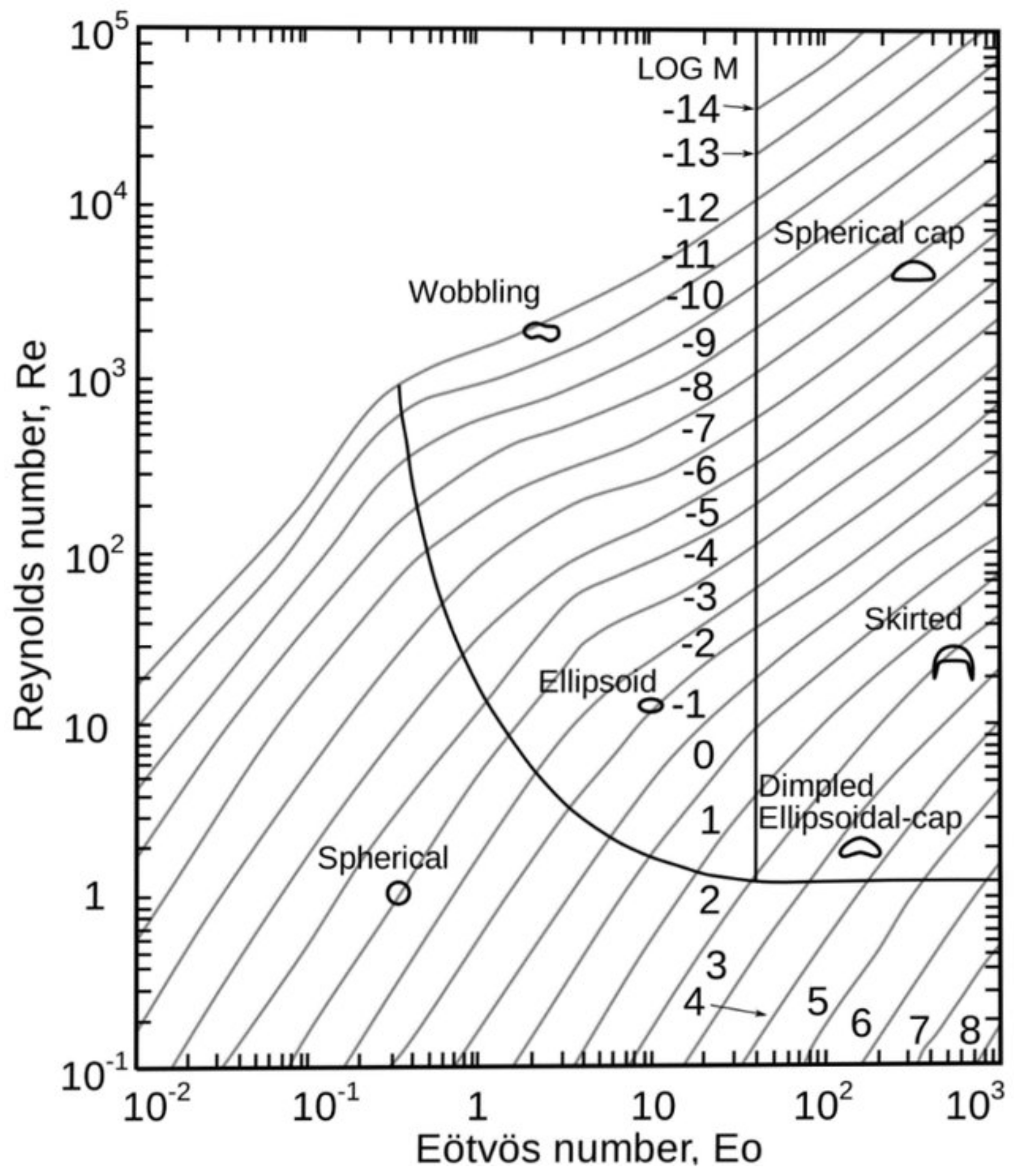
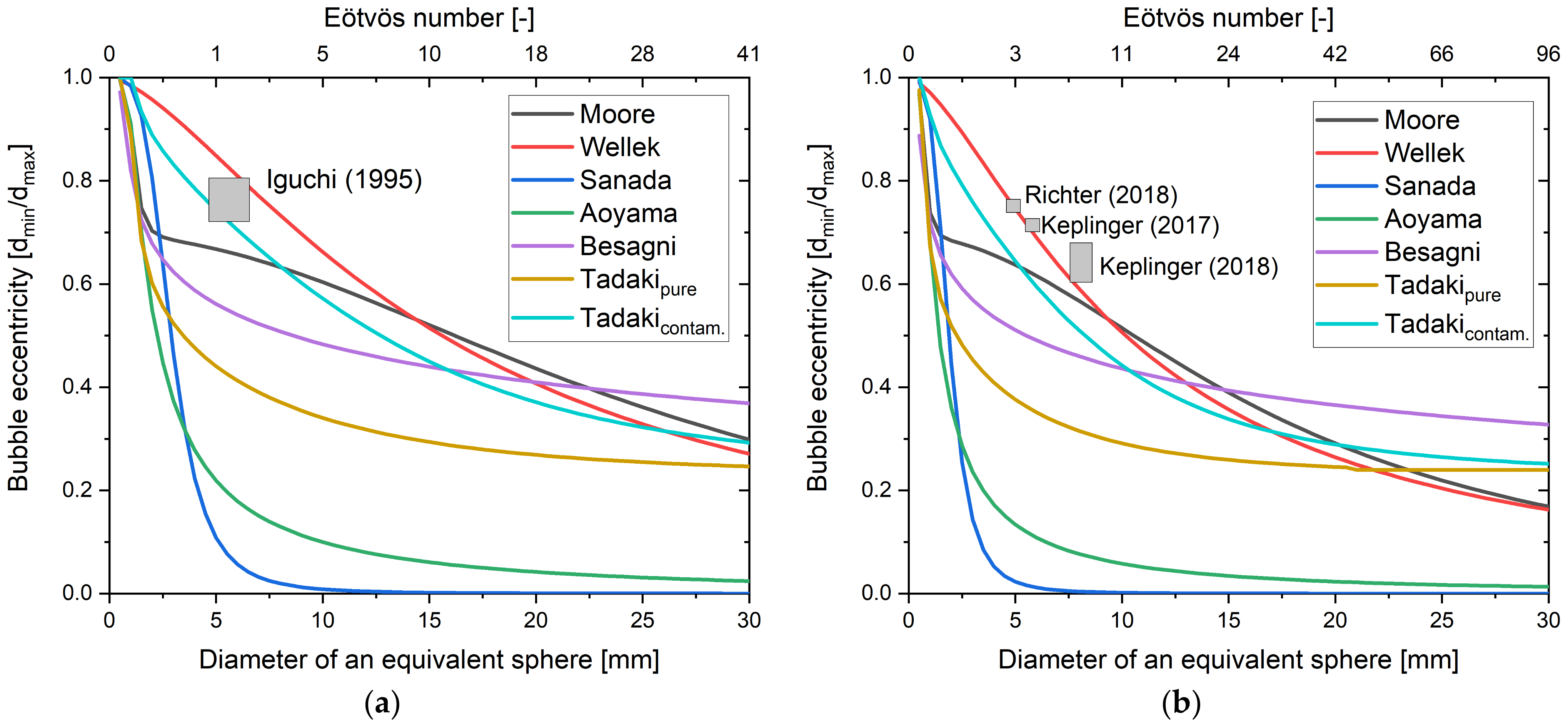
4. Bubble Deformation

In contrast to solid particles, droplet and bubble’s phase boundary may deform due to local pressure gradients. This leads to a complex interaction between the phase boundary and the surrounding flow. Bubble deformation influences the interfacial forces and heat and mass transfer, and vice versa. For the drag force, the deformation is usually considered implicitly in the drag coefficient though some exceptions exists (e.g., [78,79]). For the modelling of the lift force, the bubble shape has to be considered explicitly by the modified Eötvös number as discussed below.

An overview on different bubble shapes is provided in Figure 5. For small bubbles, the surface tension dominates, and the bubbles are of spherical shape (a). For medium-sized bubbles, the surface tension, viscous friction, and the inertia of the surrounding fluid are relevant for the bubble’s shape. If there is a relative velocity between bubble and fluid, the flow stops at the front stagnation point and the pressure increases towards the inside of the bubble. The surrounding streamlines bend to form a curve around the bubble. Due to the incompressibility of the fluid, an acceleration along the streamline must therefore take place, which reduces the local pressure. This effect results in the formation of an ellipsoidal bubble (b). At even higher relative velocities, cap or mushroom bubbles (c) are formed, which are caused by vortices in the wake behind the bubble [80]. Subsequently, the discussion is limited to spherical and ellipsoidal bubbles, largely omitting cap bubbles since the influence of deformation on the interfacial forces is assumed to be less pronounced for that case.

The deformation of ellipsoidal bubbles is usually described by either the eccentricity E or the shape factor φ given by Equation (23). In the stationary shape, oscillation is usually not considered, except for some measurements that concentrate on the interaction between wake, shape, and path oscillation.

$$\begin{gathered} \mathrm{Eccentricity} \mathrm{E}=\frac{{\mathrm{d}}_{\min }}{{\mathrm{d}}_{\max }} \\ \mathrm{Shape} \mathrm{factor} \mathsf{\phi }=\frac{{\mathrm{d}}_{\mathrm{eq}}}{{\mathrm{d}}_{\max }}{=\mathrm{E}}^{1/3} \end{gathered}$$

(23)

where the equivalent diameter, d_eq, is defined as the diameter of a sphere with the same volume as the distorted bubble. A simplified analytical solution for inviscid flows was derived by Moore [78] by balancing the normal stresses caused by dynamic pressure and surface tension at the stagnation points and on the equatorial plane. This analysis yields:

$$\mathrm{E}=\frac{1}{1+\frac{9}{64}\mathrm{We}+\mathrm{O}({\mathrm{We}}^2)}$$

(24)

The third term (O notification) indicates that this theory losses validity for higher Weber numbers, that is to say for stronger deviation from the spherical shape. Thus, this theory is only applicable for the limited range of slightly distorted ellipsoid bubbles in pure liquids. Therefore, dimensionless numbers describing the system are derived and coefficients for different f-functions (hypothesis) are established by fitting experimental datasets. Wellek et al. [81] discussed that a droplet’s shape depends on eight parameters: Density and viscosity of the gas and the surrounding fluid, the volume equivalent bubble diameter, surface tension, gravity, and the relative bubble velocity in steady state. By dimensional analysis, they derived five dimensionless numbers:

$$\mathrm{E}=\mathrm{f}\left(\frac{{\mathrm{d}}_{\mathrm{eq}}{\mathrm{u}}^2{\mathsf{\rho }}_{\mathrm{l}}}{\mathsf{\sigma }}, \frac{{\mathrm{d}}_{\mathrm{eq}}{\mathrm{u}\mathsf{\rho }}_{\mathrm{l}}}{{\mathsf{\mu }}_{\mathrm{l}}},\frac{\left({\mathsf{\rho }}_{\mathrm{l}}-{\mathsf{\rho }}_{\mathrm{g}}\right){\mathrm{gd}}_{\mathrm{eq}}^2}{\mathsf{\sigma }},\frac{{\mathrm{u}}^2}{{\mathrm{gd}}_{\mathrm{eq}}},\frac{{\mathsf{\mu }}_{\mathrm{l}}}{{\mathsf{\mu }}_{\mathrm{g}}}\right)=\mathrm{f}(\mathrm{We},\mathrm{Re},\mathrm{Eo},\mathrm{Fr},{\mathrm{N}}_{\mathsf{\mu }\mathrm{r}})$$

(25)

Haberman and Morton (1953) found the same parameters for bubbles, though they derived the drag coefficient c_D, the bubble Reynolds number, the Morton number, the Reynolds number inside the bubble, and the density ratio as dimensionless groups. If the density and viscosity of the gas is considered to be negligible, the number of dimensionless groups can be further reduced to three. Nowadays the bubble Reynolds number, Eötvös number, and Morton number are commonly used, although some correlations have been derived for the Weber number.

Grace et al. (original publication in French, found in [82]) presented the bubble shape as a function of these three dimensional groups in a diagram (Figure 6), often named the Grace diagram. This allows a qualitative estimate of the bubble shape. It can be seen that the deformation increases with increasing Eötvös and Reynolds number and decreasing Morton number. Furthermore, some shapes may only be present in certain Morton number ranges, although it should be mentioned that the boundaries are less strict in reality than shown in the diagram. Using neutron radiography in lead bismuth (log₁₀(Mo)~−13), Mishima et al. [28] found a good qualitative agreement between the predicted and observed bubble shapes.

Quantitative estimates are obtained by regression analysis of experimental data, mostly from experiments with single bubbles. Different f-functions exists. Wellek et al. [81] proposed:

$$\frac{1}{\mathrm{E}}{=1+\mathsf{\alpha }}_0{\displaystyle \prod }_{\mathrm{i}=1}^{{\mathrm{n}}_{\mathrm{tot}}}{\mathsf{\theta }}_{\mathrm{i}}^{{\mathsf{\alpha }}_{\mathrm{i}}}$$

(26)

where θ is a dimensionless group and α are the regression coefficients. A more complex f-function was proposed by Aoyama et al. [83]:

$$\frac{1}{\mathrm{E}}={\left[{1+\mathsf{\alpha }}_0{\displaystyle \prod }_{\mathrm{i}=1}^{{\mathrm{n}}_{\mathrm{tot}}}{\mathsf{\theta }}_{\mathrm{i}}^{{\mathsf{\alpha }}_{\mathrm{i}}}\right]}^{{\mathsf{\alpha }}_{\exp }}$$

(27)

Equation (26) might miss some higher-order correlations between the dimensionless groups while Equation (27) has a stronger tendency to overfit the experimental data.

Using Equation (26), Wellek et al. [81] correlated:

$$\mathrm{E}=\frac{1}{1+0.163{\mathrm{Eo}}^{0.757}}$$

(28)

Equation (28) was originally derived for liquid droplets, but it is now widely accepted that it also applies to contaminated bubbles [84]. For super purified fluids, Sanada et al. [5] used the same approach but correlated:

$$\mathrm{E}=\frac{1}{1+6.5{\mathrm{Eo}}^{1.925}}$$

(29)

This shows that the deformation is significantly reduced by contaminants. However, it should be mentioned that the measurements of Sanada et al. [5] were limited to small bubbles.

Correlations that only consider the Eötvös number have a limited ability to generalize. For instance, Wellek et al. [81] showed that Equation (28) is only applicable in a limited range of Morton numbers and is inaccurate for high viscous systems. They proposed that, instead, a correlation with the Weber number, similar to the analytical solution of the Moore (Equation (24)), should be used to cover a broader range of fluid properties. Similar results were found by Besagni and Deen [84]. Furthermore, the Eötvös number does not capture all dynamic effects of the hydrodynamic system, as shown in different studies. For example, Tomiyama et al. [85] observed an influence of the bubble release mechanism on the deformation, which cannot be captured by the Eötvös number. On the other hand, the Eötvös number is independent of the relative velocity, which makes it easily applicable in bubble swarms.

Tadaki and Maeda (1961, original publication in Japanese, found in [82]) experimentally found a dependency on the Reynolds and Morton number, which was later termed the Tadaki number Ta:

$$\mathrm{Ta}={\mathrm{ReMo}}^{0.23}$$

(30)

For bubble deformation, expressed by the shape factor φ, they derived:

$$\mathsf{\phi }={\mathrm{E}}^{\frac{1}{3}}=\begin{array}{cc}1& \mathrm{Ta} < 2 \left(\mathrm{spherical}\right)\\ 1.14{\mathrm{Ta}}^{-0.176}& 2 < \mathrm{Ta} < 6 \left(\mathrm{ellipsoid}\right)\\ 1.36{\mathrm{Ta}}^{-0.28}& 6 < \mathrm{Ta} < 16.5 \left(\mathrm{ellipsoid}\right)\\ 0.62& 16.5 < \mathrm{Ta} \left(\mathrm{spherical} \mathrm{cap}\right)\end{array}$$

(31)

Fan and Tsuchiya [80] compared this correlation with literature data for purified liquids and determined that it is applicable for contaminated fluids. They generalized an existing correlation by Vakhrushev and Efremov [86] to be used for pure and contaminated liquids:

$$\frac{1}{\mathrm{E}}=\begin{array}{cc}1& \mathrm{Ta} \le {\mathrm{Ta}}_1\\ \{{\mathrm{c}}_1+{\mathrm{c}}_2\tanh [{\mathrm{c}}_3({\mathrm{c}}_4 - \log (\mathrm{Ta})]{\}}^{\mathrm{m}}& {\mathrm{Ta}}_1 \le \mathrm{Ta} \le {\mathrm{Ta}}_2\\ {(\mathrm{h}/\mathrm{b})}_{\mathrm{cap}}& {\mathrm{Ta}}_2 \le \mathrm{Ta}\end{array}$$

(32)

The fitting parameters of this correlation are summarized in

Table 3. Parameters for Equation (32) from Vakhrushev and Efremov [86] and Fan and Tsuchiya [80].

System	m	(h/b)cap	Ta1	Ta2	c1	c2	c3	c4
3Dcontaminated	3	0.24	1	40	0.81	0.2	2.0	0.8
3Dpure	3	0.24	0.3	20	0.81	0.2	1.8	0.4

.

Aoyama et al. [87] used a more complex f-function given in Equation (27) and found a correlation that takes the bubble Reynolds and Eötvös numbers into account.

$$\mathrm{E}=\frac{1}{{\left[1+0.016{\mathrm{Eo}}^{1.12}\mathrm{Re}\right]}^{0.388}}$$

(33)

All correlations presented up to this point have common ground in the fact that they are based on measurements of single bubbles in stagnant liquids. However, it is likely that bubble deformation is affected by the presence of other bubbles in a bubble swarm. This subject was investigated by Ziegenhein and Lucas [88] using data from six different experimental setups with pure water. The dataset included experiments with single bubbles in linear shear flows and different bubble columns. Because not all instantaneous local quantities could be measured simultaneously, averaged values for the turbulence, dynamic pressure, and bulk flow field were used. Their measurements showed that deformation is largely independent of the flow rate, i.e., void fraction and fluid flow. The deformation found in single bubble experiments were less pronounced than in bubble swarms, but the difference is generally small. For smaller Eötvös numbers, this difference is more pronounced than for larger Eötvös numbers. A comparison with existing correlations showed that none of them reflect the data well over the whole range of values. For small Eötvös numbers, there is a good agreement with measurements in super purified liquids by Sanada et al. (Equation (29)) [5]. For larger Eötvös numbers, however, this correlation clearly overestimates the deformation. Compared with Tadaki number correlations, there is good agreement with the correlation of Fan and Tsuchiya (Equation (32) and Table 3 up to Ta < 3. Beyond that, significantly less deformation was found. From these results, the authors concluded that for a final evaluation of bubble deformation in swarms, the local flow conditions would have to be considered, which is currently not possible. For larger bubbles, however, there are very similar tendencies as in experiments with single bubbles.

Figure 6. Grace diagram to approximate the bubble shape as a function of the Eötvös, Reynolds, and Morton number (original in French, reproduced from [88], with permission from Elsevier, 2021).

Figure 6. Grace diagram to approximate the bubble shape as a function of the Eötvös, Reynolds, and Morton number (original in French, reproduced from [88], with permission from Elsevier, 2021).

Besagni and Deen [84] evaluated a large dataset of measurements in pure and contaminated systems for single bubbles and swarms, ranging from −10.8 < log₁₀(Mo) < 2.3, which was collected by different researchers. Using Equation (27) as f-function, they correlated:

$$\mathrm{E}=\frac{1}{{\left[1+0.4{\mathrm{Eo}}^{1.19}{\mathrm{Re}}^{1.05}\right]}^{0.07}} \approx \frac{1}{{\left[1+0.45\mathrm{EoRe}\right]}^{0.08}}$$

(34)

In addition, they compared existing correlations with their data and showed than none of them could predict the eccentricity very well in a wide range of conditions. This result indicates that a comprehensive prediction of the bubble deformation is still difficult. Though a large number of correlations have been proposed, none seems to be applicable for all experimental conditions. There are different reasons for that. First, the dimensionless numbers are on different scales. While Morton numbers are usually very small, the Reynolds number is usually some order of magnitudes larger. Feature scaling should be applied before fitting an f-function to avoid any scale effects. More importantly, all measurements suffer from a systematic bias by contaminants. Measurements by Sanada et al. [5] showed that even smallest amounts of organic substances, which cannot be avoided experimentally, have significant influence of the bubble rising behavior and its deformation. Since the purity of the investigated systems is usually provided qualitatively, the bias of contamination results in different measurement uncertainties. Finally, one has to bear in mind that the approximation of a symmetric ellipsoid becomes rather inaccurate for larger bubbles, particular in low Morton number systems and that shape oscillation is usually neglected. Thus, the experimental data, in particular for larger bubbles, scatter significantly. Even more difficult is the extrapolation of existing correlations to liquid metals. Iguchi et al. [24] developed a multi-needle resistivity probe to reconstruct the shape of gas bubbles. A cap or mushroom shape was found for approximately 25 mm bubbles in Wood’s metal. A correlation was found between the averaged bubble Reynolds number (mean bubble size and velocity as characteristic length and velocity, respectively) and the modified Weber number (multiplied by the density ratio) [23]. However, the measurements were made just above the injector, so that a strong influence of the initial deformation due to the tearing off of the bubble can be assumed. There are very few studies investigating the deformation of gas bubbles in liquid metals quantitatively [22,26,27,31]. These studies are all based on X-ray measurements, which can be used to visualize the bubble. However, the deformation is only explicitly stated by Richter et al. [31] and Keplinger et al. [27]. For the other studies, the deformation must be roughly estimated from the published images. A comparison of the presented correlation with the measured values in liquid steel and GaInSn is shown in Figure 7. The bubble Reynolds number and Weber number were estimated for this purpose with the drag coefficient according to Dijkhuizen et al. [89] (Equation (45)). The physical properties employed for this estimate are listed in

Table 4. Physical properties of the investigated liquid metals.

Fluid	Density [kg/m3]	Viscosity [Ns/m2]	Surface Tension [N/m]	log10 (Mo)
GaInSn	6330	0.00234	0.585	−12.6
Steel	6900	0.00506	1.5	−12.6
Mercury	13,550	0.00155	0.487	−13.4
Silver	9510	0.00389	0.92	−12.5

.

It can be seen that most correlations significantly overestimate the deformation. However, there is good agreement with the model of Wellek et al. [81]. This is surprising, since this model is only valid for contaminated bubbles in aqueous systems. It is not clear whether the lower deformation can be explained by the presence of contaminants or by the significantly higher surface tension of the liquid metals. A general problem of the used X-ray measurements is, however, that only the contour of the bubble is visible. Thus, it is difficult to distinguish between ellipsoids and spherical cap bubbles [24]. In addition, the high absorption of the liquid metals conditions that very narrow experimental setups have to be used. It is therefore quite possible that the proximity to the wall has an influence on the deformation. Numerically, the deformation of argon bubbles in steel was qualitatively investigated by Xu et al. [90] and Wang et al. [91]. Both use the volume of fluid surface tracking method. They reported that bubbles are spherical after injection but become wobbly (d_b ≤ 7 mm) or ellipsoidal cap shaped (d_b > 7 mm), depending on their size and their Eötvös and Reynolds numbers. However, when evaluating these results, it should be noted that no turbulence model was used in both studies, but the mesh resolution used is too coarse for a real DNS. Therefore, the models can be classified as implicit large eddy turbulence model (LES) without a subgrid model, which underestimates the draining effect of the small-scale eddies on the energy cascade. Therefore, it is likely that the resolved turbulence is overestimated in both studies, which certainly has some influence on the bubble shape.

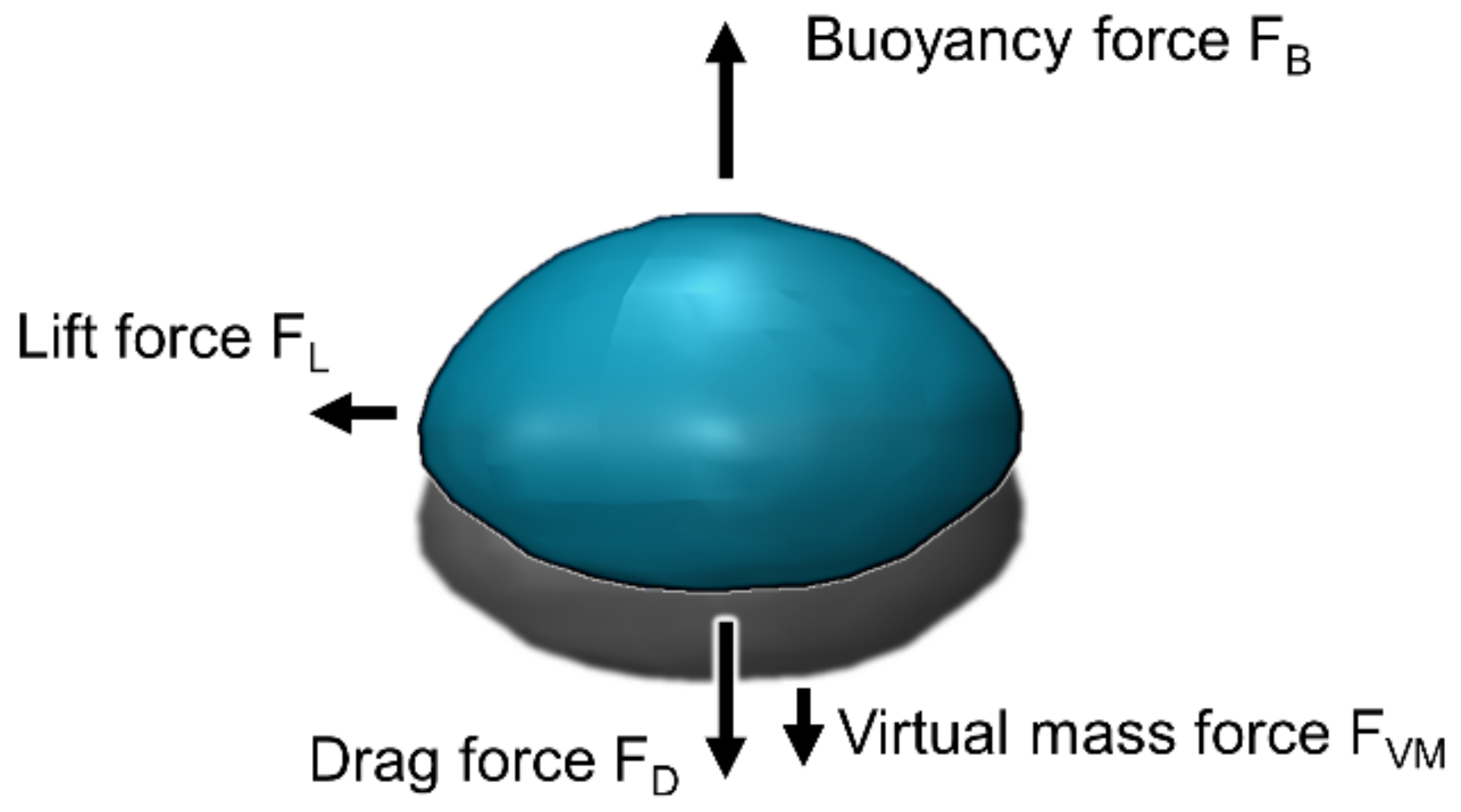
5. Interfacial Force Closure

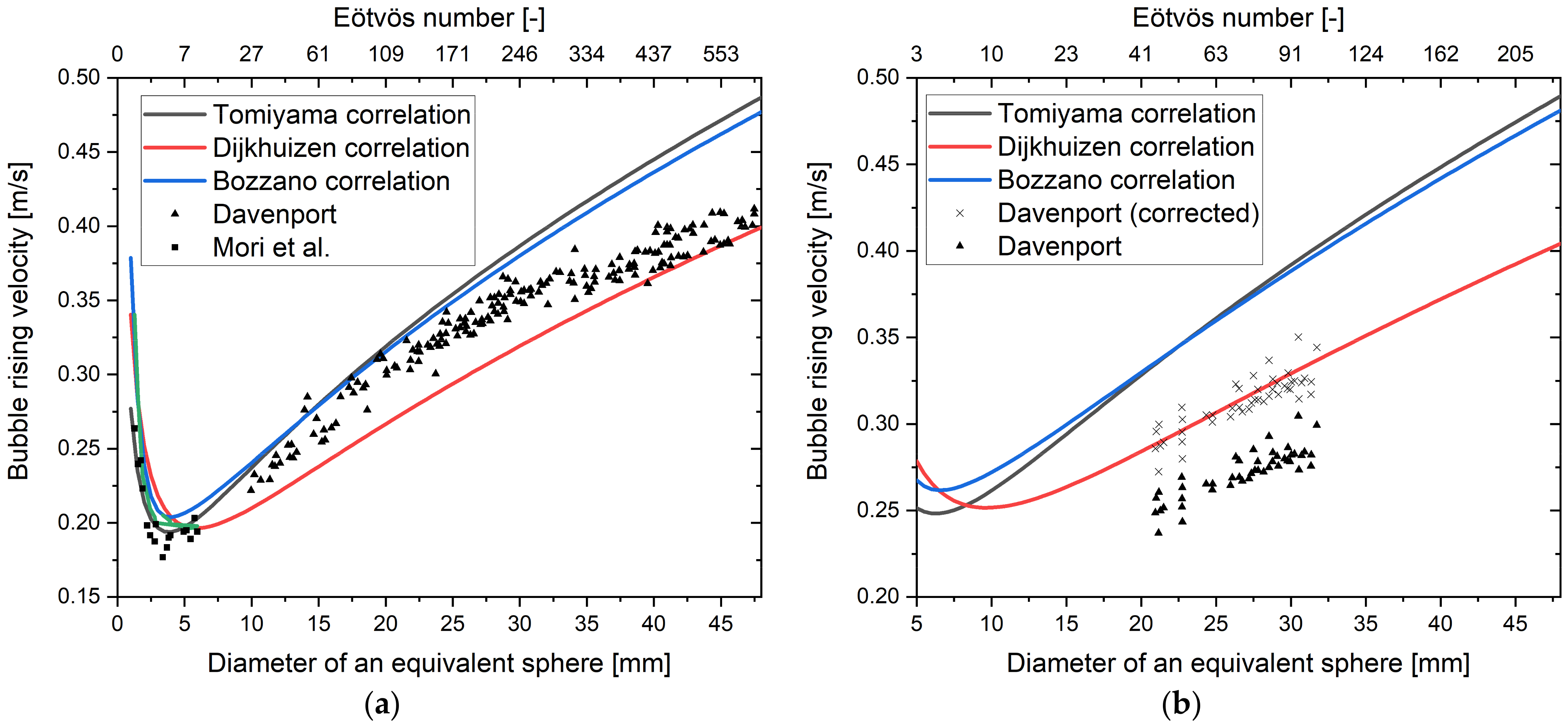
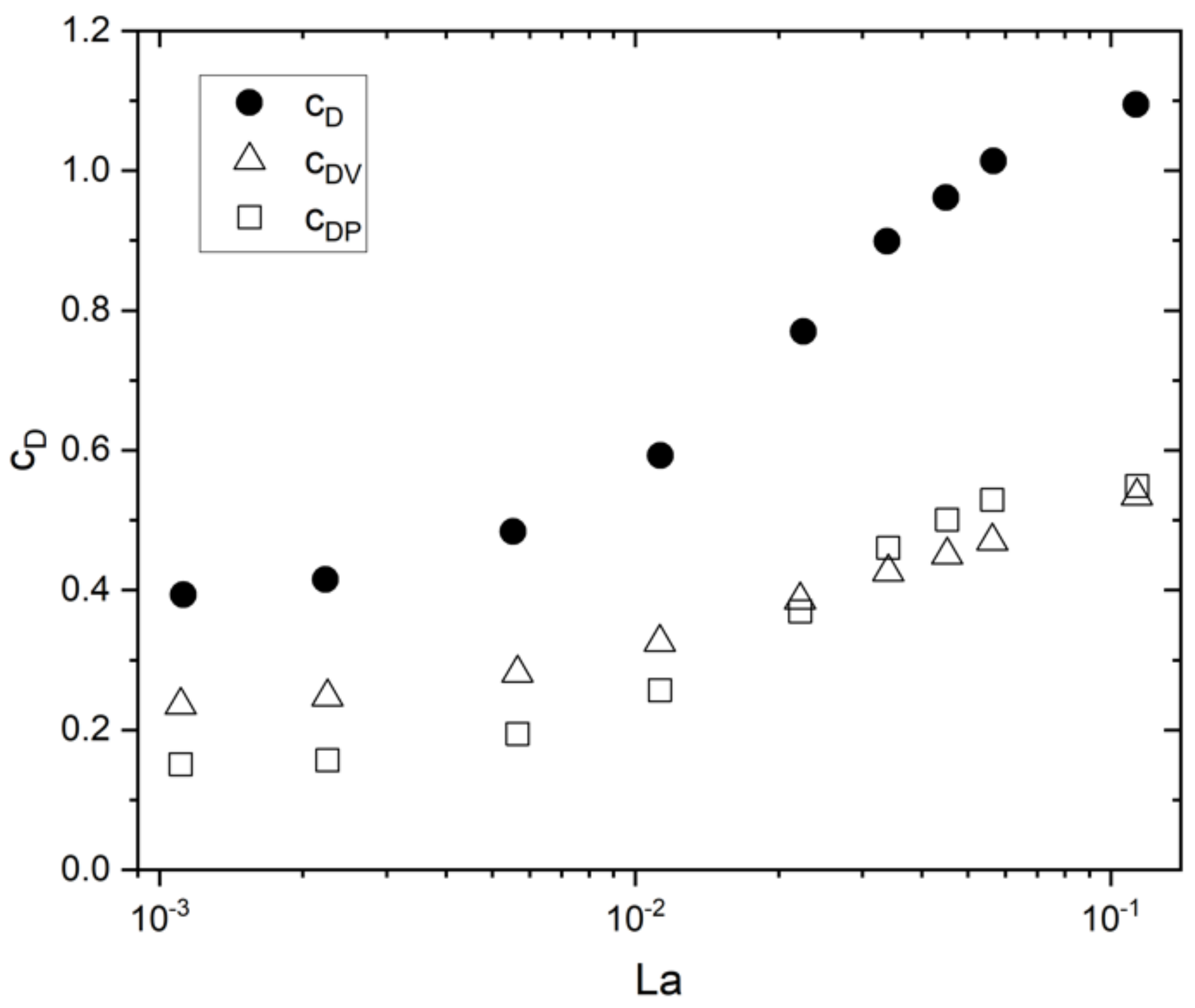
According to the second Newtonian axiom, the acceleration of bubbles and thus their motion can be described by the sum of all forces acting on them. For bubbles, the buoyancy, the drag, the lift, and the virtual mass force are decisive. Thus, the velocity of a bubble is governed by:

$$\frac{\partial {\mathrm{u}}_{\mathrm{b}}}{\partial \mathrm{t}}=\frac{1}{{\mathrm{m}}_{\mathrm{b}}}{{\displaystyle \sum }}_{\mathrm{i}}{\mathrm{F}}_{\mathrm{i}}{=\mathrm{gV}}_{\mathrm{b}}\left({\mathsf{\rho }}_{\mathrm{l}}-{\mathsf{\rho }}_{\mathrm{b}}\right)+{\mathrm{F}}_{\mathrm{D}}+{\mathrm{F}}_{\mathrm{L}}+{\mathrm{F}}_{\mathrm{VM}}$$

(35)

Subsequently, the different forces, shown in Figure 8, are discussed, and existing correlations are critically analyzed with regard to their application to liquid metals.

5.1. Drag Force

The drag force determines the bubble’s rising velocity and contributes the main part of the momentum transfer from bubbles to liquid. It arises through a relative velocity between the bubble and the continuous phase. It comprises two phenomena, a viscous friction force and a force caused by a pressure gradient along the bubble surface in the direction of movement. The local pressure gradient is the result of the bubble wake and is therefore more pronounced in the case of high bubble Reynolds numbers. The drag force is determined by:

$${\mathrm{F}}_{\mathrm{D}}=\frac{1}{2}{\mathrm{c}}_{\mathrm{D}}{\mathsf{\rho }}_{\mathrm{l}}\frac{{\mathsf{\pi }\mathrm{d}}_{\mathrm{b}}^2}{4}{\left({\mathrm{u}}_{\mathrm{b}}-{\mathrm{u}}_{\mathrm{l}}\right)}^2$$

(36)

Equation (34) indicates, that the drag force is directly proportional to the dimensionless drag coefficient c_D, which depends on bubble properties and the flow conditions. The effect of bubble deformation is usually lumped into c_D as well. By dimensionless analysis, it can be shown that the drag coefficient depend on the bubble Reynolds number, the Eötvös number, and the Morton number [82].

Analytically, Levich (in [92]) derived inviscid flows, for which the influence of viscous friction can be neglected:

$${\mathrm{c}}_{\mathrm{D}}=\frac{48}{\mathrm{Re}}$$

(37)

For creeping flows, for which the pressure contribution by the wake is negligible, Hadamard (in [82]) derived:

$${\mathrm{c}}_{\mathrm{D}}=\frac{16}{\mathrm{Re}}$$

(38)

Mei and Klausner [93] proposed an analytical approximation for spherical bubbles at arbitrary Reynolds numbers, which fits Equations (37) and (38) asymptotically.

$${\mathrm{c}}_{\mathrm{D}}=\frac{16}{\mathrm{Re}}\left[1+{\left(\frac{8}{\mathrm{Re}}+\frac{1}{2}\left(1+3.315{\mathrm{Re}}^{-0.5}\right)\right)}^{-1}\right]$$

(39)

These analytical solutions are often used as benchmark for experimental or numerical approximations of c_D. However, they are not applicable for most industrial processes, since the bubbles are usually deformed and the fluid system is contaminated to some extent, which increase the real drag coefficient.

The second and most common approach to derive c_D are experimental measurements. Usually, the rise of single bubbles in stagnant (u_l = 0), mostly aqueous liquids, is studied. After the bubble reaches its terminal rising velocity, the drag force is in equilibrium with the buoyancy force. The drag coefficient is then given by:

$${\mathrm{c}}_{\mathrm{D}}=\frac{4}{3}\frac{\left({\mathsf{\rho }}_{\mathrm{l}}-{\mathsf{\rho }}_{\mathrm{b}}\right){\mathrm{d}}_{\mathrm{b}}\mathrm{g}}{{\mathsf{\rho }}_{\mathrm{l}}{\mathrm{u}}_{\mathrm{b}}^2}$$

(40)

A large number of correlations based on this approach can be found in the literature. These are listed for example by Clift et al. [82] or Pang and Wei [94]. Here, only some correlations, which were found in close agreement with validation data in CFD studies, are repeated.

By reviewing existing correlations, Tomiyama et al. [95] derived three correlations in dependence on the degree of contamination of the system. For pure liquids, they derived:

$${\mathrm{c}}_{\mathrm{D}}=\max \left[\min \left[\frac{16}{\mathrm{Re}}\left(1+0.15{\mathrm{Re}}^{0.687}\right),\frac{48}{\mathrm{Re}}\right], \frac{8}{3}\frac{\mathrm{Eo}}{\mathrm{Eo}+4}\right]$$

(41)

This correlation is often employed in numerical models. For example, Frank et al. [96] showed that this correlation has the best accordance with experimental validation data. Bröder and Sommerfeld [7] proved its validity by experimental measurements in (dilute) bubble swarms.

An entirely different approach to correlate the drag coefficient was proposed by Bozzano and Dente [79]. Because the bubble deformation and the wake structure are correlated, they argued that the drag may be described by the bubble deformation, which is usually implicitly considered:

$${\mathrm{c}}_{\mathrm{D}}=\mathrm{f}{\left(\frac{\mathrm{a}}{{\mathrm{R}}_{\mathrm{eq}}}\right)}^2$$

(42)

where f is a friction factor given by:

$$\mathrm{f}=\frac{48}{\mathrm{Re}}\left(\frac{1+12{\mathrm{Mo}}^{0.33}}{1+36{\mathrm{Mo}}^{0.33}}\right)+0.9\frac{{\mathrm{Eo}}^{1.5}}{1.4\left(1+30{\mathrm{Mo}}^{0.167}\right)+{\mathrm{Eo}}^{1.5}}$$

(43)

The second term on the right hand side is a deformation factor given by:

$$\mathrm{DEF}={\left(\frac{2\mathrm{a}}{{\mathrm{d}}_{\mathrm{eq}}}\right)}^2\cong \frac{10\left(1+1.3{\mathrm{Mo}}^{0.167}\right)+3.1\mathrm{Eo}}{10\left(1+1.3{\mathrm{Mo}}^{0.167}\right)+\mathrm{Eo}}$$

(44)

However, experimental measurements have the disadvantage that it is very difficult to control all boundary conditions exactly. In particular, contaminants have a significant influence on the rising velocity as discussed in detail below.

A correlation for c_D, based on a DNS, was proposed by Dijkhuizen et al. [89]:

$${\mathrm{c}}_{\mathrm{D}}=\sqrt{{\mathrm{c}}_{\mathrm{D}}{\left(\mathrm{Re}\right)}^2{+\mathrm{c}}_{\mathrm{D}}{\left(\mathrm{Eo}\right)}^2}$$

(45)

where c_D(Re) is the analytical solution by Mei and Klausner (Equation (39)) and c_D(Eo) is given by:

$${\mathrm{c}}_{\mathrm{D}}\left(\mathrm{Eo}\right)=\frac{4\mathrm{Eo}}{\mathrm{Eo}+9.5}$$

(46)

A comparison of the different drag correlations independent of the Eötvös number and the bubble equivalent diameter is provided in Figure 9. The physical properties of the liquid metals employed for this comparison are listed in Table 4. It can be seen that Equation (45) predicts higher rising velocities and lower drag coefficients, respectively, compared to Equations (41) and (42), indicating that the experimental correlations might be influenced by contaminants.

Those correlations show that the drag force at low Reynolds numbers is governed by the Reynolds number, but at sufficiently high Reynolds numbers, it is determined by the Eötvös number. Though some correlations explicitly include the Morton number [79,97], most studies agree that the Reynolds, Eötvös, and Morton numbers depend on one another when considering the drag force [95]. Thus, the system is fully described by the Reynolds and Eötvös number. However, it should be noted that almost all measurements were performed in aqueous systems where the density difference between fluid and bubble and the surface tension can be varied only to a small extent. Due to measurement difficulties in liquid metals, data from this fluid systems are very scarce. Usually, bubble chains were investigated, which has the disadvantage that the assumption of a stagnant fluid cannot be made. Thus, the bubble rising velocity is different from the relative velocity and a drag coefficient cannot be derived. There are only a few exceptions such as the measurements by Davenport [19], Mori et al. [98], Zhang et al. [99], and Wang et al. [32]. Davenport [19] performed measurements in mercury at room temperature and in liquid silver at 1000 °C. Bubbles were generated by a rotating cup. This cup initially pointed downwards, so that gas flowing in was collected in it. When the cup was turned, the collected gas rose as a single bubble. The rising velocity was derived by dividing the rising path by the time between bubble release and bubble’s breaking through the bath surface. Mori et al. [98] measured the rising velocity by electric conductivity probes. Zhang et al. [99] and Wang et al. [32] both employed ultrasonic doppler velocimetry. A comparison between the different drag correlations described above and the measurements is provided in Figure 9. For mercury (Figure 9a), the measured rising velocities of small bubbles are slightly lower than predicted, but generally agree very well with the correlations. For larger bubbles, the experimental values lie between the predicted values by Tomiyama et al. [95] (Equation (41)) and Bozzano and Dente [79] (Equation (42)) and the numerical correlation by Dijkhuizen et al. [89] (Equation (45)). A possible explanation might be a slight contamination of the used mercury or the measurement uncertainty. Unfortunately, information about the purity of the mercury is neither provided by Davenport [19] nor by Mori et al. [98]. For intermediate Eötvös numbers, the measurements are in better accordance with the experimentally derived correlations, while for higher Eötvös numbers, they fit the numerically derived correlation better.

For liquid silver (Figure 9b), two measurement methods were used by Davenport [19], depending on whether the bubble’s acceleration phase was taken into account or not. With the latter method (marked with an x), about 15% higher rising velocities were derived. This leads to an excellent agreement with the Dijkhuizen et al. [89] (Equation (45)) correlation. Again, no remark on the purity of the liquid silver was given. In GaInSn (Figure 9c), where measurements were made at relatively small Eötvös numbers, both authors found slightly lower rising velocities than predicted for pure systems. This could be an indication that contaminants influence the rising velocities.

Figure 9. Comparison of drag models with measured bubble rising velocities in mercury (a), silver (b), and GaInSn (c) [19,32,98,99].

Figure 9. Comparison of drag models with measured bubble rising velocities in mercury (a), silver (b), and GaInSn (c) [19,32,98,99].

In addition, the bubble rising velocity of single bubbles in liquid steel was investigated numerically [90,91]. A comparison of the results with the correlations is shown in Figure 10. As with the experimental measurements, there is fairly good agreement with the correlations. However, no distinct tendency to which correlation fits better can be derived. As with the bubble deformation, however, it should be noted that the resolution of the numerical grid used was too coarse for a real DNS.

Nevertheless, the comparison can be seen as an indication that the correlations derived from aqueous systems can be extrapolated to liquid metals. For small Eötvös numbers, there is a small uncertainty due to the influence of contaminants. For larger Eötvös numbers, the correlations are based on relatively few data, so there may be another uncertainty due to extrapolation of the correlations. For a final conclusion regarding which correlation should be used for molten metals, no conclusion can be drawn by now since the verification dataset is too small and its measurement uncertainty is too high. The same applies for the influence of contaminants in liquid metals.

5.1.1. Influence of Contaminants

Contaminants cause a reduction of the drag force due to the Marangoni effect or by a demobilization of the phase boundary. Because the viscosity of the fluid in the bubble is typically much smaller than that of the surrounding fluid, the boundary condition at the uncontaminated bubbles is typically a zero-shear-stress condition (Figure 11a). However, in contaminated systems, contaminants attached at the front of the bubble slide along the surface and accumulate at the bubble’s rear (Figure 11b). This leads to gradients in surface tension along the bubble surface, causing a tangential shear force [100]. At sufficiently high contamination, complete demobilization of the bubble’s surface occurs, and its flow condition changes from a no-shear to a no-slip condition (Figure 11c). This causes the bubbles to behave approximately like rigid particles.

Although this effect has been known for a long time, it is still not fully understood and can only be roughly quantified. A frequently employed approximation was derived by Tomiyama et al. [95]. Amongst a correlation for pure systems (Equation (41)), they derived correlations for slightly contaminated (Equation (47)) and fully contaminated (e.g., tap water) (Equation (48)) systems.

$${\mathrm{c}}_{\mathrm{D}}=\max \left[\min \left[\frac{24}{\mathrm{Re}}\left(1+0.15{\mathrm{Re}}^{0.687}\right),\frac{72}{\mathrm{Re}}\right], \frac{8}{3}\frac{\mathrm{Eo}}{\mathrm{Eo}+4}\right]$$

(47)

$${\mathrm{c}}_{\mathrm{D}}=\max \left[\frac{24}{\mathrm{Re}}\left(1+0.15{\mathrm{Re}}^{0.687}\right) , \frac{8}{3}\frac{\mathrm{Eo}}{\mathrm{Eo}+4}\right]$$

(48)

The different rising velocities derived from the three correlations are shown in Figure 12. It can be seen that, according to Tomiyama et al. [95], the contamination is only relevant for small bubbles.

However, a comparison with the correlation by Dijkhuizen et al. [89] (Equation (45)) suggest that the measurement for all three correlations are influenced by contaminants and that the rising velocity of larger bubbles is influenced as well. Indeed, the correlation for pure systems was derived from measurements in distilled water, which is far from being pure. Therefore, the question of whether contamination is important for all bubble sizes cannot yet be answered. Some authors argue that for large Eötvös and Weber numbers, surface tension no longer plays a role for c_D and thus contaminants also no longer have an influence on the rising velocity. However, contaminants not only affect the flow boundary condition at the bubble surface, but also the deformation and vortex shedding. Therefore, Tasoglu et al. [101] found that contaminants are relevant for a broad range of Eötvös numbers, but the effect is much more pronounced for smaller bubbles. A problem here is that DNS studies usually investigate very small Reynolds number flows and large Morton numbers, since the computational costs increases with Re^9/4. Experimental studies, on the other hand, face the problem that it is practically impossible to generate completely uncontaminated systems. Therefore, sound studies on the effect of contaminates for large bubbles at relevant Reynolds numbers are largely lacking. A further critique of the Tomiyama et al. [95] approach is that for most engineering applications, there is no a priori definition of the degree of contamination of the system.

There are numerous attempts to quantify the range of intermediate contamination more precisely. The results are summarized by the reviews of Cuenot et al. [102] and Takagi and Matsumoto [100]. For low contaminant concentrations, Zhang and Finch [103] showed that bubbles may rise a few meters until they reach their terminal velocity. In that case, the effect is governed by the Hatta number, Ha, which is the ratio of adsorption velocity to the bubble rising velocity:

$$\mathrm{Ha}=\frac{{\mathrm{kc}}_{\infty }{\mathrm{d}}_{\mathrm{b}}}{\left|{\mathrm{u}}_{\mathrm{d}}-{\mathrm{u}}_{\mathrm{l}}\right|}$$

(49)

Furthermore, the strength of the effect not only depends on the concentration of the contaminants, but also on the type of contaminants [104]. Thus, it was suggested that the effect should be quantified by the Langmuir number, La, which is defined as the ratio between the adsorption and desorption rate:

$$\mathrm{La}=\frac{{\mathrm{c}}_{\infty }}{\mathsf{\beta }}$$

(50)

The drag coefficient as a function of the Langmuir number is shown in Figure 13. It can be seen that the Langmuir number not only influences the viscous share of the drag force, but also the pressure share. It should be noted though that the results shown in Figure 13 were derived for low Re numbers. Thus, it is not clear whether the dependency of the pressure share on the Langmuir number can be extrapolated to higher Re numbers where the flow is mainly governed by inertia effects.

However, the relationships described above are still the subject of molecular dynamics research. They can hardly be used in engineering science, since information on concentrations and absorption and desorption kinetics is generally not available. This is particularly true for liquid metal systems. Therefore, it is not possible to determine whether contaminants, for example alloying elements, trace elements, or non-metallic inclusions, have an influence on bubble behavior in metallurgical processes.

5.1.2. Influence of Surrounding Bubbles

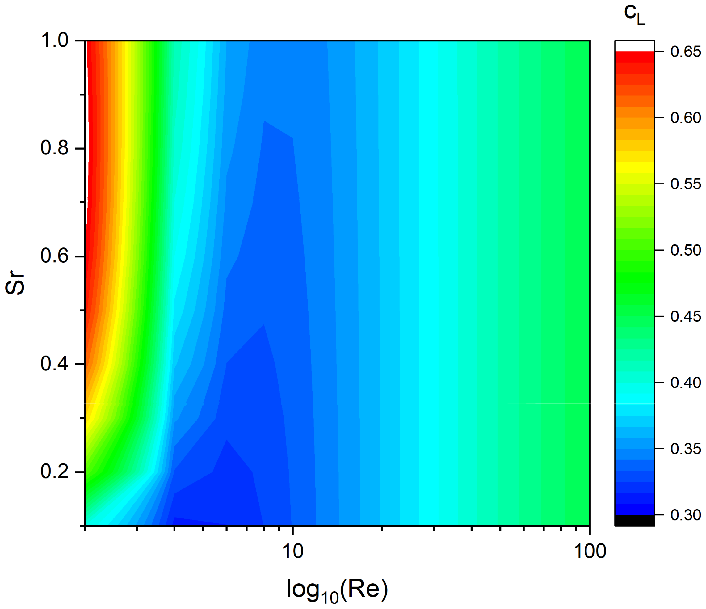
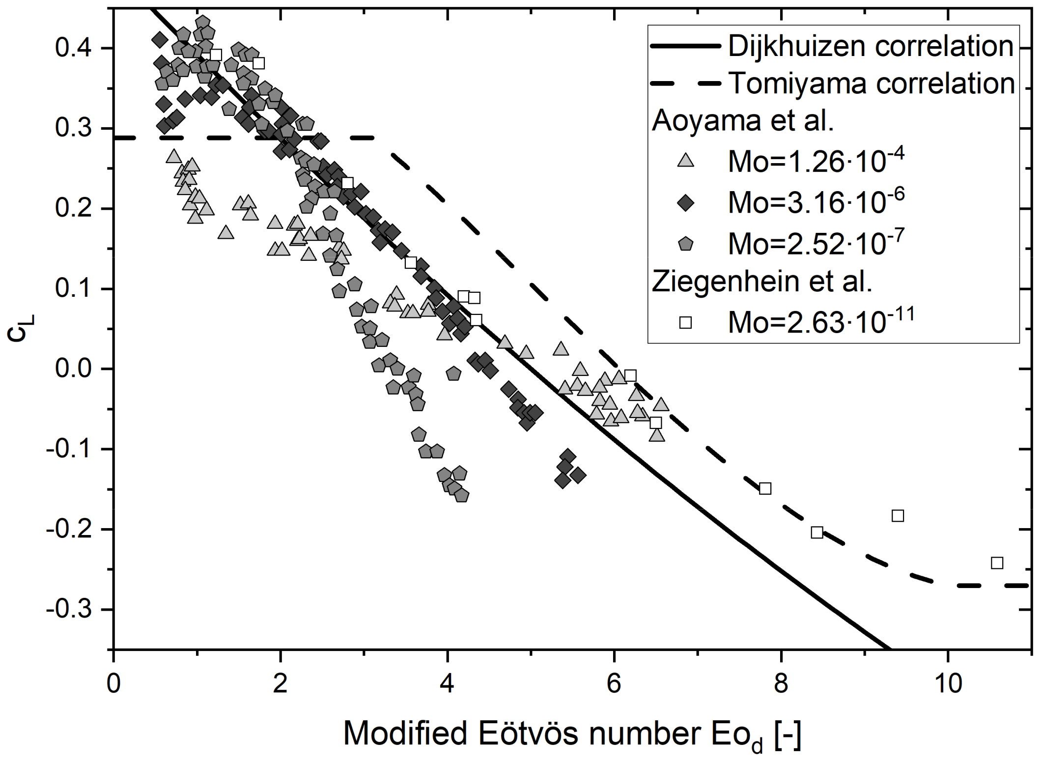
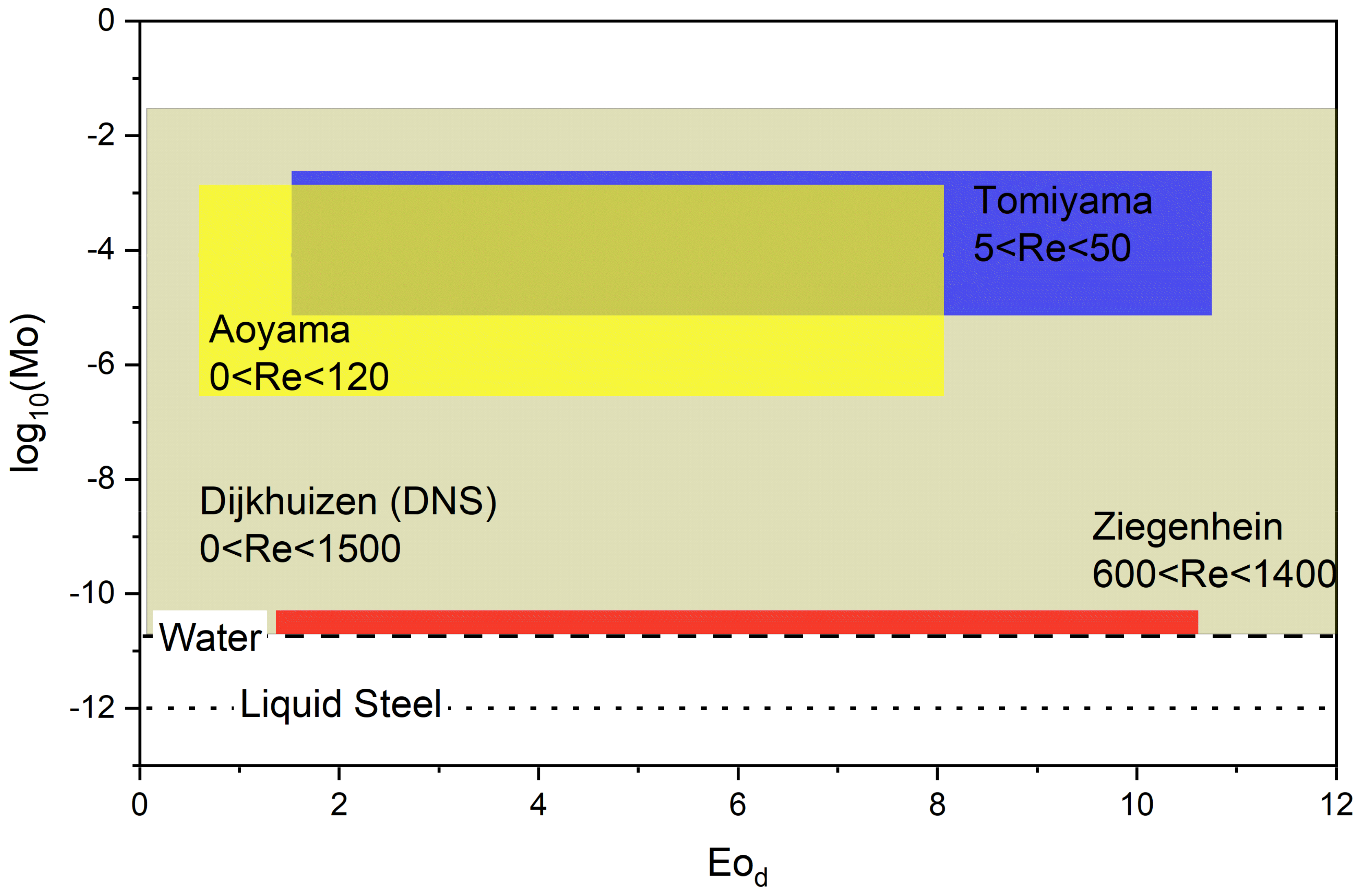
The studies and correlations presented so far all dealt with single bubbles in stagnant liquids. However, some authors, summarized by Simonnet et al. [106], showed that these correlations are no longer valid when the bubble is surrounded by other bubbles. A similar effect for the sedimentation of solid particles was found by Richardson and Zaki [107]. In particular, they found a correlation between the sedimentation velocity of single particles, the sedimentation velocity of particles in suspensions, and the suspension density (equivalent to the void fraction in bubbly flows):

$${\mathrm{u}}_{\mathrm{rel}, \mathrm{swarm}}={\mathrm{u}}_{\mathrm{rel}, \mathrm{single}}{\left(1 - {\mathsf{\alpha }}_{\mathrm{glob}}\right)}^{\mathrm{n}}$$

(51)

where the exponent n was coined Richardson and Zaki exponent by Simonnet et al. [106]. Because the particle velocity and the drag force are correlated, the effect of particle swarms on the drag force can be taken into account by multiplying a correction factor to the drag coefficient of single particles:

$${\mathrm{c}}_{\mathrm{D},\mathrm{swarm}}={\mathrm{c}}_{\mathrm{D},\mathrm{single}}·\mathrm{f}(\mathsf{\alpha },\dots )$$

(52)

Most early studies on bubble swarms used Equation (52) and fitted the Richardson and Zaki exponent to their experimental data [106]. However, in bubble swarms, the situation is more complex since the possible degree of freedom for bubbles is greater than those of solid particles. Thus, Lockett and Kirkpatrick [108] added an additional factor that takes into account bubble deformation.

These correlations used a global void fraction. However, Garnier et al. [109] argued that the change of drag is caused by local, not global, phenomena. Experimentally, the local void fraction was determined by the quotient of time in which a bubble was detected in the measurement probe and the total measurement time [110].

A correlation based on the local void fraction was established by Simonnet et al. [106]:

$$\mathrm{f}\left(\mathsf{\alpha }\right)=\left(1-{\mathsf{\alpha }}_{\mathrm{loc}}\right){\left[{\left(1-{\mathsf{\alpha }}_{\mathrm{loc}}\right)}^{\mathrm{m}}+{\left(4.8\frac{{\mathsf{\alpha }}_{\mathrm{loc}}}{1-{\mathsf{\alpha }}_{\mathrm{loc}}}\right)}^{\mathrm{m}}\right]}^{-\frac{2}{\mathrm{m}}}$$

(53)

where m is a smoothing parameter, estimated with a value of 25 by experimental data. Simonnet et al. [106] observed that the increase of the drag coefficient with increasing void fraction, which was reported by all previous studies, is only valid for small bubbles (d_b ≤ 7 mm). For larger bubbles, the drag increases up to a critical void fraction of approximately 15% and decreases afterwards. Thus, Equation (53) is only valid for an air–water system, where bubble diameters are between 5 and 10 mm, with the restriction that for void fractions above 15%, the bubble diameter has to be larger than 7 mm. Simonnet et al. [106] assumed that the increase is caused by a hindrance effect by surrounding bubbles while the decrease might be explained by the aspiration in the bubble wakes of preceding bubbles.

Roghair et al. [111] investigated the effect of surrounding gas bubbles on the drag coefficient by DNS. In contrast to previous studies, they found a linear relationship with the void fraction as well as a dependence on the Eötvös number:

$$\mathrm{f}\left(\mathsf{\alpha }\right)=\left(1-{\mathsf{\alpha }}_{\mathrm{loc}}\right)\left(1+\left(\frac{18}{\mathrm{Eo}}\right)\mathsf{\alpha }\right)$$

(54)

Equation (54) was established for 1 ≤ Eo ≤ 5 and local void fractions up to 45%. However, due to the larger bubble size and density gradients, the Eötvös range is much larger in molten metals.

The reasons for the differences in the derived functional relationship can only be speculated. For example, Roghair et al. [111] suggested the influence of contaminants in experimental measurements as a possible explanation. In addition, an accurate comparison is difficult because some researchers used the global void fraction, while others used the local void fraction, and there is no direct connection between the two.

A fundamental problem is that, with the exception of the numerical study by Roghair et al. [111], the effect has only been studied for water–air systems. Roghair et al. [111] observed that the Morton number does not seem to have any effect. It should be noted, though, that in their study, it was only slightly varied.

Using numerical methods, different results were found. While Grienberger and Hofmann [112] did not find any significant improvement by including the swarm effect, Simonnet et al. [113] found that the transition between homogeneous and heterogeneous regimes was significantly better reproduced when the swarm effect was included with Equation (53). Lau et al. [114] found a significantly improved agreement between validation experiments and numerical results regarding fluid velocity and turbulence quantities when the swarm effect was taken into account by Equation (54). However, one difficulty is the determination of the local void fraction when using the Lagrangian particle tracking model. In the study of Simonnet et al. [113], it was assumed that bubbles are small compared to the numerical grid. Therefore, the local void fraction could be estimated as the concentration of bubbles in each cell. However, the grid spacing Δx was 10 mm while the bubble size d_b was 8.5 mm. Thus, this assumption seems to be oversimplified. Lau et al. [114] used a mapping technique to determine the local void fraction. However, within this approach, the result were dependent on the size of the mapping window, n. For sizes n > d_b, however, this effect became negligible.

5.2. Lift Force

In bubble column reactors, a lateral spreading of the bubble column can be observed. This behavior cannot be explained by the drag force alone. Instead, this phenomenon is attributed to the lift force, causing a lateral motion of the bubbles. Though other formulations for the lift force exists, the most frequently used form nowadays is the shear-induced lift model proposed by Zun [115]:

$${\mathrm{F}}_{\mathrm{L}}{=\mathrm{c}}_{\mathrm{L}}\frac{\mathsf{\pi }{\mathrm{d}}_{\mathrm{b}}^3}{6}{\mathsf{\rho }}_{\mathrm{l}}\left({\mathrm{u}}_{\mathrm{b}}-{\mathrm{u}}_{\mathrm{l}}\right) \times \left(\nabla \times {\mathrm{u}}_{\mathrm{l}}\right)$$

(55)

where c_L is the lift coefficient. The first analytical solution for the lift coefficient was derived by Saffman [116] for rotating, solid spheres in creeping flows (Re→0) and infinite shear rates, which could later be extended numerically by McLaughlin [117] to arbitrary shear rates:

$${\mathrm{c}}_{\mathrm{L}}=\frac{1.37\mathrm{J}(\mathrm{Re},\mathrm{Sr})}{\sqrt{\mathrm{Re}·\mathrm{Sr}}}$$

(56)

where J is a function of the bubble Reynolds number and the dimensionless shear rate Sr:

$$\mathrm{J}\left(\mathrm{Re},\mathrm{Sr}\right)=\frac{2.255}{{\left(1+0.2\frac{\mathrm{Re}}{\mathrm{Sr}}\right)}^{3/2}} \mathrm{for} \mathrm{Re}<<1$$

(57)

$$\mathrm{Sr}=\frac{\mathsf{\omega }{\mathrm{d}}_{\mathrm{b}}}{\left|{\mathrm{u}}_{\mathrm{b}}-{\mathrm{u}}_{\mathrm{l}}\right|}$$

(58)

Legendre and Magnaudet [118] showed, based on a first attempt by Mei and Klausner [119], that the lift coefficient for uncontaminated, spherical bubbles is 4/9 of those for solid spheres:

$${\mathrm{c}}_{\mathrm{L}}=\frac{6\mathrm{J}(\mathrm{Re},\mathrm{Sr})}{{\mathsf{\pi }}^2\sqrt{\mathrm{Re}·\mathrm{Sr}}}$$

(59)

For inviscid flows (Re→∞), Auton [120] showed analytically that the lift coefficient for spherical particles or bubbles is 0.5.

The first correlation for arbitrary Reynolds numbers, approaching both solutions asymptotically, was numerically derived by Legendre and Magnaudet [121]:

$${\mathrm{c}}_{\mathrm{L}}=\sqrt{{\left(\frac{6\mathrm{J}(\mathrm{Re},\mathrm{Sr})}{{\mathsf{\pi }}^2\sqrt{\mathrm{Re}·\mathrm{Sr}}}\right)}^2+{\left(\frac{1\mathrm{Re}+16}{2\mathrm{Re}+29}\right)}^2 } \mathrm{for} \mathrm{Sr}<<1$$

(60)

As shown in Figure 14, the correlation predicts that the lift coefficient is determined by the dimensionless shear rate for low Reynolds numbers and approaches 0.5. Furthermore, the correlation predicts an independence of the shear rate for intermediate and high Reynolds numbers. In addition, all lift coefficients are positive.

However, Legendre and Magnaudet [121] already pointed out that real conditions, that is to say ellipsoid bubbles with inner circulation in turbulent flows with arbitrary shear rates, are far more complex. Indeed, the theoretical model was not able to describe all phenomena observed in experiments. Experimentally, lift coefficients between 0.25 and 0.3 have been found for small bubbles in air–water systems [115,122], which is about half the value proposed by Equation (60). More importantly, Zun [115] reported that in a pipe flow, larger bubbles move towards the pipe center while smaller bubbles migrate to the walls. This indicates a change of sign of the lift coefficient, which depends on the bubble diameter. For air–water systems, Liu [123] could determine the change of sign for equivalent bubble diameters of about 5 mm in a pipe. Naciri (in [124], original in French) analytically showed that this effect is not solely caused by bubble deformation. Instead, the reason for the sign change is that the lift force, similar to the drag force, composes two different effects. By reviewing existing experimental data, Serizawa und Kataoka [125] came to the conclusion that the lateral motion is caused by unsteady asymmetries in the bubble wake and a shear flow around the bubble. This theory was later confirmed in a simplified numerical simulation by Tomiyama et al. [126] and experimentally by Brücker [127]. Hibiki and Ishii [124] speculated that the bubble orientation in the shear flow, the wake structure modification, and the bubble shape may cause the sign change. This was proved by Adoua et al. [128], who refined the theory by numerically showing that the change of sign is caused by the generation of counter rotating streamwise vorticity at the bubble surface and its complex interaction with the shear flow. Experimental evidence for that was provided by Aoyama et al. [129], which found that the sign change and the onset of path instabilities, which is also linked to the generation of vorticities, follow similar patterns.

However, in mathematical models of industrial scale, the flow field in the close vicinity of the bubble practically cannot be resolved. Instead, semi-empirical models are used for the macroscopic description of the bubble behavior. Therefore, the cause of the lift force plays only a minor role outside of fundamental research. Tomiyama et al. [85] suggested that the superimposed effect of shear and wake have similar mathematical forms and can be jointly incorporated into the lift coefficient c_L so that Equation (55), which was originally derived for shear-induced lift forced only, can be employed to describe both effects.

A systematic experimental investigation on c_L was carried out in Tomiyama’s much-acclaimed work [85]. A rotating belt was used to induce a laminar shear flow in distilled water–glycerol mixtures of different viscosities. In this shear flow, the rise of bubbles with different diameters was analyzed in the ranges of −5.5 ≤ log₁₀(Mo) ≤ −2.8, 1.39 ≤ Eo ≤ 5.75, and 0 ≤ ω ≤ 8.3 s⁻¹. Measurement in systems with lower viscosity were not feasible, because the rotating belt requires a sufficient viscosity to induce a linear shear flow. The measurements yield the following empirical correlation:

$${\mathrm{c}}_{\mathrm{L}}=\left\{\begin{array}{cc}\min [0.288\tanh \left(0.121\mathrm{Re};\mathrm{f}\left({\mathrm{Eo}}_{\mathrm{d}}\right)\right]& {\mathrm{Eo}}_{\mathrm{d}} \le 4\\ 0.00105{\mathrm{Eo}}_{\mathrm{d}}^3-0.0159{\mathrm{Eo}}_{\mathrm{d}}^2-0.0204{\mathrm{Eo}}_{\mathrm{d}}+0.474\hspace{1em}& 4 < {\mathrm{Eo}}_{\mathrm{d}} \le 10.7\end{array}\right.$$

(61)

where Eo_d is the modified Eötvös number, using the major axis of deformed bubbles as characteristic length:

$${\mathrm{Eo}}_{\mathrm{d}}=\frac{\mathrm{g}({\mathsf{\rho }}_{\mathrm{l}}-{\mathsf{\rho }}_{\mathrm{b}}){\mathrm{d}}_{\max }^2}{\mathsf{\sigma }}$$

(62)

Later, Frank et al. [96] added:

$${\mathrm{c}}_{\mathrm{L}}=-0.27\hspace{1em}\hspace{1em}\hspace{1em}\hspace{1em}\hspace{1em}{\mathrm{Eo}}_{\mathrm{d}} > 10$$

(63)

to ensure that the lift coefficient c_L is a monotonic function of the modified Eötvös number. However, it is questionable whether it is physically justified to extrapolate the correlation for very large bubbles, because the bubble size has a significant influence on the wake structure.

In the experiments, a Reynolds number dependency of the lift coefficient could only be found for very small bubbles. For larger bubbles, a dependence on the modified Eötvös number was found, but the shear rate had practically no influence on the lift coefficient. It should be noted that log₁₀(Mo) for water at room temperature is about -10.6. Nonetheless, though the study was conducted for higher viscous systems (−5.5 ≤ log₁₀(Mo) ≤ −2.8), a very good agreement with the experimental measurements in air–water systems [115,122,123] and Equation (61) was found. Because of that, the authors concluded that their correlation can be extrapolated to air–water systems.

The correlation of Tomiyama et al. [85] has become popular. It has been used in many industrial scales in CFD models [130] to date and is the most widespread lift coefficient model nowadays. However, it should be kept in mind that it is purely empirical and was derived in a limited range of fluid properties. Extrapolation from this range can be error prone. For example, numerical investigations by Bothe et al. [131] found slightly lower c_L values and a limit of 0.5 for small Eötvös numbers. For a range of −10.8 < log₁₀(Mo) < −1.8, 0 < Eo_d < 20, 0 < Eo < 12, 0 < Re < 1500, Dijkhuizen et al. [132] found, via numerical simulation, that Equation (61) is only applicable in the range that the measurements actually took place. They showed that for systems of higher viscosity or for very small Reynolds numbers (Re < 10 and E < 0.95), the predicted values can vary quite significantly from the simulated ones. For the latter case of small Reynolds numbers, Dijkhuizen et al. [132] found good agreement with the correlation of Legende and Magnaudet [121] (Equation (60)) rather than the plateau proposed by Tomiyama et al. [85]. On the other hand, they found that Equation (60) overestimates c_L significantly in case the bubble shape deviates from a sphere. Based on their results, Dijkhuizen et al. [132] proposed:

$${\mathrm{c}}_{\mathrm{L}}=\min (\sqrt{{\left(\frac{6\mathrm{J}\left(\mathrm{Re},\mathrm{Sr}\right)}{{\mathsf{\pi }}^2\sqrt{\mathrm{Re}·\mathrm{Sr}}}\right)}^2+{\left(\frac{1\mathrm{Re}+16}{2\mathrm{Re}+29}\right)}^2},0.5-0.11{\mathrm{Eo}}_{\mathrm{d}}+0.002{\mathrm{Eo}}_{\mathrm{d}}^2)$$

(64)

Experimentally, the measurement range was expanded (1.9 × 10⁻² < Re < 1.2 × 10², −6.6 ≤ log₁₀(Mo) ≤ −3.2, 2.2 × 10⁻² < Eo < 5.0, 3.4 × 10⁻² < Sr < 3.5) by Aoyama et al. [129] using a similar rotating belt system as Tomiyama et al. [85]. Similar to Dijkhuizen et al. [132], it was found that Equation (61) is only applicable in a limited range. Moreover, it was found that none of the tested dimensionless numbers (Re, Eo, We, Eo_d, Ca) alone can be used to correlate an accurate equation for the lift coefficient. The most promising attempts in this direction were made with the Reynolds and modified Eötvös numbers, though for both approaches, the Morton number has to be taken into account, too.

The first systematic measurements for air–water systems was achieved by Ziegenhein et al. [133] in a different experimental setup. Instead of inducing the linear shear by a rotating belt, which limits the measurement range to highly viscous systems, the shear was generated by a bubble column. An additional advantage of this system is that no moving parts are used, which allows a better control of the contamination level of the system. On the other hand, the bubbles introduce some turbulence [134] that makes the evaluation more challenging. Their measurements showed that the modified Eötvös number is a better choice than the Reynolds number for correlating c_L for a broader range of Morton numbers. In addition, it was found that the instantaneous lift force can vary quite significantly in water systems. Combining their results with those of Aoyama et al. [129] suggests that there is always a sign change and a linear behavior of c_L around the sign change, as shown in Figure 15. However, the modified Eötvös number at which the sign change occurs as well as the slope of the linearity around the sign change depend on the Morton number. The sign change occurs at smaller modified Eötvös numbers with a decreasing Morton number. However, this trend reverses at a Morton number not exactly known yet. In addition, it was found that c_L asymptotically approaches an upper and a lower limit for high and low modified Eötvös numbers, respectively. These limits again seem to depend on the Morton number, too.

In the study by Ziegenhein et al. [133] on an air–water system, an asymptotical behavior was found for smaller modified Eötvös numbers than predicted by Tomiyama et al. [85]. Moreover, a higher asymptotic limit was found. For the lower limit, it can be assumed that c_L is increasing in case of very small Re numbers. However, these small Reynolds numbers could not be produced in an air–water system. For the investigated air–water system, Ziegenhein et al. [133] correlated, via second-order polynomial regression, their results:

$${\mathrm{c}}_{\mathrm{L}}=0.5-0.1{\mathrm{Eo}}_{\mathrm{d}}+0.002{\mathrm{Eo}}_{\mathrm{d}}^2, 1.2 < {\mathrm{Eo}}_{\mathrm{d}} < 10.5$$

(65)

which is quite close to Equation (64).

The range of the most important studies is given in Figure 16. There is a clear gap of experimental studies in the range of −10.5 < log₁₀(Mo) < −6.6 and −10.5 > log₁₀(Mo), which should be complemented to make correlations more applicable to a wider range. For Morton numbers corresponding to the range of liquid metals, studies are missing.

The correlations for deformed bubbles described so far were purely empirical. To compensate for this disadvantage, Hibiki and Ishii [124] used the experimental data from Tomiyama et al. [85] to extend the correlation of Legendre and Magnaudet [121] by an additional amplitude factor. The aim of this ambitious attempt was to couple the change of the lift coefficient with the different ranges of the drag coefficient, thus giving the lift coefficient a more physical background:

$${\mathrm{c}}_{\mathrm{L}}=\left(2-\exp (0.136{\mathrm{Eo}}^{1.11})\right)\sqrt{{\left(\frac{6\mathrm{J}(\mathrm{Re},\mathrm{Sr})}{{\mathsf{\pi }}^2\sqrt{\mathrm{Re}·\mathrm{Sr}}}\right)}^2+{\left(\frac{1\mathrm{Re}+16}{2\mathrm{Re}+29}\right)}^2}$$

(66)

However, Dijkhuizen et al. [132] showed that Equation (66) is unable to predict c_L accurately for a wider range of physical properties.

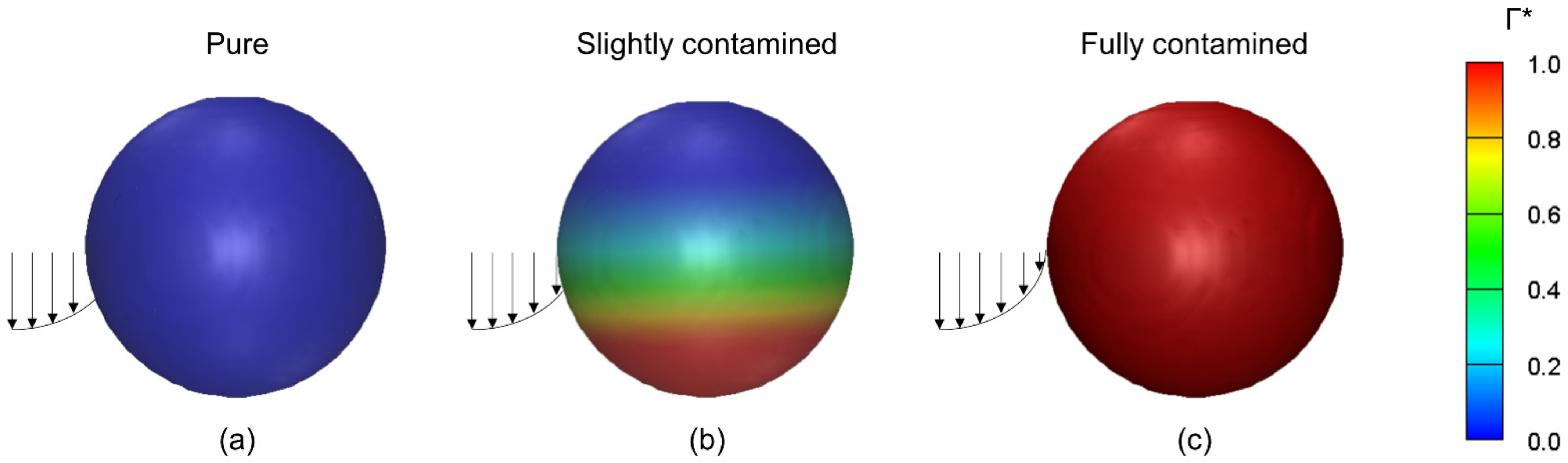
Influence of Contamination

The influence of contaminants and solid particles on the lift force has not been included to the discussion of the lift coefficient in the previous paragraph. However, it is known that their impact can be quite significant. In the above-discussed studies, the authors used purified water to minimize this effect. However, the pureness of this liquids varied and contamination sources, like moving parts in the rotating belt setup used by Tomiyama et al. [85], Dijkhuizen et al. [132], and Aoyama et al. [129], cause some level of uncertainty. As described in the subsequent section, this uncertainty complicates the comparability of the experimental studies, but may also explain some discrepancy of their results.

Ogasawara [135] experimentally observed that the tendency of small bubbles to cluster in the vicinity of the wall was reduced in case surfactants were added. Dijkhuizen et al. [132] used the rotating belt setup with tab water–glycerin mixtures to validate their numerical results. Here, they measured significantly lower lift coefficients for larger bubbles, but larger lift coefficients for smaller bubbles than predicted by the numerical results. In addition, they observed a shear flow dependency, which was not found numerically for pure liquids.

Influencing mechanisms of contaminations on the lift were also studied via numerical simulation. Fukuta et al. [105] found that the lift coefficient for a contaminated spherical bubble (Re = 100, Sr = 0.2) is significantly reduced and can become negative. To quantify the surfactant effects, they used the Langmuir number. As shown in Figure 17, it was found that in pure liquids, the total lift force (c_L) on small bubbles is mainly driven by pressure components (c_LP), while increasing surfactant levels decrease its impact until it disappears entirely, so that the small negative lift force is due to viscous stress (c_LV). Overall, the effect of surfactants was attributed to the Marangoni effect.

Hayashi and Tomiyama [136] expanded the range to larger bubbles, larger Langmuir numbers, and larger Hatta numbers (2 < Re < 70, 0.6 < Eo < 5, −6 < log₁₀(Mo) < −4, 0 < Sr < 1, 1.38 ≤ La ≤ 13.8, 0 < Ha < 41). Similarly, they found that the lift coefficient decreases with increasing Langmuir number. The main effect, however, depends on the Hatta number. In case of large Hatta numbers, which means that the absorption of contaminants is much faster than the bubble rising, the decrease of the lift coefficient is attributed to a decrease of the effective surface tension by:

$$\mathsf{\sigma }\left(\mathsf{\Gamma }\right){=\mathsf{\sigma }}_0\left[1+\frac{{\mathrm{R}}_{\mathrm{g}}{\mathrm{T}\mathsf{\Gamma }}_{\max }}{{\mathsf{\sigma }}_0}\ln (1-\frac{\mathsf{\Gamma }}{{\mathsf{\Gamma }}_{\max }})\right]$$

(67)

In that case, the Marangoni effect is negligible. The lift coefficient can be correlated with the modified Eötvös number, employing the effective surface tension. In case of smaller Hatta numbers, the Marangoni effect gains importance. They also found an effect of the shear rate, which they attributed to a slight flow induced inclination of the bubble for contaminated bubbles.

Rastello et al. [137] investigated the impact on hydrophobic tracer particles, that attach to the bubble, on the lift coefficient in a rotating flow in a cylinder (D = 100mm). They observed that clean bubbles have an unseparated wake while the wake of contaminated bubbles separates. In addition, the tracer induces a surface spinning, which results in a Magnus effect. In fact, fully contaminated bubbles rotated like solid particles. Thus, c_L increases due to this additional contribution of the Magnus effect, which itself depends on the shear rate. In contrast, Hessenkemper et al. [138] found no influence of tracer particles in a linear shear flow. Until further research has been conducted, one can only speculate about this discrepancy. Reasons can either be that the dimensionless shear rates investigated by Rastello were quite high (Sr > 0.2), the flow was rotating, the number of tracers attached to the bubble in the experiment by Hessenkemper et al. [138] were too small, or the tracer sizes were different and therefore the surface tension interaction of the particles with the bubbles was significantly different. Hessenkemper et al. [138] investigates the influence of inorganic surfactants. In contrast to organic surfactance, it was found that they increase the lift coefficient.

These studies reveal that the impact of surfactants and solid particles is far from being understood. It is likely that the different effects superimpose on each other, which complicates analysis further. In addition, the number of studies and their range is too limited to derive a comprehensive theory or a quantification of the effects to a wider range of physical conditions. Furthermore, there is currently no link between the described phenomena and measurable variables, so that a quantitative estimation of some of the mentioned influences in experimental measurements would be possible. On the other hand, the influence of contaminations might explain the good agreement with macroscale CFD models employing the Tomiyama correlation (Equation (61)) and measurements in water models. Because usually these models are filled with tab water and sometimes tracer particles are added, it might be that the extrapolation error is coincidentally mitigated by the contamination effect. This would also explain the discrepancy between early measurements of the lift coefficient in tap water [115,122] and more recent measurement in deionized water [133].

Unfortunately, measurements in liquid metals are lacking entirely. Because there is no comprehensive understanding of the lift force in pure liquids yet, the extrapolation of existing correlations to very low Morton number systems, like liquid metals, suffers from a very high degree of uncertainty. The study by Aoyama et al. [129] suggests that both the asymptotic limits of the lift coefficient for large and small bubbles, as well as the sign change and the slope around it, depend on the Morton number. In liquid metals, the Eötvös number is usually significantly larger than in the systems investigated. Therefore, existing correlations would predict negative lift coefficients even for small, approximately spherical bubbles. However, this contradicts its physical justification and is therefore very unlikely. For larger, presumably ellipsoidal bubbles, large negative values for c_L would be predicted, which is likely to lead to unphysical behavior and stability problems in numerical models. Therefore, in particular, the negative asymptotical limit of c_L for large bubble in liquid metals is of great interest. The discussion is further complicated by the large uncertainty of the prediction of the bubble’s deformation analyzed above, which is necessary for the calculation of the modified Eötvös number.

Another problem arises from the high surface tension of liquid metals. All experimental studies were made in systems with very low surface tension. The only evidence that the surface tension effect is entirely captured in the Morton number and modified Eötvös number was provided numerically by Bothe et al. [131], varying the surface tension from 0.1 to 0.8 N/m for pure liquids. However, in their study, systems with a significantly larger Morton number were investigated. Whether this relationship applies for higher surface tensions or if it can be reproduced experimentally cannot be predicted with the current knowledge. Even more difficult is the impact of surfactants and solid particles. It can be assumed that alloying elements and non-metallic inclusions affect the lift coefficient. However, it is likely that the strength of these effects is different from those observed in aqueous solutions because of the much higher surface tension. Finally, the lift coefficient may even change on the rising path of the bubbles due to the adherence of inclusions. Therefore, it is currently not possible to make reliable estimates about the lift force in metallurgical processes.

5.3. Virtual Mass Force

When a bubble rises through a liquid, some of the surrounding liquid is carried by the bubble. The virtual mass force is the force arising from the acceleration of the surrounding fluid. Since it virtually increases the mass of the bubble, it is called virtual mass force. It is given by [92]:

$${\mathrm{F}}_{\mathrm{VM}}={\mathrm{c}}_{\mathrm{VM}}{\mathsf{\rho }}_{\mathrm{l}}{\mathrm{V}}_{\mathrm{b}}\left(\frac{{\mathrm{du}}_{\mathrm{l}}}{\mathrm{dt}}-\frac{{\mathrm{du}}_{\mathrm{b}}}{\mathrm{dt}}\right)$$

(68)

The virtual mass force limits the bubble acceleration. Thus, it is important to stabilize numerical calculations [139]. Like the drag force and the lift force, the virtual mass force is proportional to a coefficient c_VM, by which all influences on the force are represented. If c_VM is too small, the bubble acceleration may become too large, which can cause numerical instability depending on the solution process and settings. If c_VM is too large, the acceleration phase becomes unphysically long and smaller oscillations in the bubble’s rising path may be suppressed. For a spherical bubble in stagnant liquids, an analytical value of c_VM = 0.5 was derived [140]. This value is also used in almost all numerical studies. There are only a small number of quantitative studies on the exact value of c_VM in real flow conditions. These suggest that the value of c_VM also depends on the void fraction [141,142] and the bubble deformation ([143] found in [144]). However, if acceleration effects are not significant in the flow, then the virtual mass force is not important for the flow either. This applies, for example, to bubble reactors [142]. Therefore, the exact knowledge of c_VM plays a minor role in this type of flow.

6. Discussion

Despite numerous studies and many years of research, the dynamics of gas bubbles are not yet fully understood. This applies in particular to liquid metals, where even experiments to verify existing correlations are difficult, if possible at all, and place the highest demands on measurement techniques. In this review, the transferability of correlations from more accessible systems to liquid metals was analyzed. In this concluding discussion, the results are briefly summarized and approaches to resolve existing uncertainties are proposed.

The same formation regimes as in water models had been observed on single nozzles in liquid metals. However, the mechanisms differ with respect to wettability of the nozzle. For higher, more industrially relevant flow rates, this effect seems to decrease in relevance. Instead, the bubble size distribution is mainly determined by coalescence and especially breakup. The bubble formation mechanism is different at purging plugs than at single nozzles and presumably other bubble size distributions are generated. However, coalescence, rather than breakup, has a decisive role here. Extrapolating observations made in aqueous systems, it can be assumed that the bubble column in most processes is in the heterogeneous regime and the bubble size distribution follows a log-normal distribution. However, a verification of this assumption in liquid metals is difficult because relatively large experimental setups are needed, which exceed the limits of most available measurement techniques today. The only exception so far are resistivity probes, which are intrusive and consequently introduce a bias into the measurements. Therefore, the real bubble size distribution in industrial plants can only be predicted with considerable uncertainty, as the example of a ladle shows. For specific applications, such as the ladle, resistivity probe measurements in the real process can provide a reasonable estimate of the bubble size distribution. However, these measurements will be associated with difficulties such as the measurement bias and the short lifetime of the sensors at high temperatures [21]. More importantly, the bubble size distribution depends on local flow conditions and the type of gas injection, so that results of such measurements can hardly be generalized. Therefore, to predict the bubble size distribution in different processes, it is essential to develop a more detailed understanding of the coalescence and breakup mechanisms. This will be a major experimental challenge even in aqueous systems, since the instantaneous flow field and the behavior of bubbles have to be measured simultaneously in three dimensions. In liquid metals, this is currently not possible, although there is a first approach to simultaneously measure the flow and bubbles in two dimensions [29]. Studies in liquid metals like those by Keplinger et al. [22,75] can be used to critically discuss the scalability of mechanisms investigated in aqueous models, even though the physical restrictions of imaging techniques in liquid metals allow for a significantly lower degree of detail. Due to the difficulty of the experiments, DNS could be a useful alternative to develop fundamental knowledge of coalescence and breakup mechanisms. Nevertheless, this requires further development of phase boundary modeling, and these calculations will be highly computationally expensive. Once the coalescence and breakup mechanisms are sufficiently understood, these fundamental insights can be transferred to the reactor scale using PBMs. Since the first experiments in liquid metals suggest that turbulence effects are inherently important, at least an LES approach should be chosen. For a precise validation of such PBMs, however, exact experimental benchmark cases are necessary. For these benchmark cases it is important that all boundary conditions are reported in detail and the measurement uncertainty can be quantified [14].

A comparison of different bubble deformation models and experimental measurements in liquid metals revealed that these models, derived for aqueous systems, significantly overestimate the deformation. The best agreement was found with the model of Wellek et al. [81] for contaminated systems. This result can be interpreted in different ways. First, the less pronounced deformation could indicate that the examined liquid metal systems were contaminated, since, for example, they were partially oxidized. Another explanation is that the deformation has a dependence on the fluid properties that is not yet fully understood. Indeed, there are few measurements on systems with Morton numbers smaller than water, which approximately correspond to the values of liquid metals. A final assessment of which explanation applies cannot be made due to the small number of experimental studies. Experiments with high-purity metals in an inert gas atmosphere could provide new insights here.

Besides the influence of contaminants, other factors can introduce an uncertainty to the measurement of bubble deformation. These can partly explain the distinct differences of existing models and should be taken into account in the design and evaluation of future measurements of bubble deformation in liquid metals. Especially in shallow experimental setups, there may be an influence of the injector. When the bubble is released from the injector, a strong deformation occurs, which is subsequently damped. If the measuring point is too close to the injector, the results may be biased. This can be a particular problem for measurements in liquid metals, where the measurement volumes are often quite small. Therefore, a sufficient filling height must be ensured and an influence of the injector should be examined, for example by using different injectors. Other problems arise from the physical restrictions of imaging techniques such as X-ray or neutron radiography measurements. An influence of the walls on the deformation may arise due to the small thickness of the measurement volume. Furthermore, this limits the measurements to relatively small bubbles, so extrapolation of deformation models to larger bubbles will remain a problem. Finally, it should be considered that a measurement uncertainty arises from the reconstruction of the three-dimensional bubble shape by a single two-dimensional projection [13]. On the other hand, the alternative usage of multi-needle resistivity probes has the drawback of being intrusive.

Even though the number of experimental measurements is too small for a conclusive assessment, the drag force seems to be predictable employing existing correlations. The frequently used correlation according to Tomiyama et al. [95] generally provides reasonable accordance with measurements in liquid metals. For smaller bubbles, there is some uncertainty due to the influence of contaminants. [19] Additionally, the influence of surrounding bubbles in a bubble swarm on the drag coefficient in liquid metals cannot be quantified yet. Nevertheless, employing existing measurement methods, it should be possible to further refine the knowledge of the drag force in liquid metals. For this purpose, bubble swarms as well as single bubbles of different size should be examined. One challenge is the generation of single large bubbles, which is difficult to control by nozzles. For this purpose, a rotating cup as proposed by Davenport [19] might be used.

For the lift force there is no comprehensive understanding even for aqueous systems. For liquid metals, experimental data are lacking entirely. From a numerical point of view, it seems reasonable to define an asymptotic limit for negative values similar to Frank et al. [96], to prevent numerical instability. However, these values are currently highly uncertain for liquid metal systems and there is probably a dependency of the lift force on the Morton number, which is not yet quantifiable. Experimentally, it will be very difficult to determine the lift coefficient for liquid metals since an exactly defined shear flow must be generated, which is difficult to control in liquid metal systems. A possible solution might be a bubble column induced shear flow proposed by Ziegenhein et al. [133]. This shear flow could be quantified by NeuPIV [29], simultaneously measuring the rising path of a single bubble. On the other hand, given that the experimental setup has to the thin to employ neutron radiography, the influence of the walls might prevent a defined shear flow.

When considering metallurgical reactors, the virtual mass force seems mostly important for numerical stability and has little effect on the flow. The currently most frequently used value of 0.5 for the virtual mass coefficient seems to be sufficiently accurate in almost all cases.

A fundamental problem in the scaling of all described phenomena is that the dynamics of bubbles are strongly influenced by contaminants. However, with the current state of knowledge, it is not possible to conclusively assess whether contaminants are relevant in industrial processes, too. It can even be assumed that the influence changes during the process. It can be speculated whether contaminants have an influence on the conductivity of the melt and can therefore be quantified. However, this remains speculative at the present state of knowledge. Moreover, it is unknown whether contaminants have the same effect in liquid metals as in aqueous systems. Fundamental research in the field of molecular dynamics could provide new insights into this topic.

In summary, the behavior of gas bubbles in liquid metals is still far from being fully understood. This leads to a considerable uncertainty of numerical models of metallurgical reactors involving bubble flows. However, some direct measurement techniques have been developed in recent years that allow a more detailed analysis of different phenomena. Using these methods, further measurements should be carried out to reduce the lack of experimental data in liquid metals. With more experimental data, especially for value ranges and phenomena that have not yet been sufficiently analyzed, the discussion of the scalability of existing models can be significantly improved. This could help to reduce many of the remaining knowledge gaps in the future.

References

1. Deckwer, W.-D.; Field, R.W. Bubble Column Reactors; Wiley: New York, NY, USA, 1992; Volume 200. [Google Scholar]
2. Prosperetti, A. Bubbles. Phys. Fluids 2004, 16, 1852–1865. [Google Scholar] [CrossRef]
3. Besagni, G.; Inzoli, F.; Ziegenhein, T. Two-phase bubble columns: A comprehensive review. ChemEngineering 2018, 2, 13. [Google Scholar] [CrossRef] [Green Version]
4. Veldhuis, C.; Biesheuvel, A.; Van Wijngaarden, L. Shape oscillations on bubbles rising in clean and in tap water. Phys. Fluids 2008, 20, 040705. [Google Scholar] [CrossRef]
5. Sanada, T.; Sugihara, K.; Shirota, M.; Watanabe, M. Motion and drag of a single bubble in super-purified water. Fluid Dynam. Res. 2008, 40, 534. [Google Scholar] [CrossRef]
6. Fu, Y.; Liu, Y. Development of a robust image processing technique for bubbly flow measurement in a narrow rectangular channel. Int. J. Multiph. Flow 2016, 84, 217–228. [Google Scholar] [CrossRef]
7. Bröder, D.; Sommerfeld, M. Planar shadow image velocimetry for the analysis of the hydrodynamics in bubbly flows. Meas. Sci. Technol. 2007, 18, 2513. [Google Scholar] [CrossRef]
8. Ferreira, A.; Pereira, G.; Teixeira, J.; Rocha, F. Statistical tool combined with image analysis to characterize hydrodynamics and mass transfer in a bubble column. Chem. Eng. J. 2012, 180, 216–228. [Google Scholar] [CrossRef] [Green Version]
9. Karn, A.; Ellis, C.; Arndt, R.; Hong, J. An integrative image measurement technique for dense bubbly flows with a wide size distribution. Chem. Eng. Sci. 2015, 122, 240–249. [Google Scholar] [CrossRef] [Green Version]
10. Lau, Y.; Sujatha, K.T.; Gaeini, M.; Deen, N.; Kuipers, J. Experimental study of the bubble size distribution in a pseudo-2D bubble column. Chem. Eng. Sci. 2013, 98, 203–211. [Google Scholar] [CrossRef]
11. Poletaev, I.; Pervunin, K.; Tokarev, M. Artificial neural network for bubbles pattern recognition on the images. J. Phys. Conf. Ser. 2016, 754, 072002. [Google Scholar] [CrossRef] [Green Version]
12. Haas, T.; Schubert, C.; Eickhoff, M.; Pfeifer, H. BubCNN: Bubble detection using Faster RCNN and shape regression network. Chem. Eng. Sci. 2020. [Google Scholar] [CrossRef]
13. Fu, Y.; Liu, Y. 3D bubble reconstruction using multiple cameras and space carving method. Meas. Sci. Technol. 2018, 29, 075206. [Google Scholar] [CrossRef]
14. Haas, T.; Suarez, A.L.; Eickhoff, M.; Pfeifer, H. Toward a Strong-Sense Validation Benchmark Database for Numerical Ladle Flow Models. Metal. Mater. Trans. B 2021, 52, 199–222. [Google Scholar] [CrossRef]
15. Sano, M.; Mori, K. Bubble formation from single nozzles in liquid metals. Trans. Jpn. Instit. Metals 1976, 17, 344–352. [Google Scholar] [CrossRef] [Green Version]
16. Tsuchiya, K.; Aida, M.; Fujii, Y.; Okamoto, M. Bubble formation from a single nozzle in moderator liquids and liquid metal for tritium breeding. J. Nucl. Mater. 1993, 207, 123–129. [Google Scholar] [CrossRef]
17. Andreini, R.; Foster, J.; Callen, R. Characterization of gas bubbles injected into molten metals under laminar flow conditions. Metal. Trans. B 1977, 8, 625–631. [Google Scholar] [CrossRef]
18. Irons, G.; Guthrie, R. Bubble formation at nozzles in pig iron. Metal. Trans. B 1978, 9, 101–110. [Google Scholar] [CrossRef]
19. Davenport, W.G. Bubbles in Liquids Including Liquid Metals; The Royal School of Mines: London, UK, 1964. [Google Scholar]
20. Mori, K.; Ozawa, Y.; Sano, M. Characterization of gas jet behavior at a submerged orifice in liquid metal. Trans. Iron Steel Inst. Jpn. 1982, 22, 377–384. [Google Scholar] [CrossRef]
21. Iguchi, M.; Kawabata, H.; Nakajima, K.; Morita, Z.-I. Measurement of bubble characteristics in a molten iron bath at 1600 °C using an electroresistivity probe. Metal. Mater. Trans. B 1995, 26, 67–74. [Google Scholar] [CrossRef]
22. Keplinger, O.; Shevchenko, N.; Eckert, S. Visualization of bubble coalescence in bubble chains rising in a liquid metal. Int. J. Multiph. Flow 2018, 105, 159–169. [Google Scholar] [CrossRef]
23. Iguchi, M.; Nakatani, T.; Tokunaga, H. The shape of bubbles rising near the nozzle exit in molten metal baths. Metal. Mater. Trans. B 1997, 28, 417–423. [Google Scholar] [CrossRef]
24. Iguchi, M.; Nakatani, T.; Kawabata, H. Development of a multineedle electroresistivity probe for measuring bubble characteristics in molten metal baths. Metal. Mater. Trans. B 1997, 28, 409–416. [Google Scholar] [CrossRef]
25. Davis, K.G.; Irons, G.A.; Guthrie, R.I.L. X-ray cinematographic observations of gas injection into liquid metals. Metal. Mater. Trans. B 1978, 9, 721–722. [Google Scholar] [CrossRef]
26. Iguchi, M.; Chihara, T.; Takanashi, N.; Ogawa, Y.; Tokumitsu, N.; Morita, Z.-I. X-ray fluoroscopic observation of bubble characteristics in a molten iron bath. ISIJ Int. 1995, 35, 1354–1361. [Google Scholar] [CrossRef]
27. Keplinger, O.; Shevchenko, N.; Eckert, S. Validation of X-ray radiography for characterization of gas bubbles in liquid metals. IOP Conf. Ser. Mater. Sci. Eng. 2017, 228, 012009. [Google Scholar] [CrossRef] [Green Version]
28. Mishima, K.; Hibiki, T.; Saito, Y.; Nishihara, H.; Tobita, Y.; Konishi, K.; Matsubayashi, M. Visualization and measurement of gas–liquid metal two-phase flow with large density difference using thermal neutrons as microscopic probes. Nucl. Instrum. Methods Phys. Res. Sect. A Accel. Spectromet. Detect. Assoc. Equip. 1999, 424, 229–234. [Google Scholar] [CrossRef]
29. Sarma, M.; Ščepanskis, M.; Jakovičs, A.; Thomsen, K.; Nikoluškins, R.; Vontobel, P.; Beinerts, T.; Bojarevičs, A.; Platacis, E. Neutron radiography visualization of solid particles in stirring liquid metal. Phys. Proc. 2015, 69, 457–463. [Google Scholar] [CrossRef] [Green Version]
30. Baake, E.; Fehling, T.; Musaeva, D.; Steinberg, T. Neutron radiography for visualization of liquid metal processes: Bubbly flow for CO2 free production of Hydrogen and solidification processes in EM field. IOP Conf. Ser. Mater. Sci. Eng. 2017, 228, 12026. [Google Scholar] [CrossRef]
31. Richter, T.; Keplinger, O.; Strumpf, E.; Wondrak, T.; Eckert, K.; Eckert, S.; Odenbach, S. Measurements of the Diameter of Rising Gas Bubbles by Means of the Ultrasound Transit Time Technique. Magnetohydrodynamics (0024-998X) 2017, 53, 383–392. [Google Scholar] [CrossRef]
32. Wang, Z.; Wang, S.; Meng, X.; Ni, M. UDV measurements of single bubble rising in a liquid metal Galinstan with a transverse magnetic field. Int. J. Multiph. Flow 2017, 94, 201–208. [Google Scholar] [CrossRef]
33. Gundrum, T.; Büttner, P.; Dekdouk, B.; Peyton, A.; Wondrak, T.; Galindo, V.; Eckert, S. Contactless inductive bubble detection in a liquid metal flow. Sensors 2016, 16, 63. [Google Scholar] [CrossRef] [Green Version]
34. Karcher, C.; Lyu, Z.; Boeck, T.; Tran, N.; Lüdtke, U. Experimental and numerical investigation on particle-induced liquid metal flow using Lorentz force velocimetry. IOP Conf. Ser. Mater. Sci. Eng. 2018, 424, 1. [Google Scholar] [CrossRef]
35. Zhang, L.; Taniguchi, S. Fundamentals of inclusion removal from liquid steel by bubble flotation. Int. Mater. Rev. 2000, 45, 59–82. [Google Scholar] [CrossRef]
36. Stapurewicz, T.; Themelis, N.J. Mixing and mass transfer phenomena in bottom-injected gas–liquid reactors. Can. Metal. Quart. 1987, 26, 123–128. [Google Scholar] [CrossRef]
37. Owusu, K.B.; Haas, T.; Gajjar, P.; Eickhoff, M.; Kowitwarangkul, P.; Pfeifer, H. Interaction of Injector Design, Bubble Size, Flow Structure, and Turbulence in Ladle Metallurgy. Steel Res. Int. 2019, 90, 1800346. [Google Scholar] [CrossRef]
38. Haas, T.; Schubert, C.; Eickhoff, M.; Pfeifer, H. Numerical modeling of the ladle flow by a LES-based Eulerian-Lagrange approach: A systematic survey. Metal. Mater. Trans. B 2021, 52, 903–921. [Google Scholar] [CrossRef]
39. Kraume, M.; Zehner, P. Modellierung der Fluiddynamik in Blasensäulen. Chemieingenieurtechnik 1989, 61, 332–333. [Google Scholar] [CrossRef]
40. Kulkarni, A.A.; Joshi, J.B. Bubble formation and bubble rise velocity in gas− liquid systems: A review. Ind. Eng. Chem. Res. 2005, 44, 5873–5931. [Google Scholar] [CrossRef]
41. Leibson, I.; Holcomb, E.G.; Cacoso, A.G.; Jacmic, J.J. Rate of flow and mechanics of bubble formation from single submerged orifices. I. Rate of flow studies. AIChE J. 1956, 2, 296–300. [Google Scholar] [CrossRef]
42. Sano, M.; Mori, K. Size of bubbles in energetic gas injection into liquid metal. Trans. Iron Steel Inst. Jpn. 1980, 20, 675–681. [Google Scholar] [CrossRef] [Green Version]
43. Tate, T. On the magnitude of a drop of liquid formed under different circumstances. Lond. Edinb. Dublin Philos. Magaz. J. Sci. 1864, 27, 176–180. [Google Scholar] [CrossRef]
44. Davidson, L.; Amick, E.H., Jr. Formation of gas bubbles at horizontal orifices. AIChE J. 1956, 2, 337–342. [Google Scholar] [CrossRef]
45. Mersmann, A. Druckverlust und Schaumhöhen von gasdurchströmten Flüssigkeitsschichten auf Siebböden. VDI ForschHft B 1962, 28, 144. [Google Scholar]
46. Mori, K.; Sano, M.; Sato, T. Size of bubbles formed at single nozzle immersed in molten iron. Trans. Iron Steel Inst. Jpn. 1979, 19, 553–558. [Google Scholar] [CrossRef]
47. Xie, Y.; Orsten, S.; Oeters, F. Behaviour of bubbles at gas blowing into liquid Wood’s metal. ISIJ Int. 1992, 32, 66–75. [Google Scholar] [CrossRef] [Green Version]
48. Gnyloskurenko, S.V.; Nakamura, T. Wettability effect on bubble formation at nozzles in liquid aluminum. Mater. Trans. 2003, 44, 2298–2302. [Google Scholar] [CrossRef] [Green Version]
49. Zhang, L.; Taniguchi, S.; Matsumoto, K. Water model study on inclusion removal from liquid steel by bubble flotation under turbulent conditions. Ironmak. Steelmak. 2002, 29, 326–336. [Google Scholar] [CrossRef]
50. Iguchi, M.; Tokunaga, H.; Tatemichi, H. Bubble and liquid flow characteristics in a wood’s metal bath stirred by bottom helium gas injection. Metal. Mater. Trans. B 1997, 28, 1053–1061. [Google Scholar] [CrossRef]
51. Castillejos, A.; Brimacombe, J. Physical characteristics of gas jets injected vertically upward into liquid metal. Metal. Trans. B 1989, 20, 595–601. [Google Scholar] [CrossRef]
52. Houghton, G.; McLean, A.; Ritchie, P. Mechanism of formation of gas bubble-beds. Chem. Eng. Sci. 1957, 7, 40–50. [Google Scholar] [CrossRef]
53. Loimer, T.; Machu, G.; Schaflinger, U. Inviscid bubble formation on porous plates and sieve plates. Chem. Eng. Sci. 2004, 59, 809–818. [Google Scholar] [CrossRef]
54. Mirsandi, H.; Baltussen, M.; Peters, E.; van Odyck, D.; van Oord, J.; van der Plas, D.; Kuipers, J. Numerical simulations of bubble formation in liquid metal. Int. J. Multiph. Flow 2020, 131, 103363. [Google Scholar] [CrossRef]
55. Wang, Z.; Mukai, K.; Izu, D. Influence of wettability on the behavior of argon bubbles and fluid flow inside the nozzle and mold. ISIJ Int. 1999, 39, 154–163. [Google Scholar] [CrossRef]
56. Koide, K.; Kato, S.; Tanaka, Y.; Kubota, H. Bubbles generated from porous plate. J. Chem. Eng. Jpn. 1968, 1, 51–56. [Google Scholar] [CrossRef] [Green Version]
57. Baxter, R.; Wraith, A. Transitions in the bubble formation mode of a submerged porous disc. Chem. Eng. Sci. 1970, 25, 1244–1247. [Google Scholar] [CrossRef]
58. Anagbo, P.; Brimacombe, J. Plume characteristics and liquid circulation in gas injection through a porous plug. Metal. Trans. B 1990, 21, 637–648. [Google Scholar] [CrossRef]
59. Goyal, P.; Themelis, N.; Zanchuk, W.A. Gaseous refining of anode copper. JOM 1982, 34, 22–28. [Google Scholar] [CrossRef]
60. Iguchi, M.; Kaji, M.; Morita, Z.-I. Effects of pore diameter, bath surface pressure, and nozzle diameter on the bubble formation from a porous nozzle. Metal. Mater. Trans. B 1998, 29, 1209–1218. [Google Scholar] [CrossRef]
61. Kazakis, N.; Papadopoulos, I.; Mouza, A. Bubble columns with fine pore sparger operating in the pseudo-homogeneous regime: Gas hold up prediction and a criterion for the transition to the heterogeneous regime. Chem. Eng. Sci. 2007, 62, 3092–3103. [Google Scholar] [CrossRef]
62. Mohagheghian, S.; Ghajar, A.J.; Elbing, B. Effect of operation regime on bubble size and void fraction in a bubble column with porous sparger. Authorea Prepr. 2020. [Google Scholar] [CrossRef]
63. Lucas, D.; Ziegenhein, T. Influence of the bubble size distribution on the bubble column flow regime. Int. J. Multiph. Flow 2019, 120, 103092. [Google Scholar] [CrossRef]
64. Koide, K.; Hayashi, T.; Noro, M.; Takemura, Y.; Kawamata, N.; Kubota, H. Bubbles generated from porous plate in pure liquid and in aqueous solutions of inorganic electrolytes. J. Chem. Eng. Jpn. 1972, 5, 236–242. [Google Scholar] [CrossRef] [Green Version]
65. Miyahara, T.; Tanaka, A. Size of bubbles generated from porous plates. J. Chem. Eng. Jpn. 1997, 30, 353–355. [Google Scholar] [CrossRef] [Green Version]
66. Li, R.-Q.; Harris, R. Bubble formation from a very narrow slot. Can. Metal. Quart. 1993, 32, 31–37. [Google Scholar] [CrossRef]
67. Li, R.-Q.; Wraith, A.; Harris, R. Gas dispersion phenomena at a narrow slot submerged in a liquid. Chem. Eng. Sci. 1994, 49, 531–540. [Google Scholar] [CrossRef]
68. Wraith, A.; Li, R.-Q.; Harris, R. Gas bubble volume at a narrow slot nozzle in a liquid. Chem. Eng. Sci. 1995, 50, 1057–1058. [Google Scholar] [CrossRef]
69. Harris, R.; Ng, K.; Wraith, A. Spargers for controlled bubble size by means of the multiple slot disperser (MSD). Chem. Eng. Sci. 2005, 60, 3111–3115. [Google Scholar] [CrossRef]
70. Okumura, K.; Harrist, R.; Sanot, M. Bubble formation from nonwetted slot nozzles. Can. Metal. Quart. 1998, 37, 49–56. [Google Scholar] [CrossRef]
71. Okumura, K.; Komarov, S.V.; Sano, M. Gas injection from slot nozzles with various shapes in water. ISIJ Int. 2000, 40, 544–548. [Google Scholar] [CrossRef]
72. Trummer, B.; Fellner, W.; Viertauer, A.; Kneis, L.; Hackl, G. A Water Modelling Comparison of Hybrid Plug, Slot Plug and Porous Plug Designs. RHI Worldwide 2016, 1, 35. [Google Scholar]
73. Polli, M.; Di Stanislao, M.; Bagatin, R.; Bakr, E.A.; Masi, M. Bubble size distribution in the sparger region of bubble columns. Chem. Eng. Sci. 2002, 57, 197–205. [Google Scholar] [CrossRef]
74. Liao, Y.; Lucas, D. A literature review of theoretical models for drop and bubble breakup in turbulent dispersions. Chem. Eng. Sci. 2009, 64, 3389–3406. [Google Scholar] [CrossRef]
75. Keplinger, O.; Shevchenko, N.; Eckert, S. Experimental investigation of bubble breakup in bubble chains rising in a liquid metal. Int. J. Multiph. Flow 2019, 116, 39–50. [Google Scholar] [CrossRef]
76. Liao, Y.; Lucas, D. A literature review on mechanisms and models for the coalescence process of fluid particles. Chem. Eng. Sci. 2010, 65, 2851–2864. [Google Scholar] [CrossRef]
77. Sahai, Y.; Guthrie, R. Hydrodynamics of gas stirred melts: Part I. Gas/liquid coupling. Metal. Trans. B 1982, 13, 193–202. [Google Scholar] [CrossRef]
78. Moore, D. The velocity of rise of distorted gas bubbles in a liquid of small viscosity. J. Fluid Mech. 1965, 23, 749–766. [Google Scholar] [CrossRef]
79. Bozzano, G.; Dente, M. Shape and terminal velocity of single bubble motion: A novel approach. Comp. Chem. Eng. 2001, 25, 571–576. [Google Scholar] [CrossRef]
80. Liang-Shih, F.; Tsuchiya, K. Bubble Wake Dynamics in Liquids and Liquid-Solid Suspensions; Butterworth-Heinemann: Oxford, UK, 2013. [Google Scholar]
81. Wellek, R.; Agrawal, A.; Skelland, A. Shape of liquid drops moving in liquid media. AIChE J. 1966, 12, 854–862. [Google Scholar] [CrossRef]
82. Clift, R.; Grace, J.R.; Weber, M.E. Bubbles, Drops, and Particles; Courier Corporation: Chelmsford, MA, USA, 2005. [Google Scholar]
83. Aoyama, S.; Hayashi, K.; Hosokawa, S.; Tomiyama, A. Shapes of single bubbles in infinite stagnant liquids contaminated with surfactant. Exp. Therm. Fluid Sci. 2018, 96, 460–469. [Google Scholar] [CrossRef]
84. Besagni, G.; Deen, N.G. Aspect ratio of bubbles in different liquid media: A novel correlation. Chem. Eng. Sci. 2020, 215, 115383. [Google Scholar] [CrossRef]
85. Tomiyama, A.; Tamai, H.; Zun, I.; Hosokawa, S. Transverse migration of single bubbles in simple shear flows. Chem. Eng. Sci. 2002, 57, 1849–1858. [Google Scholar] [CrossRef]
86. Vakhrushev, I.; Efremov, G. Interpolation formula for computing the velocities of single gas bubbles in liquids. Chem. Technol. Fuels Oils 1970, 6, 376–379. [Google Scholar] [CrossRef]
87. Aoyama, S.; Hayashi, K.; Hosokawa, S.; Tomiyama, A. Shapes of ellipsoidal bubbles in infinite stagnant liquids. Int. J. Multiph. Flow 2016, 79, 23–30. [Google Scholar] [CrossRef]
88. Ziegenhein, T.; Lucas, D. Observations on bubble shapes in bubble columns under different flow conditions. Exp. Therm. Fluid Sci. 2017, 85, 248–256. [Google Scholar] [CrossRef]
89. Dijkhuizen, W.; Roghair, I.; Annaland, M.V.S.; Kuipers, J. DNS of gas bubbles behaviour using an improved 3D front tracking model—Drag force on isolated bubbles and comparison with experiments. Chem. Eng. Sci. 2010, 65, 1415–1426. [Google Scholar] [CrossRef]
90. Xu, Y.; Ersson, M.; Jönsson, P. Numerical simulation of single argon bubble rising in molten metal under a laminar flow. Steel Res. Int. 2015, 86, 1289–1297. [Google Scholar] [CrossRef]
91. Wang, G.; Zhou, H.; Tian, Q.; Ai, X.; Zhang, L. The Motion of Single Bubble and Interactions between Two Bubbles in Liquid Steel. ISIJ Int. 2017. [Google Scholar] [CrossRef] [Green Version]
92. Magnaudet, J.; Eames, I. The motion of high-Reynolds-number bubbles in inhomogeneous flows. Annu. Rev. Fluid Mech. 2000, 32, 659–708. [Google Scholar] [CrossRef]
93. Mei, R.; Klausner, J.F. Unsteady force on a spherical bubble at finite Reynolds number with small fluctuations in the free-stream velocity. Phys. Fluids A Fluid Dynam. 1992, 4, 63–70. [Google Scholar] [CrossRef]
94. Pang, M.J.; Wei, J.J. Analysis of drag and lift coefficient expressions of bubbly flow system for low to medium Reynolds number. Nucl. Eng. Design 2011, 241, 2204–2213. [Google Scholar] [CrossRef]
95. Tomiyama, A.; Kataoka, I.; Zun, I.; Sakuguchi, T. Drag Coefficients of Single Bubbles under Normal and Micro Gravity Conditions. JSME Int. J. Ser. B Fluids Therm. Eng. 1998, 41, 472–479. [Google Scholar] [CrossRef]
96. Frank, T.; Shi, J.; Burns, A. Validation of Eulerian multiphase flow models for nuclear safety applications. In Proceedings of the 3rd International Symposium on Two-Phase Flow Modelling and Experimentation, Pisa, Italy, 22–24 September 2014. [Google Scholar]
97. Peebles, F.; Garber, H. Studies on the Motion of Gas Bubbles in Liquids. Chem. Eng. Progress 1953, 49, 88–97. [Google Scholar]
98. Mori, Y.; Hijikata, K.; Kuriyama, I. Experimental study of bubble motion in mercury with and without a magnetic field. J. Heat Transfer 1977, 99, 404–410. [Google Scholar] [CrossRef]
99. Zhang, C.; Eckert, S.; Gerbeth, G. Experimental study of single bubble motion in a liquid metal column exposed to a DC magnetic field. Int. J. Multiph. Flow 2005, 31, 824–842. [Google Scholar] [CrossRef]
100. Takagi, S.; Matsumoto, Y. Surfactant effects on bubble motion and bubbly flows. Annu. Rev. Fluid Mech. 2011, 43, 615–636. [Google Scholar] [CrossRef]
101. Tasoglu, S.; Demirci, U.; Muradoglu, M. The effect of soluble surfactant on the transient motion of a buoyancy-driven bubble. Phys. Fluids 2008, 20, 040805. [Google Scholar] [CrossRef] [Green Version]
102. Cuenot, B.; Magnaudet, J.; Spennato, B. The effects of slightly soluble surfactants on the flow around a spherical bubble. J. Fluid Mech. 1997, 339, 25–53. [Google Scholar] [CrossRef]
103. Zhang, Y.; Finch, J. A note on single bubble motion in surfactant solutions. J. Fluid Mech. 2001, 429, 63. [Google Scholar] [CrossRef]
104. Takagi, S.; Ogasawara, T.; Matsumoto, Y. The effects of surfactant on the multiscale structure of bubbly flows. Philos. Trans. R. Soc. A Math. Phys. Eng. Sci. 2008, 366, 2117–2129. [Google Scholar] [CrossRef]
105. Fukuta, M.; Takagi, S.; Matsumoto, Y. Numerical study on the shear-induced lift force acting on a spherical bubble in aqueous surfactant solutions. Phys. Fluids 2008, 20, 040704. [Google Scholar] [CrossRef]
106. Simonnet, M.; Gentric, C.; Olmos, E.; Midoux, N. Experimental determination of the drag coefficient in a swarm of bubbles. Chem. Eng. Sci. 2007, 62, 858–866. [Google Scholar] [CrossRef]
107. Richardson, J.; Zaki, W. The sedimentation of a suspension of uniform spheres under conditions of viscous flow. Chem. Eng. Sci. 1954, 3, 65–73. [Google Scholar] [CrossRef]
108. Lockett, M.J.; Kirkpatrick, R.D. Ideal bubbly flow and actual flow in bubble columns. Trans. Inst. Chem. Eng. 1975, 53, 267–273. [Google Scholar]
109. Garnier, C.; Lance, M.; Marié, J. Measurement of local flow characteristics in buoyancy-driven bubbly flow at high void fraction. Exp. Therm. Fluid Sci. 2002, 26, 811–815. [Google Scholar] [CrossRef]
110. Guet, S.; Ooms, G.; Oliemans, R.; Mudde, R. Bubble size effect on low liquid input drift–flux parameters. Chem. Eng. Sci. 2004, 59, 3315–3329. [Google Scholar] [CrossRef]
111. Roghair, I.; Lau, Y.; Deen, N.; Slagter, H.; Baltussen, M.; Annaland, M.V.S.; Kuipers, J. On the drag force of bubbles in bubble swarms at intermediate and high Reynolds numbers. Chem. Eng. Sci. 2011, 66, 3204–3211. [Google Scholar] [CrossRef]
112. Grienberger, J.; Hofmann, H. Investigations and modelling of bubble columns. Chem. Eng. Sci. 1992, 47, 2215–2220. [Google Scholar] [CrossRef]
113. Simonnet, M.; Gentric, C.; Olmos, E.; Midoux, N. CFD simulation of the flow field in a bubble column reactor: Importance of the drag force formulation to describe regime transitions. Chem. Eng. Proces. Process Intensif. 2008, 47, 1726–1737. [Google Scholar] [CrossRef]
114. Lau, Y.; Roghair, I.; Deen, N.; van Sint Annaland, M.; Kuipers, J. Numerical investigation of the drag closure for bubbles in bubble swarms. Chem. Eng. Sci. 2011, 66, 3309–3316. [Google Scholar] [CrossRef]
115. Zun, I. The transverse migration of bubbles influenced by walls in vertical bubbly flow. Int. J. Multiph. Flow 1980, 6, 583–588. [Google Scholar] [CrossRef]
116. Saffman, P. The lift on a small sphere in a slow shear flow. J. Fluid Mech. 1965, 22, 385–400. [Google Scholar] [CrossRef] [Green Version]
117. McLaughlin, J.B. Inertial migration of a small sphere in linear shear flows. J. Fluid Mech. 1991, 224, 261–274. [Google Scholar] [CrossRef]
118. Legendre, D.; Magnaudet, J. A note on the lift force on a spherical bubble or drop in a low-Reynolds-number shear flow. Phys. Fluids 1997, 9, 3572–3574. [Google Scholar] [CrossRef] [Green Version]
119. Mei, R.; Klausner, J. Shear lift force on spherical bubbles. Int. J. Heat Fluid Flow 1994, 15, 62–65. [Google Scholar] [CrossRef]
120. Auton, T. The lift force on a spherical body in a rotational flow. J. Fluid Mech. 1987, 183, 199–218. [Google Scholar] [CrossRef]
121. Legendre, D.; Magnaudet, J. The lift force on a spherical bubble in a viscous linear shear flow. J. Fluid Mech. 1998, 368, 81–126. [Google Scholar] [CrossRef]
122. Lance, M.; De Bertodano, M.L. Phase distribution phenomena and wall effects in bubbly two-phase flows. Multiph. Sci. Technol. 1994, 8. [Google Scholar] [CrossRef]
123. Liu, T. Bubble size and entrance length effects on void development in a vertical channel. Int. J. Multiph. Flow 1993, 19, 99–113. [Google Scholar] [CrossRef]
124. Hibiki, T.; Ishii, M. Lift force in bubbly flow systems. Chem. Eng. Sci. 2007, 62, 6457–6474. [Google Scholar] [CrossRef]
125. Serizawa, A.; Kataoka, I. Dispersed flow-I. Multiph. Sci. Technol. 1994, 8. [Google Scholar] [CrossRef]
126. Tomiyama, A.; Zun, I.; Sou, A.; Sakaguchi, T. Numerical analysis of bubble motion with the VOF method. Nucl. Eng. Design 1993, 141, 69–82. [Google Scholar] [CrossRef]
127. Brücker, C. Structure and dynamics of the wake of bubbles and its relevance for bubble interaction. Phys. Fluids 1999, 11, 1781–1996. [Google Scholar] [CrossRef]
128. Adoua, R.; Legendre, D.; Magnaudet, J. Reversal of the lift force on an oblate bubble in a weakly viscous linear shear flow. J. Fluid Mech. 2009, 628, 23–41. [Google Scholar] [CrossRef] [Green Version]
129. Aoyama, S.; Hayashi, K.; Hosokawa, S.; Lucas, D.; Tomiyama, A. Lift force acting on single bubbles in linear shear flows. Int. J. Multiph. Flow 2017, 96, 113–122. [Google Scholar] [CrossRef]
130. Dhotre, M.; Deen, N.; Niceno, B.; Khan, Z.; Joshi, J. Large Eddy simulation for dispersed bubbly flows. Int. J. Chem. Eng. 2013. [Google Scholar] [CrossRef]
131. Bothe, D.; Schmidtke, M.; Warnecke, H.J. VOF-simulation of the lift force for single bubbles in a simple shear flow. Chem. Eng. Technol. Ind. Chem. Plant Equipm. Process Eng. Biotechnol. 2006, 29, 1048–1053. [Google Scholar] [CrossRef]
132. Dijkhuizen, W.; van Sint Annaland, M.; Kuipers, J. Numerical and experimental investigation of the lift force on single bubbles. Chem. Eng. Sci. 2010, 65, 1274–1287. [Google Scholar] [CrossRef]
133. Ziegenhein, T.; Tomiyama, A.; Lucas, D. A new measuring concept to determine the lift force for distorted bubbles in low Morton number system: Results for air/water. Int. J. Multiph. Flow 2018, 108, 11–24. [Google Scholar] [CrossRef]
134. Ma, T.; Santarelli, C.; Ziegenhein, T.; Lucas, D.; Fröhlich, J. Direct numerical simulation–based Reynolds-averaged closure for bubble-induced turbulence. Phys. Rev. Fluids 2017, 2, 034301. [Google Scholar] [CrossRef]
135. Ogasawara, T. Surfactant effect on bubble migration toward the wall in upward bubbly flow. Prog. Multiphase Flow Res. 2006, 1, 9–16. [Google Scholar] [CrossRef]
136. Hayashi, K.; Tomiyama, A. Effects of surfactant on lift coefficients of bubbles in linear shear flows. Int. J. Multiph. Flow 2018, 99, 86–93. [Google Scholar] [CrossRef]
137. Rastello, M.; Marié, J.-L.; Lance, M. Clean versus contaminated bubbles in a solid-body rotating flow. J. Fluid Mech. 2017, 831, 592–617. [Google Scholar] [CrossRef] [Green Version]
138. Hessenkemper, H.; Ziegenhein, T.; Lucas, D. Contamination effects on the lift force of ellipsoidal air bubbles rising in saline water solutions. Chem. Eng. J. 2019. [Google Scholar] [CrossRef]
139. Dhotre, M.T.; Niceno, B.; Smith, B.L.; Simiano, M. Large-eddy simulation (LES) of the large scale bubble plume. Chem. Eng. Sci. 2009, 64, 2692–2704. [Google Scholar] [CrossRef]
140. Auton, T.; Hunt, J.; Prud’Homme, M. The force exerted on a body in inviscid unsteady non-uniform rotational flow. J. Fluid Mech. 1988, 197, 241–257. [Google Scholar] [CrossRef]
141. Ishii, M.; Mishima, K. Two-fluid model and hydrodynamic constitutive relations. Nucl. Eng. Design 1984, 82, 107–126. [Google Scholar] [CrossRef]
142. Paladino, E.E.; Maliska, C.R. Virtual mass in accelerated bubbly flows. In Proceedings of the 4th European Thermal Sciences, National Exhibition Centre, Birmingham, UK, 29–31 March 2004. [Google Scholar]
143. Niemann, J.; Laurien, E. The Virtual Mass of Gas-Bubbles in a Liquid at High Void Fractions. In Proceedings of the Abstract submitted to: ERCOFTAC Conference on Particle-Laden Flows, Kappel, Switzerland, 3–5 June 2000. [Google Scholar]
144. Koebe, M. Numerische Simulation Aufsteigender Blasen Mit und Ohne Stoffaustausch Mittels der Volume of Fluid (VOF) Methode; University of Paderborn: Paderborn, Germany, 2004. [Google Scholar]
Figure 1. Arithmetic mean and Sauter mean diameter as a function of bubble aspect ratio.
Metals 11 00664 g001
Figure 2. Bubble generation from a wetted (a) and non-wetted (b) sieve tray (Reproduced from [53], with permission from Elsevier, 2021).
Metals 11 00664 g002
Figure 3. Modes of gas dispersion in porous plug injection: (a) Quiescent column of discrete bubbles, (b) onset of coalescence, and (c) blanketing (Reproduced from [58], with permission from Springer, 2021).
Metals 11 00664 g003
Figure 4. Regimes of bubble formation at a slot nozzle (Adapted from [70], with permission from Elsevier, 2021).
Metals 11 00664 g004
Figure 5. Bubble shapes: (a) Spherical, (b) ellipsoidal, (c) mushroom.
Metals 11 00664 g005
Figure 7. Bubble deformation in a steel melt (a) and GaInSn (b).
Metals 11 00664 g007
Figure 8. Forces on a bubble.
Metals 11 00664 g008
Figure 10. Comparison of drag models with numerically computed bubble rising velocities in steel [90,91].
Metals 11 00664 g010
Figure 11. Schematic overview of the effect of contaminants at (a) pure, (b) slightly contaminated, and (c) fully contaminated systems (Γ* = dimensionless contaminant concentration).
Metals 11 00664 g011
Figure 12. Bubble rising velocity of air in water in dependency of the degree of contamination of the fluid.
Metals 11 00664 g012
Figure 13. Drag coefficient as a function of the Langmuir number (adapted from [105] with permission from AIP publishing, 2021).
Metals 11 00664 g013
Figure 14. Lift coefficient of a spherical bubble in dependence of the dimensionless shear rate (Sr) and the Reynolds number (Re) according to the model of Legendre and Magnaudet [121].
Metals 11 00664 g014
Figure 15. Experimental lift coefficients as a function of the modified Eötvös number (adapted from [133], with permission from Elsevier, 2021).
Metals 11 00664 g015
Figure 16. Important studies on the lift coefficient and their measurements range.
Metals 11 00664 g016
Figure 17. Effect of the Langmuir number on the lift coefficient (cL) and its pressure (cLP) and viscosity (cVL) components (adapted from [105] with permission from AIP publishing, 2021).
Metals 11 00664 g017